Synthetic turbulence using artificial boundary layers

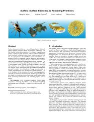
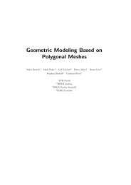
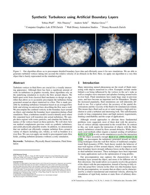
Synthetic Turbulence using Artificial Boundary LayersTobias Pfaff 1 Nils Thuerey 1 Andrew Selle 2 Markus Gross 1,31 Computer Graphics Lab, ETH Zurich 2 Walt Disney Animation Studios 3 Disney Research ZurichFigure 1: Our algorithm allows us to precompute detailed boundary layer data and efficiently reuse it for new simulations. We are able togenerates turbulent vortices taking into account the relative velocity of an obstacle in the flow. Here, we apply our algorithm to a very thinobject that is barely represented on the simulation grid.AbstractTurbulent vortices in fluid flows are crucial for a visually interestingappearance. Although there has been a significant amount ofwork on turbulence in graphics recently, these algorithms rely onthe underlying simulation to resolve the flow around objects. Webuild upon work from classical fluid mechanics to design an algorithmthat allows us to accurately precompute the turbulence beinggenerated around an object immersed in a flow. This is made possibleby modeling turbulence formation based on an averaged flowfield, and relying on universal laws describing the flow near a wall.We precompute the confined vorticity in the boundary layer aroundan object, and simulate the boundary layer separation during a fluidsimulation. Then, a turbulence model is used to identify areas wherethis separated layer will transition into actual turbulence. We samplethese regions with vortex particles, and simulate the further dynamicsof the vortices based on these particles. We will show howour method complements previous work on synthetic turbulence,and yields physically plausible results. In addition, we demonstratethat our method can efficiently compute turbulent flows around avariety of objects including cars, whisks, as well as boulders in ariver flow. We can even apply our model to precomputed static flowfields, yielding turbulent dynamics without a costly simulation.Keywords: Turbulence, Physically Based Animation, Fluid SimulationACM Reference FormatPfaff, T., Thuerey, N., Selle, A., Gross, M. 2009. Synthetic Turbulence using Artifi cial Boundary Layers.ACM Trans. Graph. 28, 5, Article 121 (December 2009), 10 pages. DOI = 10.1145/1618452.1618467http://doi.acm.org/10.1145/1618452.1618467.Copyright NoticePermission to make digital or hard copies of part or all of this work for personal or classroom use is grantedwithout fee provided that copies are not made or distributed for profi t or direct commercial advantageand that copies show this notice on the fi rst page or initial screen of a display along with the full citation.Copyrights for components of this work owned by others than ACM must be honored. Abstracting withcredit is permitted. To copy otherwise, to republish, to post on servers, to redistribute to lists, or to use anycomponent of this work in other works requires prior specifi c permission and/or a fee. Permissions may berequested from Publications Dept., ACM, Inc., 2 Penn Plaza, Suite 701, New York, NY 10121-0701, fax +1(212) 869-0481, or permissions@acm.org.© 2009 ACM 0730-0301/2009/05-ART121 $10.00 DOI 10.1145/1618452.1618467http://doi.acm.org/10.1145/1618452.16184671 IntroductionMany interesting natural phenomena are the result of fluids interactingwith objects immersed in a flow. Examples include smokebehind a car being influenced by the vortices in the car’s wake aswell as complex wave structures and splashes forming around rocksin river beds. Fluid simulations have made huge steps in previousyears, and have become an important tool for filmmakers. Despitethe increased popularity, fluid simulations are still inherently difficultto use. For a typical solver, the accuracy of the spatial discretizationsand the viscosity of the fluid to be simulated are related.This means that a fluid such as air or water requires a high grid resolutionto yield a turbulent and interesting look. This unfortunatelyresults in long computation times and high memory requirements,limiting controllability and the scope of applications.Although several approaches to alleviate these fundamentalproblems were suggested, most of them deal with the preservationof vortices already represented in the overall flow. In contrastto this, our work targets the interaction of objects with the fluid,namely turbulence created by flows around obstacles. While previouslyused methods either require a manual seeding of turbulence[Selle et al. 2005] or rely on the simulation to resolve the interactionwith the object accurately enough [Kim et al. 2008b; Narain et al.2008], we precompute the turbulence generated around an objectusing techniques from the wall flow theory of traditional computationalfluid dynamics (CFD). Such theory models the behavior ofnear-wall regions of flow around objects, which is important sincethese boundary layers strongly influence forces on the object as wellas shed turbulent structures. These techniques have been importantfor many applications such as the optimization of wing profiles.Our precomputation step captures the characteristics of theboundary layer around the object, and stores it for different sets offlow directions. Our model allows us to purely resolve the geometryof the object with the precomputation, instead of having to fully resolvethe actual flow velocity in the often very thin boundary layer.For the precomputation, we assume that an object can be characterizedby a relative translational and rotational velocity, allowing forsimulations of rigid body motion or static flows of arbitrary direction.ACM Transactions on Graphics, Vol. 28, No. 5, Article 121, Publication date: December 2009.

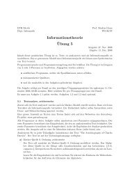
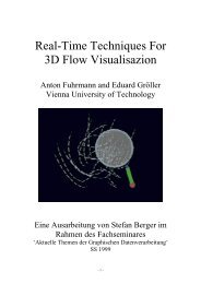
121:2 • T. Pfaff et al.1) Pre-compute ArtificialBoundary Layers2) Compute Flow Field 3) Re-use Boundary Layerand Compute Separation4) Identify TurbulentTransition Regions5) Simulate VortexDynamicsFigure 2: An overview of different steps of our algorithm. After precomputing the artificial boundary layer (1), we run a new simulation (2)and apply the confined vorticity from the precomputation (3). Regions transitioning into turbulence are identified with an approximation ofthe Reynolds stress (4). This results in the creation of vortex particles. Their dynamics are computed in an additional step (5).In a second step, we re-use our precomputed boundary layerdata to efficiently calculate where vortices are created around theobject in a separate simulation. We compute the evolution of vorticityaround the object, and estimate regions where this vorticitybecomes unstable to form actual turbulent vortices. In contrast totraditional CFD applications, we are not targeting averaged properties,such as the mean pressure distribution around an object. Ourgoal is to compute a visually interesting temporal evolution of theturbulence around the object. We achieve this by modeling the vorticeswith an improved variant of vortex particles [Selle et al. 2005].We create vortex particles based on boundary layer vorticity andsimulate their dynamics (as well as splitting and merging) based onturbulent energy transport and the vorticity equations of flow. Theresulting vorticity can even be reconstructed into a grid with higherresolution than the base simulation.Overall, our approach allows us to efficiently compute complexturbulent flows around objects without having to manually seed particlesor having to simulate on very high grid resolutions. Movingthe computations for the generation of turbulence into a preprocessingstep allows us to quickly set up new simulations around a givenobject. The contributions of our method are:• A new method to accurately track and precompute boundarylayer vorticity using an artificial boundary layer whose accuracyis independent of a final simulation resolution.• An algorithm to process the precomputed data in a dynamicsimulation to spawn vortices according to the current flow.• A vortex particle method that models vortex interactions andadheres to turbulent energy transport theory.Our method also elegantly handles turbulent free surface flows, atopic that has been barely studied in previous work other than thework of Selle et al. [2005] and Narain et al. [2008]. In addition, ourmethod can accurately compute turbulent wakes around objects thatare too fine to be resolved on the simulation grid. This is due to thefact that we decouple the resolution, and thus accuracy, of computationsfor the turbulence around obstacles, the actual simulation andthe evaluation of the vortex particles. Because our method separatesresolving the boundary layer and the actual flow, it can be seen asan example of the increasingly important paradigm of multi-scalephysics.Overview Our simulation method consists of a standard, gridbasedfluid solver, e.g. according to Stam [1999], augmented witha turbulence representation. We use an enhanced version of vortexparticles [Selle et al. 2005], which enforce a rotation in theflow around the particle’s position, to represent turbulence. The keypoint of our paper is an intelligent method to seed these particles.In § 3, we will develop a theory for this. In § 4, the dynamics of thevortex particles are described, and the coupling of the vortex particlesto the flow field is explained. The actual simulation loop andimplementation details are discussed in § 5.2 Related WorkStam [1999] popularized the unconditionally stable combination ofsemi-Lagrangian advection with first order pressure projection, butnumerical dissipation still plagued simulations. A common way tocombat dissipation is to attempt to more closely converge to thesolution. Adaptive grid methods [Losasso et al. 2004], [Feldmanet al. 2005], [Irving et al. 2006] address numerical dissipation withrefinement. However, this assumes only a small part of a simulationneeds high detail. One can also apply higher order advectionmethods such as Back and Forth Error Compensation and Correction[Kim et al. 2005], semi-Lagrangian MacCormack [Selle et al.2008], QUICK [Molemaker et al. 2008], or CIP methods (see e.g.[Kim et al. 2008a]). Alternatively, Fedkiw et al. [2001] advocatedetecting and amplifying existing vortices to combat dissipation.Mullen et al. [2009], on the other hand, propose an implicit energypreserving velocity integration scheme to solve the vorticity equation.Although precomputations are difficult for fluid simulations,Wicke et al. [Wicke et al. 2009] presented a method to precomputeand couple reduced bases of flows. These algorithms, however, stillrely on the underlying simulation to resolve the boundary layersaround objects.Many researchers have augmented or replaced basic fluid simulationwith synthetic turbulence. Stam [1993] introduced a methodthat used a Kolmogorov spectrum to produce procedural divergencefree turbulence. This approach was used to model nuclear explosionsand flames [Rasmussen et al. 2003; Lamorlette and Foster2002]. Bridson et al. [2007] suggest taking the curl of vector noisefields to produce divergence free velocity fields. They explicitly addresscomputing flows around objects efficiently by modulating thepotential field, however, their method does not model the complexturbulent effects near the wall. Most recently, researchers have consideredtransporting quantities with a lower resolution simulationwhich is used to generate detail [Kim et al. 2008b; Schechter andBridson 2008; Narain et al. 2008]. However, the treatment of obstaclesis not the focus of these techniques. Kim et al. [2008b] onlyextrapolate energies into obstacles to prevent artifacts and Narain etal. [2008] state that their approximation is not valid in the vicinityof obstacles.While the preceding approaches achieve interesting turbulent behaviorin fluid volumes, a major source of turbulence is interactionof fluids with solids. Two-way coupling of fluids has been addressedby Carlson et al. [2004], Guendelmann et al. [2003] andKlingner [2006]. More recently researchers have modeled subgridACM Transactions on Graphics, Vol. 28, No. 5, Article 121, Publication date: December 2009.

Synthetic Turbulence using Artificial Boundary Layers • 121:3interactions with objects more accurately through the use of apertures[Batty et al. 2007; Robinson-Mosher et al. 2008]. Nevertheless,very little previous work in graphics addresses the problem thatthe thin turbulent boundary layer is not resolved in the simulation,resulting in turbulence not being shed.3 Wall-Induced TurbulenceWhile turbulence in flows is generated by various processes, themost common and visually important one is turbulence generationat the flow boundaries. Therefore, our algorithms explicitly modelthis important process. Our method is based on wall flow theoryand turbulence modeling, which we will outline in § 3.1. A morethorough review can be found in the book by Pope [2000].3.1 Generation of turbulenceIn wall-bounded flows, wall friction enforces a tangential flow velocityof zero at the wall. This leads to the formation of a thin layerwith reduced flow speed, called the boundary layer. Fig. 3 shows avelocity profile in the boundary layer. It has been shown that thisprofile is equivalent for all wall-bound flows when using normalizedunits. This universal law of the wall was stated by van Driestin [1956].The gradient of tangential flow velocity in the boundary layerleads to the creation of a thin sheet of vorticity ω = ∇ × u. Forplanar walls, this vorticity remains mostly confined to the boundarylayer, and we will thus refer to it as confined vorticity. At regionsof high flow instability however, vorticity may be ejected from theboundary layer and enter the flow as turbulence. This happens e.g.at sharp edges, where the boundary layer is separated from the wall,and likely to become unstable, or when other turbulent structuresdisturb the boundary layer. This process of turbulence formation isreferred to as roll-up, and is the predominant mechanism of wallinducedturbulence generation [Jiménez and Orland 1993]. Thereis no theory quantitatively describing the boundary layer roll-upprocess. We will therefore model this process in a statistical sense,as explained below.Turbulence modeling We base our approach on CFD turbulencemodeling techniques. These techniques model statisticalproperties of turbulence based on the ensemble-average of the flowfield u. For a quasi-static flow, ergodicy permits us to use the timeaveragedflow field, i.e. the flow field with all fluctuating turbulentstructures averaged out, instead of the more complicated ensembleaveraging.One of the most important quantities that can be modeled in sucha way is the Reynolds stress tensor. It governs the transfer of energyfrom the bulk flow to turbulent structures, and thus the generationof turbulence. This fact is commonly used for ReynoldsaveragedNavier-Stokes simulations (RANS) or Large-Eddy Simulations(LES), and we will make use of it for our method as well.Next, we will describe how we model the boundary layer.Boundary layer modeling In order to accurately model wallinducedturbulence formation, we need to track the confined vorticity,simulate the boundary layer separation and finally identify thetransition points to turbulence.As the boundary layer, attached to an obstacle is very thin(smaller than simulation grid resolution in most cases), it is difficultto directly measure confined vorticity. Instead, we leverage the universallaw of the wall, and note that the confined vorticity only dependson the velocity scale and materials constants. For each pointin the wall-attached boundary layer we therefore determine the confinedvorticity asω ABL = β(U s × n) . (1)distance to wallviscoussublayerbufferlayerlog-lawregionThe velocity scale U s is the tangential component of the averagedflow velocity just outside the boundary layer. The constant β actangentialflow velocityFigure 3: The mean velocity profile near a wall (in normalizedunits) has the form shown above. This has been confirmed in numerousexperiments, and was formulated as a universal law by vanDriest.counts for the two material constants, skin friction coefficient andthe fluid viscosity. In our model, β is a user-defined parameter. Wecall the resulting field ω ABL the artificial boundary layer.On the other hand, boundary layer separation is an advectivetransport process. If the wall-attached part of the artificial boundarylayer is known, then the separation plume can be derived byadvecting this field with the flow field during the simulation run.The last missing part is to identify regions where the separatedboundary layer becomes unstable, and the confined vorticity ω ABLtransitions to free turbulence. The anisotropic part of the Reynoldstensor a i j , which is responsible for the production of turbulence, isa good indicator for such transition regions. We therefore define atransition probability density p T , which is used to seed turbulence,p T = c P ∆t ‖a i j‖|U 0 | 2 (2)such that regions with high Reynolds stresses are likely transitionregions. Here, ‖ · ‖ denotes the Euclidean matrix norm. Reynoldsstresses are normalized to a uniform scale by the inflow velocityU 0 , and c P is a parameter to control the seeding granularity. If usingvarying time-steps, p T has to be multiplied by ∆t to ensure consistentbehavior. In the following, we will describe how to computethe Reynolds stress tensor based on stresses in the averaged flowfield.Reynolds models The anisotropic component a i j of theReynolds stress tensor R i j can be expressed using the turbulent viscosityhypothesisa i j = −2ν T S i j , (3)where ν T is the turbulent viscosity and S i j denotes the strain tensorS i j = 1 ( ∂Ui+ ∂U )j. (4)2 ∂x j ∂x iThe turbulent viscosity can be expressed in terms of a so calledmixing length l m , which in near-wall regions is given by the distanceto the wall. We chose the model of Baldwin [1978] for modeling theturbulent viscosity:ν T ≈ l m 2 ‖Ω i j ‖ . (5)Here, Ω i j is the rotation tensor that can be computed asΩ i j = 1 ( ∂Ui− ∂U )j. (6)2 ∂x j ∂x iUsing these standard methods, it is possible to model the generationof turbulence using only the non-turbulent mean flow velocities.ACM Transactions on Graphics, Vol. 28, No. 5, Article 121, Publication date: December 2009.

Synthetic Turbulence using Artificial Boundary Layers • 121:5for describing dynamics, the injection and dissipation of energy viaparticle creation and dissipation is easier in an energy formulation.We will use a combination of both representations to leverage thestrengths of both models.Motion equation The dynamics of vorticity represented are describedby the vorticity formulation of the Navier-Stokes equation∂ ω∂t+ (u · ∇)ω = (ω · ∇)u + µ∇ 2 ω + ∇ × f , (9)where f denotes the external forces, and µ is the viscosity coefficient.The left side of the equation is inherently handled by advectingthe particles in the flow field of the Navier-Stokes solver.The first term on the right-hand side is the vortex stretching term. Itis computed by trilinear interpolation of the discrete gradient of thevelocity grid, and is used to adjust the particles’ vorticity magnitudeby ∆t(ω · ∇)u. This term is problematic as it might introduce exponentialaccumulation of vorticity magnitude in a particle. Therefore,the particle is rescaled after the update to preserve the magnitude,effectively only spinning the particle, but not altering its strength.The energy gain and loss is handled explicitly by energy dynamics,explained below. Similarly, the viscous diffusion term (the secondterm on the right hand side of Eq. (9)), will be handled by energydynamics, as it is not well represented by a vorticity exchangeamong sparsely sampled particles.The last term of Eq. (9) is handled with an underlying simulation,as external forces such as gravity are well-represented by aNavier-Stokes solver, and act on the vortex particles via the velocitygrid. This gives us a reduced formulation of Eq. (9) that conservesvorticity as well as energy. It is therefore orthogonal to the energytransfer, the computation of which we will describe next.Energy dynamics The dynamics of the turbulent kinetic energyE are covered by the energy transport equation [Pope 2000]∂E∂t+ (u · ∇)E = −∇ · T + P − ε (10)The left hand side again is handled by advection of the particles.The right-hand side consists of production P, dissipation ε and theenergy transfer term ∇ · T. These quantities are in general complexto model, especially in the model-dependent range. For the productionterm, we can use the information from our artificial boundarylayer (see § 3.2). The dissipation ε occurs at wavenumbers thatare usually well below the resolved grid resolutions. Dissipation istherefore implemented by removing particles whose radii are toosmall to be represented on the grid. We use a threshold of 2∆x forour simulations. Finally, for handling the remaining energy transferterm for T of Eq. (10), we distinguish the following two cases:1. The particle is in the inertial subrange. We represent the energycascade by decaying a particle with wavenumber κ a inton particles of smaller wavenumber κ b . We typically use n=2in our simulations. From Kolmogorov’s law, we can derivea timescale of decay as ∆t = C(κ − 2 3a − κ − 2 3b ), where C denotesa parameter that depends on the rate of dissipation ε.In practice we can use a value normalized by the averagedflow U here. We also know that for the turbulent energiesE a /E b = n(κ a /κ b ) − 5 3 holds, which is used to derive the vorticitymagnitude of the new particles. For practical reasons,we also add a small position and angle displacement to thenew vortex particles, as they would otherwise lump together.2. The particle is in the model-dependent range. As transfer cannotbe easily described in this regime, a simple heuristic isused. Typically, small vortices with aligned direction tend toform larger vortices in this range. Therefore, we merge vortexparticles in the model-dependent range with a distance of lessthan the particle radius to a single larger vortex particle. Here,the vortex magnitude is chosen so that total the energy is conservedas E new = E 1 + E 2 . As very small and strong vortexparticles might induce stability problems, we also conservethe energy density, i.e. E newV new= E 1V 1+ E 2V 2. This specifies the radiusand strength of the merged particle. The new direction isobtained by a weighted average, with the respective energiesas a weight.4.3 Vorticity SynthesisTurbulence synthesis is performed by enforcing the vortex particles’vorticity on the simulation velocity grid. Each vortex particlehas a vorticity vector ω P , encoding magnitude and rotation axis,and a kernel over which this value is applied.Kernel For the direct regulation of vorticity, a kernel with thefollowing properties is desired: at the vortex particle center, vorticityshould be equal to ω P . Also, the resulting vector field shouldmainly contain rotation around ω P , and smoothly fade out with theparticle radius without causing discontinuities. And lastly, the associatedvelocity field, and its integral, which is needed for e.g. energycalculation, should be a simple analytic form. We chose a Gaussianpeak with standard deviation of σ in the vector potential to meetthese requirements. In cylindrical coordinates, it is given byΨ(z,ϕ,ρ) = −|ω P |σ 2 exp −ρ2 −z 22σ 2 e z , (11)where the vortex axis e z is aligned with ω P . We can then derive thevelocity fieldand the vorticity kernelu = ∇ × Ψ = −|ω P |ρ exp −ρ2 −z 22σ 2 e ϕ , (12)ω = ∇ × u = − |ω P |σ 2 (ρze ϕ − (ρ 2 − 2σ 2 )e z)exp −ρ2 −z 22σ 2 . (13)A cut-off radius is used to make the kernel support finite. We user = √ 6σ at which point the exponential term of the kernel functionhas fallen to 10 −3 . The length scale is defined at the kernels’ origin,so that its wavenumber is κ = σ 1 . For the contained energy E ∝ω 2 P σ 5 holds.Kernel Evaluation This is a three-step process: First, the vorticityfield ω = ∇ × u of the velocity grid is computed by finitedifferences. Second, all particle vorticity kernels are summed up toobtain a desired vorticity field ω D . And third, each particle adds itskernel to the velocity field, scaled by a weight w k , computed as:w k = ∑ kernel(ω D − ω) · ¯ω P∑ kernel ω D · ¯ω P, (14)where ¯ω P is the particles’ normalized rotation axis. The dot productwith ¯ω P ensures that only the vortex particles’ direction is considered,and the kernel is normalized by the sum of desired vorticity.We achieve an exact regulation of the vorticity sum under the kernelin one timestep by this process.Vortex particle seeding As explained in 3.2, particles will beseeded in regions of high normalized Reynolds stress. Based on theprobability p T (x) from Eq. (8), a particle is created at position x.All confined vorticity ω ABL within the particle’s radius is removedfrom the artificial boundary layer, and the particle’s strength anddirection ω P are set such that the vorticity integrated over the kernelACM Transactions on Graphics, Vol. 28, No. 5, Article 121, Publication date: December 2009.

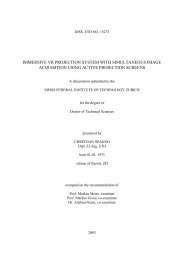
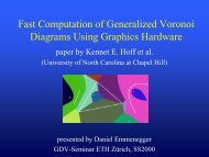
121:6 • T. Pfaff et al.Figure 6: Example of a moving object inducing turbulence in its wake. The top row of images shows a simulation without vortex particles,the bottom row was simulated using our method.equals the removed vorticity sum. We choose the particle radius tobe as large as possible without touching an object. We allow forradii up to a size r max which is fully resolved by the main simulation(we have used a value of r max = 6∆x below).The constant c P in Eq. (8) controls the granularity of the seedingprocess. If set to a high value, confined vorticity is turned intofree turbulence relatively quickly. This results in a large number ofweaker particles near the object, which then merge to large vortices.On the other hand, if c P is set to a high value, the artificial boundarylayer plume can grow, and fewer, stronger particles form. Withan appropriately chosen c P , numerical cost can be kept low whileavoiding popping artifacts that may occur if overly large particlesare seeded. We use a c p of ≈ 1 − 4 in our simulations.5 Implementation5.1 PrecomputationFor precomputing the artificial boundary layer, it is essential to resolvethe mean flow around an object. This can be done using timeaveragingover a long period of time with a standard solver, or usinga RANS solver. As we are only interested in the velocities aroundthe boundary layer, we have used a standard solver with an artificiallyincreased viscosity in the form of a diffusion step for thevelocities. Due to the increased viscous effect, it stabilizes quicklyand an average over fewer frames can be used. We have found thatusing the more complex RANS or longtime-averaging does not payoff visually compared to this more efficient solution. After obtainingthe averaged flow field, the boundary layer is calculated accordingto the pseudo-code (Fig. 5) and stored as a point set.Moving objects To precompute the flow for scenes with movingobjects, the boundary layer around each moving objects is precalculated.If the object can move and rotate freely, or its movementis not known a priori, our algorithm allows us to precompute thewhole range of movement directions to later on generate arbitrarysimulations of the object in a flow. For this, we split the movementinto a translational and a rotational component and precompute artificialboundary layers for each.To perform the precomputation, the object is placed in the centerof a simulation grid. The domain box is chosen large enough notto disturb the flow around the object. For the translational component,we leave the object fixed and use different inflow velocities,defined as boundary conditions on the domain box. As ω ABL is linearin the velocity magnitude, we only need to sample the velocitydirection. In our simulations, we use 10 × 20 samples in sphericalcoordinates. For the rotational component, the object is placed ina standing fluid, and we rotate the object with normalized speedaround a chosen axis. Again, we use 10 × 20 samples in sphericalcoordinates to sample the rotation axis direction.Figure 7: The top picture show a basic simulation of a fluid flowingleft to right over a cavity. This flow produces a big vortex in thecavity, but is unable to capture any generation of turbulence fromthe walls. With our method (at the bottom) we are able to identifythe confined vorticity shedding off the two edges of the cavity, andintroduce corresponding vortex particles to represent the turbulentstructures forming in the flow.The simulations stabilize quickly due to the increased viscosity.We have used 50 steps for the examples shown in our video. In theprecomputations for the rotational component, this is equivalent toone full rotation. After stabilizing, we average the velocities overanother 50 frames. We note that precomputations for each directioncan be trivially done in parallel.Applying the precomputed set At simulation time, we determinethe objects linear velocity relative to the scene, and its rotationaxis. We then look up the nearest values in the precomputeddatabase. A bilinear spherical interpolation is performed for boththe linear velocity direction as well as the rotation axis. The resultsof the interpolation are scaled by respective magnitude and added.We have performed error measurements for the linear interpolationof the boundary layer values. The corresponding graph can be seenin Fig. 12. Our choice of 20 directional samples in the azimuthmeans we have an interpolation error of 1.6%. As the decompositioninto rotational and linear component is only an approximation,we have also measured its error for the car model (Fig. 6). In thisACM Transactions on Graphics, Vol. 28, No. 5, Article 121, Publication date: December 2009.

Synthetic Turbulence using Artificial Boundary Layers • 121:7Figure 8: Comparison between a reference simulation (top picture),a simulation with randomly seeded vortex particles along the walls(middle), and our method (bottom). The random vortex particles destroythe overall flow structure, although the number and strengthof the vortex particles are similar to those used in our method. Ourapproach correctly identifies the turbulence being shed off the step,similar to the reference simulation at the top, and introduces particleswith a correct orientation locally into the flow.case the error is 8% on average, and thus small enough not to causevisual artifacts.It is not necessary to fully resolve the boundary layer during theprecomputations, as our model described in § 3.1 takes care of this.Instead, one should make sure the resolution of the precomputationis sufficiently fine to resolve all important geometric features ofthe object. This is eased by the precomputation focusing only onthat object, even if it will only occupy a tiny fraction of the finalsimulation domain. In addition, since the precomputation can beused on many simulations, a high resolution precomputation gridcan quickly pay off. In § 6 we demonstrate the effectiveness of theprecomputation even when an object is extremely thin.5.2 Simulation loopFor the actual simulation, a standard fluid solver and a vortex particlesystem are coupled. In each simulation step, the artificial boundarylayer is updated, new vortex particles are created and vortexparticle dynamics are applied. Afterwards, the turbulence forces areadded to the flow field, and finally, the remaining steps of the standardfluid simulation are performed. This is repeated each timestep.Pseudo-code for this extended simulation loop can be foundin Fig. 9Note that we can also independently choose a higher grid resolutionfor the evaluation of the vortex particles. This allows us to moreaccurately evaluate the particle kernels, which is especially usefulfor small scale vortex details. This high resolution velocity field isdown-sampled for the main simulation steps (line 28 in the pseudocode),and up-sampled for our algorithm before starting with line 1.Performing the algorithm (line 1–25) with a higher resolution enablesus to simulate detailed features, e.g., when advecting smokedensities or a free surface level set, while the costly pressure projectionoperates on a small grid resolution. Typically, we have useda two times higher resolution for the examples below.1: // Initialize boundary layer2: for each voxel x on an obstacle boundary do3: Find corresponding (x pre , ω pre ) in precomputed set4: // Initialize wall-attached ABL5: ω ABL (x) ← max(ω ABL (x), ω pre )6: end for7:8: // Simulate boundary layer seperation9: Advect ω ABL with the main flow10:11: // Seed vortex particles12: for each voxel x with ω ABL (x) ≠ 0 do13: p T ← 2c P ∆t (l m |ω ABL (x)|/|U 0 |) 214: if random() < p T then15: (Y ) ← voxels within particle radius of x16: ω S = ∑ (Y ) ω ABL // sum within particle radius17: ω ABL (Y ) ← 0 // remove vorticity from ABL18: Seed particle at x with total vorticity ω S19: end if20: end for21:22: // Vortex particle dynamics23: Advect vortex particles24: Merge, split, dissipate vortex particles (§ 4.2)25: Synthesize turbulence (§ 4.3)26:27: // Standard fluid simulation steps28: Velocity self-advection, pressure projection etc.Figure 9: Pseudo-code for a main simulation loop including ourturbulence model.6 Results and DiscussionIn the following section we discuss comparisons of our method toprevious work and a reference simulation. In addition, we demonstrateseveral complex examples of turbulence being generatedaround moving objects or due to effects such as wind or a flowingriver.Comparisons In Fig. 7 the effect of our wall-induced turbulencecan be seen for the flow over a cavity with a grid resolution of120 × 60 × 40. The top image shows a standard, unmodified simulation,while the lower image uses our algorithm to introduce wallinducedturbulence. Both simulations use the same grid resolution,but the unmodified simulation is unable to capture any turbulencebeing generated from the shearing near the walls. Our simulationexhibits complex vortices due to the vorticity generated at the wallboundaries. To compare our method to approaches for synthetic detailgeneration, we have simulated the same cavity setup includingwavelet turbulence, using the implementation available on thepaper’s website [Kim et al. 2008b]. Wavelet turbulence successfullyadds small detail to the overall flow, but has difficulties introducinglarger vortices to the strong horizontal motion. In contrast,our method introduces persistent larger vortices, while the resultingsmoke filaments are successfully broken up by the wavelet turbulence.This shows that our method is suitable for bridging the gapbetween small synthetic vortices and the vortices resolved by a standardsimulation.We use the setup shown in Fig. 8 to compare our method withnormal vortex particles [Selle et al. 2005]. The simulations nowfocus on the left edge of the cavity. The top image shows a referencesimulation, using a four times increased grid resolution. Notethat the flow along the wall to the left is completely straight, whileturbulent structures form to the right of the backward facing step.This behavior has been confirmed in various experiments and sim-ACM Transactions on Graphics, Vol. 28, No. 5, Article 121, Publication date: December 2009.

121:8 • T. Pfaff et al.confinement uniformly amplified vorticity magnitude. Our method,like vortex particles, overcomes this by allowing local modelingof vorticity, including effects like tilting and stretching. However,by modeling the boundary layer and considering the directions ofparticles vortices with Eq. (1), we are able to keep vortex particlesfrom disturbing the bulk flow. This allows us to use vortex particlesof larger magnitude than the randomly seeded vortex particles.Complex Examples Next we consider examples with more complexgeometry. Fig. 6 shows the simulation of a moving car that isemitting smoke. It can be observed how our model reproduces thedependence of turbulence strength from the cars velocity. As canbe seen in the top row of Fig. 6, a normal simulation of the sameresolution would not resolve any shed vortices at the car’s surface.Second, Fig. 1 shows a thin whisk geometry stirring smoke. Theboundary layer precomputation was done with a high resolutiongrid that resolved the whisk’s wires, while its subsequent use ina smoke simulation was done on a much coarser grid. The standardgrid did not resolve the wires, and only approximate velocityboundary conditions were set, resulting in the fluid slightly followingthe whisk’s motion. Still, our algorithm was able to accuratelygenerate vortices that are produced by its motion.In Fig. 11 we show how our method works in conjunction withstatic flow fields. In this case we precompute a snapshot imageof static flow around the object, and use it to advect the boundarylayer, the vortex particles and the smoke densities. This simpleform of simulation works without an expensive pressure correctionstep. Despite the simple underlying setup, we are able to producecomplex structures forming in the wake behind the obstacle fromthe interactions of the vortex particles amongst themselves. Lastly,we demonstrate that our method can be easily extended to free surfacesin Fig. 10. Here three obstacles in the liquid produce turbulentwakes behind them. For this simulation, a particle level set [Enrightet al. 2002] was used to represent the liquid’s surface. Similarto particles near obstacle walls, we reduce a particle’s kernel sizeonce it extends past the liquid phase to avoid non-divergence freevelocity fields.Detailed grid sizes and timings for the examples above can befound in Table 1. The performance was measured on an Intel Corei7 CPU with 3.0 GHz. The majority of the time used for our approach(denoted by ABL time in Table 1) is taken up by the advectionof the artificial boundary layer. For the liquid example ofFig. 10, the performance is strongly dominated by the particle levelset. Overall, we achieve computing times ranging from 10 to 20seconds per frame on average. An exception is the example with astatic flow field, which requires only 1.3 seconds per frame.Figure 10: Our algorithm naturally extends to simulations of liquids.Here, we apply our algorithm to a river flow around three obstacles,resulting in turbulent wakes behind them.ulations (e.g. [Le et al. 1997]). The middle image shows the flowafter randomly introducing vortex particles along the walls. Naturally,the vortex particles do not take the overall flow into account,and strongly distort the structure of the flow. Our method, shownin the bottom picture, is able to recover the vortices being shed offthe step, without distorting the flow along the wall to the left. Althoughwe are not able to fully recover the flow of the referencesimulation due to the different numerical viscosities, our method isable to qualitatively capture the wall-induced turbulence at a muchlower computational cost. On average, the time per frame for thereference simulation was 218 times higher than for the simulationwith our algorithm.The limitation that motivated vortex particles was that vorticityLimitations A limitation of our method is that our precomputationcurrently assumes a rigid object, making it difficult to apply itto deforming objects such as cloth. To resolve this, a RANS solvercould be coupled to a normal fluid solver to determine the currentshear stresses at the object surface. Alternatively, it may be possibleto precompute suitable boundary layer data for deforming objectsby making use of data compression schemes. Also, our approach forthe precomputation assumes the flow around the object can be describedby the translational and rotational velocity components. Ifthe flow around the object varies strongly, e.g., due to strong externalforces or due to multiple objects in close vicinity, the resultingconfined vorticity can differ from the desired values .Extending our approach to handle this more accurately is interestingfuture work. In addition, a trade-off of our method is theuse of vorticity reconstruction at a higher resolution. While this allowsus to go beyond the coarse simulation Nyquist limit and gethigher resolution detail (a limitation of the original vortex particlemethod), it means the domain and object boundaries as well as thefree-surface boundary conditions are not as well modeled by thereconstructed high resolution velocity field.ACM Transactions on Graphics, Vol. 28, No. 5, Article 121, Publication date: December 2009.

121:10 • T. Pfaff et al.FELDMAN, B. E., O’BRIEN, J. F., AND KLINGNER, B. M. 2005.Animating gases with hybrid meshes. In Proceedings of ACMSIGGRAPH.GUENDELMAN, E., BRIDSON, R., AND FEDKIW, R. 2003. Nonconvexrigid bodies with stacking. ACM Trans. Graph. (SIG-GRAPH Proc.) 22, 3, 871–878.IRVING, G., GUENDELMAN, E., LOSASSO, F., AND FEDKIW, R.2006. Efficient simulation of large bodies of water by couplingtwo and three dimensional techniques. ACM Trans. Graph. (SIG-GRAPH Proc.) 25, 3, 805–811.JIMÉNEZ, J., AND ORLAND, P. 1993. The rollup of a vortex layernear a wall. Journal of Fluid Mechanics.KIM, B., LIU, Y., LLAMAS, I., AND ROSSIGNAC, J. 2005. Flowfixer:Using BFECC for fluid simulation. In Proceedings of EurographicsWorkshop on Natural Phenomena.KIM, D., YOUNG SONG, O., AND KO, H.-S. 2008. A semilagrangiancip fluid solver without dimensional splitting. Comput.Graph. Forum (Proc. Eurographics) 27, 2, 467–475.SCHECHTER, H., AND BRIDSON, R. 2008. Evolving sub-gridturbulence for smoke animation. In Proceedings of the 2008ACM/Eurographics Symposium on Computer Animation.SELLE, A., RASMUSSEN, N., AND FEDKIW, R. 2005. A vortexparticle method for smoke, water and explosions. In Proceedingsof SIGGRAPH.SELLE, A., FEDKIW, R., KIM, B., LIU, Y., AND ROSSIGNAC, J.2008. An unconditionally stable MacCormack method. Journalof Scientific Computing.STAM, J., AND FIUME, E. 1993. Turbulent wind fields for gaseousphenomena. In Proceedings of ACM SIGGRAPH.STAM, J. 1999. Stable fluids. In Proceedings of ACM SIGGRAPH.WICKE, M., STANTON, M., AND TREUILLE, A. 2009. ModularBases for Fluid Dynamics. ACM SIGGRAPH Papers 28 (Aug),Article 39.KIM, T., THUEREY, N., JAMES, D., AND GROSS, M. 2008.Wavelet Turbulence for Fluid Simulation. ACM SIGGRAPH Papers27, 3 (Aug), Article 6.KLINGNER, B. M., FELDMAN, B. E., CHENTANEZ, N., ANDO’BRIEN, J. F. 2006. Fluid animation with dynamic meshes. InProceedings of ACM SIGGRAPH.KOLMOGOROV, A. 1941. The local structure of turbulence in incompressibleviscous fluid for very large reynolds number. Dokl.Akad. Nauk SSSR 30.LAMORLETTE, A., AND FOSTER, N. 2002. Structural modelingof flames for a production environment. In Proceedings of ACMSIGGRAPH.LE, H., MOIN, P., AND KIM, J. 1997. Direct numerical simulationof turbulent flow over a backward-facing step. J. Fluid Mech.330, 01, 349–374.LOSASSO, F., GIBOU, F., AND FEDKIW, R. 2004. Simulatingwater and smoke with an octree data structure. Proceedings ofACM SIGGRAPH, 457–462.MOLEMAKER, J., COHEN, J. M., PATEL, S., AND NOH, J. 2008.Low viscosity flow simulations for animation. In ACM SIG-GRAPH / Eurographics Symp. on Comp. Anim., 9–18.MULLEN, P., CRANE, K., PAVLOV, D., TONG, Y., AND DES-BRUN, M. 2009. Energy-Preserving Integrators for Fluid Animation.ACM SIGGRAPH Papers 28, 3 (Aug).NARAIN, R., SEWALL, J., CARLSON, M., AND LIN, M. C. 2008.Fast animation of turbulence using energy transport and proceduralsynthesis. ACM SIGGRAPH Asia papers, Article 166.POPE, S. B. 2000. Turbulent Flows. Cambridge University Press.RASMUSSEN, N., NGUYEN, D. Q., GEIGER, W., AND FEDKIW,R. 2003. Smoke simulation for large scale phenomena. In Proceedingsof ACM SIGGRAPH.ROBINSON-MOSHER, A., SHINAR, T., GRETARSSON, J., SU, J.,AND FEDKIW, R. 2008. Two-way coupling of fluids to rigidand deformable solids and shells. ACM SIGGRAPH papers 27,3 (Aug.), Article 46.ACM Transactions on Graphics, Vol. 28, No. 5, Article 121, Publication date: December 2009.