Empirical Dual Energy Calibration (EDEC) for Cone-Beam ...

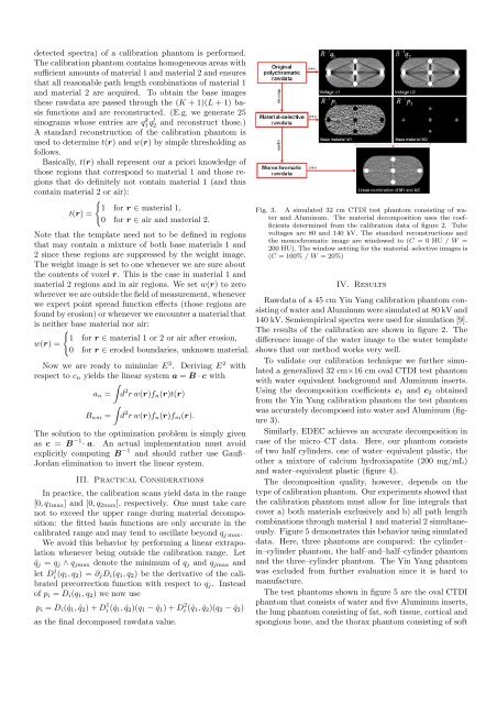
detected spectra) of a calibration phantom is performed.The calibration phantom contains homogeneous areas withsufficient amounts of material 1 and material 2 and ensuresthat all reasonable path length combinations of material 1and material 2 are acquired. To obtain the base imagesthese rawdata are passed through the (K + 1)(L + 1) basisfunctions and are reconstructed. (E.g. we generate 25sinograms whose entries are q1 kql 2 and reconstruct those.)A standard reconstruction of the calibration phantom isused to determine t(r) and w(r) by simple thresholding asfollows.Basically, t(r) shall represent our a priori knowledge ofthose regions that correspond to material 1 and those regionsthat do definitely not contain material 1 (and thuscontain material 2 or air):{1 for r ∈ material 1,t(r) =0 for r ∈ air and material 2.Note that the template need not to be defined in regionsthat may contain a mixture of both base materials 1 and2 since these regions are suppressed by the weight image.The weight image is set to one whenever we are sure aboutthe contents of voxel r. This is the case in material 1 andmaterial 2 regions and in air regions. We set w(r) to zerowherever we are outside the field of measurement, wheneverwe expect point spread function effects (those regions arefound by erosion) or whenever we encounter a material thatis neither base material nor air:{1 for r ∈ material 1 or 2 or air after erosion,w(r) =0 for r ∈ eroded boundaries, unknown material.Now we are ready to minimize E 2 . Deriving E 2 withrespect to c n yields the linear system a = B · c with∫a n = d 2 r w(r)f n (r)t(r)∫B nm = d 2 r w(r)f n (r)f m (r).The solution to the optimization problem is simply givenas c = B −1· a. An actual implementation must avoidexplicitly computing B −1 and should rather use Gauß–Jordan elimination to invert the linear system.III. Practical ConsiderationsIn practice, the calibration scans yield data in the range[0, q 1max ] and [0, q 2max ], respectively. One must take carenot to exceed the upper range during material decomposition:the fitted basis functions are only accurate in thecalibrated range and may tend to oscillate beyond q j max .We avoid this behavior by performing a linear extrapolationwhenever being outside the calibration range. Letˆq j = q j ∧ q jmax denote the minimum of q j and q jmax andlet D j i (q 1, q 2 ) = ∂ j D i (q 1 , q 2 ) be the derivative of the calibratedprecorrection function with respect to q j . Insteadof p i = D i (q 1 , q 2 ) we now usep i = D i (ˆq 1 , ˆq 2 ) + D 1 i (ˆq 1 , ˆq 2 )(q 1 − ˆq 1 ) + D 2 i (ˆq 1 , ˆq 2 )(q 2 − ˆq 2 )as the final decomposed rawdata value.Fig. 3. A simulated 32 cm CTDI test phantom consisting of waterand Aluminum. The material decomposition uses the coefficientsdetermined from the calibration data of figure 2. Tubevoltages are 80 and 140 kV. The standard reconstructions andthe monochromatic image are windowed to (C = 0 HU / W =200 HU). The window setting for the material–selective images is(C = 100% / W = 20%)IV. ResultsRawdata of a 45 cm Yin Yang calibration phantom consistingof water and Aluminum were simulated at 80 kV and140 kV. Semiempirical spectra were used for simulation [9].The results of the calibration are shown in figure 2. Thedifference image of the water image to the water templateshows that our method works very well.To validate our calibration technique we further simulateda generalized 32 cm×16 cm oval CTDI test phantomwith water equivalent background and Aluminum inserts.Using the decomposition coefficients c 1 and c 2 obtainedfrom the Yin Yang calibration phantom the test phantomwas accurately decomposed into water and Aluminum (figure3).Similarly, EDEC achieves an accurate decomposition incase of the micro–CT data. Here, our phantom consistsof two half cylinders, one of water–equivalent plastic, theother a mixture of calcium hydroxiapatite (200 mg/mL)and water–equivalent plastic (figure 4).The decomposition quality, however, depends on thetype of calibration phantom. Our experiments showed thatthe calibration phantom must allow for line integrals thatcover a) both materials exclusively and b) all path lengthcombinations through material 1 and material 2 simultaneously.Figure 5 demonstrates this behavior using simulateddata. Here, three phantoms are compared: the cylinder–in–cylinder phantom, the half–and–half–cylinder phantomand the three–cylinder phantom. The Yin Yang phantomwas excluded from further evaluation since it is hard tomanufacture.The test phantoms shown in figure 5 are the oval CTDIphantom that consists of water and five Aluminum inserts,the lung phantom consisting of fat, soft tissue, cortical andspongious bone, and the thorax phantom consisting of soft