Quantum Theory - Particle Physics Group

Chapter 1Introduction1.1 Historical notesIn the nineteenth century the profession of a specialized scientist was created and the mainscientific activity moved to university-like institutions. As a result scientific research flourished.One of the major and at the same time one of the oldest branches of physics was mechanics.Its foundation dates back to 1687, when Isaac Newton (1642–1727) formulated the principlesof mechanics and the gravitational law. The theory was further developed, among others, byJoseph Louis Lagrange (1736–1813), who formulated the dynamical equations, Carl FriedrichGauss (1777–1855), who introduced the ‘principle of least constraints’, as well as WilliamRowan Hamilton (1805–1865) and Carl Gustav Jacob Jacobi (1804–1851), who worked out anew scheme of mechanics. They stated that motions of objects in nature always occur withleast action, which was defined as the time integral over the so-called Lagrange function.On the basis of these discoveries thermodynamics was developed as a new branch of physics.Julius Robert Mayer (1814–1878) and James Prescott Joule (1818–1889) found out that heatfully corresponds to energy. The first and the second law of thermodynamics were first explicitlystated in a book by Rudolf Emanuel Clausius (1822–1888) in 1850. Clausius also shaped theconcept of entropy in 1865. Maxwell’s velocity distribution for the kinetic theory of gaseswas then explained by Boltzmann (1844–1906) with statistical mechanics. At the end of the19 th century this lead to the important problem of blackbody radiation, i.e. the quest for atheoretical understanding of the spectrum emitted by a perfect absorber (see chapter 1.2.1).Electrodynamics and optics were two separate disciplines until Heinrich Hertz (1857–1894)proved in 1888 that light possesses all characteristics of an electromagnetic wave. The firstquantitative description of an electrical force (attractive or repulsive) was made by CharlesAuguste de Coulomb (1736–1806) in 1785. André Marie Ampère (1775–1836) was the first tospeak of electrodynamics in 1822. In 1826 Georg Simon Ohm (1787–1854) formulated what is1

CHAPTER 1. INTRODUCTION 2nowadays known as Ohm’s law. In 1833 Gauss and Wilhelm Weber (1804–1891) invented thetelegraph. One of the most important contributions was made by Michael Faraday (1792–1867)who discovered electromagnetic induction and electrolysis. Based on this work James ClerkMaxwell (1831–1879) found a complete system of equations that describes all electromagneticphenomena.We conclude our excursion into the evolution of physics till the beginning of the 20 th centurywith a short glance at atomism. In ancient Greece, Demokritus introduced the idea of atomsas indivisible building block of matter. This idea was reintroduced in the 17 th century afterit had been mostly forgotten throughout the middle ages. Chemists focused on matter thatcould not be separated by chemical methods. Physicists, on the other hand, tried to explainphenomena such as pressure, temperature, specific heat and viscosity in terms of the particles(molecules) that gases consist of. This approach is called the kinetic theory of gases. Out ofthis statistical mechanics evolved. At the beginning of the 20 th century the atomic hypothesiswas at last widely accepted among the scientific community. It was not until 1905, however,that a theoretical proof for the existence of atoms was made simultaneously by Albert Einstein(1879–1955) and Marian Smoluchowski (1872–1917) in their work on Brownian motion. Stillthe structure of an atom and the ways in which the atoms of different elements differ were notyet understood at all. All in all, one can say that atomic physics was in its infancy at the turnof the century.In the late 19 th century some very important discoveries were made: In 1885 Wilhelm ConradRöntgen (1845–1923) discovered what he called X-rays. This phenomenon reminded Antoine-Henri Becquerel (1852-1908) of his work on phosphorescent stone and he began to search fora stone with similar properties. He finally found one – a uranium salt – and realized that hehad observed a new kind of radiation emitted by radioactive material. This radiation lateron turned out to be a very powerful tool for investigating atomic structure. In 1897 JosephJohn Thomson (1856–1940) was able to identify the first elementary particle, the electron,and to determine its charge to mass ratio. The reaction of the scientific world was ratherunenthusiastic. Some physicists didn’t even believe in the concept of atoms. Others thoughtthat atom and electrons were too small to be made objects of speculation. Later, Lord Kelvinand J.J. Thompson together developed a theory of atomic structure.The 20 th centuryThere were some physicists at the end of the 19 th century who believed that physics had cometo some kind of an “end of evolution” and that there was hardly anything interesting left tobe found out. Classical mechanics was able to describe almost all phenomena that had beendetected and thus seemed to be satisfactory. It was a simple and unified theory.

CHAPTER 1. INTRODUCTION 3Physicists distinguished two completely different categories of objects – matter and radiation:According to Newtonian mechanics matter is built out of localizable corpuscles with awell-defined position and velocity. One can thus compute the time evolution of a system assoon as one knows this data at a given moment. The corpuscular theory could even be extendedto the microscopic scale of solid bodies (i.e. to molecules or atoms). According to thermodynamicsand statistical mechanics macroscopic parameters thus derive from the motion of the(microscopic) particles. Radiation, on the other hand, could well be explained with Maxwell’slaws that are able to link electromagnetism, optics and acoustics. As light was capable of interferenceand diffraction, which are clearly associated with waves, light was eventually consideredto be a form of radiation.At the beginning of the 20 th century some experiments and theoretical problems implied,however, that this distinction between radiation and matter was not entirely valid. Physicistswere confronted with a bunch of data that seemed hard to explain within the framework ofwhat we now call classical physics and were even forced to look for different and at first strangenew concepts. This lead to the idea of quantization of physical entities and to wave-particledualism. The important achievements of quantum physics in the first three decades of the newcentury include the following:1900 Max Planck derives his formula for blackbody radiation by introducing a constant hthat determines the sizes of energy packages, called quanta, of electromagnetic radiation.1905 Albert Einstein explaines the photoelectric effect in terms of the same constant.1906 J.J. Thompson discovers the proton.1910 Robert Millikan measures the elementary electric charge.1911 After observations on the scattering of alpha particles caused by atoms, ErnestRutherford introduces the first modern picture of the atom.1913 Niels Bohr explains spectral lines and the stability of atoms by postulating quantizationof angular momentum.1923 Arthur Compton gives an explanation for the scattering of photons on electrons byassigning the momentum ⃗p = ⃗ k to photons.1924 Wolfgang Pauli formulates his exclusion principle.1925 Louis de Broglie’s doctoral thesis states that matter particles like photons areassociated to waves of wavelength λ = h/p.1925 Werner Heisenberg invents matrix mechanics, which assigns noncommuting matrixoperators to dynamical variables.

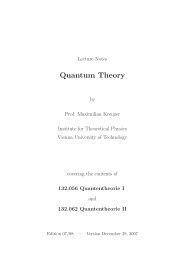
CHAPTER 1. INTRODUCTION 6This formula fits strikingly well to the experimentally obtained curves. It looks similar tothe Rayleigh-Jeans approximation, but the factor [e hνk BT − 1] −1 prevents the expression fromdiverging at higher frequencies (see figure 1.2).Figure 1.2: Comparison of the results for the spectrum of a blackbody according to Wien,Rayleigh-Jeans and PlanckAlthough Planck received a Nobel prize in 1918 for his ideas, his explanation of the spectrumof blackbody radiation did not take the world by storm at first. It seemed as if he hadconstructed a theory derived from experiment, but based on a hypothesis with no experimentalbasis.1.2.2 The photoelectric effectFive years later Einstein built on the ad hoc hypothesis of the quantization of energy to explainthe phenomenon of the photoelectric effect. This effect was first observed by Hertz in 1887: Ifan alkali metal is irradiated by light with a frequency larger than a certain minimum frequency(which depends on the metal) electrons are emitted by this metal. It is interesting that thevelocity of the electrons (and thus their energy) is only dependent on the frequency of the lightbeam hitting the metal, but not on its intensity. Classical physics is not able to explain theν–proportionality of this effect. Assuming light to be an electromagnetic wave, the electronsof the metal should absorb an energy that is increasing with the intensity of the light beamuntil their velocity is high enough to overcome the potential well. According to this, we shouldbe able to observe a delay between the start of the irradiation and the onset of the emissionof electrons. This delay has not been measured until today, even though by now we would beable to do so (if it existed). Classical physics thus fails to explain this effect correctly.Einstein took up the idea of Planck and even went a bit further. He assumed that lightconsisted of particles, called photons, with the energy hν. When one of these corpuscles encountersan electron of the metal, it is absorbed and the electron receives its energy hν (at oneinstant). If this energy is large enough for the electron to overcome the potential of the atom,

CHAPTER 1. INTRODUCTION 7it escapes. The energy of such an electron would be12 mv2 = hν − W, (1.5)where W is the work needed to free an electron from the potential well. This theory is incomplete accord with the experiment.At this time the whole extent of the idea of energy or light quanta could not yet be perceived.Planck thought that his hypothesis was a mere complement to the theories known so far. Yearslater it became evident that they were in fact revolutionary. Nernst wrote in 1911:It appears that we find ourselves at present in the midst of an all-encompassingre-formulation of the principles on which the erstwhile kinetic theory of matter hasbeen based.Although Einstein himself contributed to the development of this new theory, he turned out tobe a strict opponent to some of its consequences. In 1944 he wrote in a letter to Max Born:You believe in the God who plays dice, and I in complete law and order in aworld which objectively exists, and which I, in a wildly speculative way, am tryingto capture. I hope that someone will discover a more realistic way [. . . ] than it hasbeen my lot to find. Even the great initial success of Quantum Theory does notmake me believe in the fundamental dice-game, although I am well aware that ouryounger colleagues interpret this as a consequence of senility. No doubt the day willcome when we will see whose instinctive attitude was the correct one.Einstein was appreciated for his work with a nobel prize in 1921.1.2.3 Bohr’s theory of the structure of atomsAt the end of the 19 th century Gustav Kirchhoff and Robert Bunsen examined the spectrumof gas atoms. If you energize a tube filled with gas of atoms of a certain kind, the gas beginsto glow at a sufficient voltage. It emits a line spectrum, i.e. the emerging light has a discreteset of wavelengths. It turned out that every atom has a characteristic spectrum. The atomicnumber Z and the wavelengths of the spectrum are related by the Rydberg-Ritz-formula:(1 1λ = RZ2 m − 1 )(1.6)2 n 2λ . . . wavelength of spectral lineR . . . Rydberg’s constant, for big Z; R ∞ = 10, 97373 µ mZ . . . atomic numbern,m . . . whole numbers with n > m

or, with p = k = h λ , 2πr = nλ. (1.11)CHAPTER 1. INTRODUCTION 8At first there was no theoretical explanation for this formula. In 1911 Rutherford and hiscoworkers Hans Geiger and Ernest Marsden deduced from scattering experiments of α-particlesoff a golden foil that the positive charge of the atom is cumulated in a small center, the nucleus.They imagined that the electrons move along circular or elliptical orbits around the nucleus,just like the planets move around the sun. Within the framework of classical physics, themoving electron would radiate (because its circular trajectory is equivalent to an acceleratedmovement) and thus loose energy until it would eventually fall into the nucleus within 10 −8seconds.Many attempts were made to overcome these and similar difficulties without any significantsuccess. Physicists tried to find a solution to this problem within the framework of the newlyarisen quantum theory. It appeared natural to do so since the discrete lines in the spectra ofatoms seemed to be related to the fact that the energy of an oscillator assumed values thatwere integral multiples of the energy packets hν. In 1913 a so far unknown physicist, NielsBohr, who worked with Rutherford in Manchester and had therefore come to know his modelof the atom, had an idea to avoid this ‘disaster’. He set up two postulates:The electron moves around the nucleus in discrete circles according to classical mechanics.In these (stationary) states with energy E n the atom does not radiate and the momentumis given by:∮p dr = nh (1.7)The line integral extends over the electron’s orbit around the nucleus.When an atom undergoes a change from energy E n to E m it emits a photon with theenergyand correspondingly with the frequencyE = E n − E m (1.8)ν = E n − E m. (1.9)hLet us consider the first postulate in more detail. If the electron moves along a circular trajectory,the line integral is2πrp = nh (1.10)The circumference of the electron’s orbit thus is a multiple of the wavelength λ of the electronand the orbits are quantized. We will now calculate the radius and the energy for such an orbit.

CHAPTER 1. INTRODUCTION 9The electron moves in a circular orbit around the nucleus. The centripetal force thusbalances the Coulomb force between the electrons and the protons,So the radius of the atom isWith ⃗p = m⃗v we findUsing the above quantization rule,the radius becomesr nmv 2r= 14πǫ 0Ze 2r 2 . (1.12)r = 1 Ze 24πǫ 0 mv2. (1.13)r = 14πǫ 0m Ze2p 2 (1.14)= n2Za 0 = ǫ 0h 2me 2 πp = nh2rπ , (1.15)ǫ 0 h 2me 2 π = n2Z a 0 (1.16)(1.17)r n . . . radius of the electron’s orbit, for n = 1, 2, 3,... different radiia 0 . . . Bohr radiusEach radius belongs to a certain energy E n . The energy for an electron in an orbit with theradius r n isUsing equation (1.12) we findE n = mv2 − 1 Ze2}{{} 2 4πǫ (1.18)0 r } {{ n}E kin E potmv 2 = 14πǫ 0Ze 2r n. (1.19)Inserting this and formula (1.16) into the expression for E n we findE n = 18πǫ 0Ze 2r n− 14πǫ 0Ze 2r n= − 18πǫ 0Ze 2r n, (1.20)E n = − me48ǫ 2 0h 2 Z 2n 2 . (1.21)Let us now return to the initial problem: the spectrum emitted by atoms and the Rydberg-Ritz formula (1.6). If an electron falls from the energy level E n to a lower level E m it emits aphoton with a wavelength λ corresponding to E n − E m . According to (1.21):(hcλ = ∆E = E n − E m = me4 18ǫ 2 0h 2Z2 m − 1 )2 n 2(1.22)

CHAPTER 1. INTRODUCTION 10So we end up with formula (1.6):1λ = me48ǫ 2 0h 3 c Z2 ( 1m 2 − 1 n 2 )= RZ 2 ( 1m 2 − 1 n 2 )(1.23)R = me48ǫ 2 0 h3 c. . . Rydberg’s constantWe thus find the following picture of the structure of an atom:The bound electrons of an atom move along circular orbits with different radii. The radiiare quantized and correspond to discrete energy values. These values are all negative.There is a minimum energy E 0 = − me48ǫ 2 0 h2 Z 2 (formula (1.21) with n = 1), the ground stateof the atom. If an electron is excited to a higher energy level (n = 2, 3, 4...), it alwaysreturns to an energy as low as possible, whereby it emits light of a certain frequency.For r n → ∞ the energy of an electron becomes lim n→∞ E n = 0. For E > 0 the atom isionized and all (continuous) values of the energy are allowed.Many years later, Werner Heisenberg recalled the work on the development of the atomic model:I remember discussions with Bohr which went through many hours till very lateat night and ended almost in despair; and when at the end of the discussion I wentalone for a walk in the neighbouring park I repeated to myself again and againthe question: Can nature possibly be so absurd as it seemed to us in these atomicexperiments?Niels Bohr was awarded the nobel prize in 1922.1.2.4 The Compton effectThe Compton effect also confirms the photon theory. Consider free electrons irradiated byx-rays (see figure 1.3). One observes that the wavelength of the incoming x-rays is differentfrom the wavelength of the outgoing ones.

CHAPTER 1. INTRODUCTION 11Figure 1.3: The experimental setup for the Compton effectλ in ≠ λ out (1.24)The difference ∆λ is related to the angle θ between the direction of propagation of the x-raysand of the scattered beam according to∆λ = 2 h mc sin2θ 2(1.25)It is not possible to understand the shift of the wavelength of the radiation from a classicalpoint of view. If we regard the x-rays as waves, the electrons should absorb energy and thenre-emit radiation of the same wavelength λ. So, what is the origin of this ∆λ?Compton managed to explain this effect using the idea of photons. The irradiation of theelectrons can thus be understood as an elastic collision between a photon and an electron. Thephoton loses energy to the electron and, since its wavelength is inversely proportional to theenergy, it has to increase.Since photons travel at the speed of light their energy and momentum are related by therelativistic formula E 2 = m 2 0c 4 + p 2 c 2 with rest mass m 0 = 0, i.e. |p| = E/c. The Planck-Einstein relation E = hν and the relation between frequency ν and wave vector ⃗ k in vacuumthus implyE = hν = ω, (1.26)⃗p = ⃗ k. (1.27)Considering the elastic collision of a photon with an electron we can use the conservation ofmomentum⃗p 1 = ⃗p 2 + ⃗p e , (1.28)or ⃗ k 1 = ⃗ k 2 + ⃗p e (1.29)

CHAPTER 1. INTRODUCTION 12⃗p 1 , ⃗ k 1 . . . momentum, wave vector before the impact⃗p 2 , ⃗ k 2 . . . momentum, wave vector after the impact⃗p e . . . momentum of the electronand the conservation of energyor, with pc = E = ω and ω = kcmoving electronresting electron{}}{√{ }} {p 1 c + m}{{}e c 2 = p 2 c + p2}{{} e c 2 + m 2 ec 4 (1.30)moving photonmoving photonk 1 + m e c = k 2 + √ p 2 e + m 2 ec 2 (1.31)Combining (1.29) and (1.31) and eliminating ⃗p e , where the scalar product of ⃗ k 1 and ⃗ k 2 is⃗ k1 ⃗ k2 = k 1 k 2 cosθ (1.32)with θ being the angle between ⃗ k 1 and ⃗ k 2 , we finally end up with formula (1.25).1.2.5 Interference phenomenaSo far, we have considered situations of electromagnetic waves behaving in a corpuscular manner.We have come to the conclusion that it is problematic to describe some phenomena in aclassical way. In the following we will see that the new corpuscular theory is insufficient tooand that a combination of wave and particle aspects of matter is needed.Problems with the newly introduced photon theory arise when we observe phenomena suchas diffraction or interference. Is there a way to find an explanation for these things based uponthe photon theory? Consider Young’s double-slit experiment (see figure 1.4), in which lightfalls on a wall with two slits. Behind that wall there is a detector like a photographic plate inorder to observe the interference pattern that is produced by the wall. The blackening of thephotographic plate is proportional to the distribution of the light intensity.Figure 1.4: Young’d double slit experiment

Chapter 2Wave Mechanics and the SchrödingerequationFalls es bei dieser verdammten Quantenspringerei bleibensollte, so bedauere ich, mich jemals mit der Quantentheoriebeschäftigt zu haben!-Erwin SchrödingerIn this chapter we introduce the Schrödinger equation and its probabilistic interpretation.We then discuss some basic physical phenomena like the spreading of wave packets, quantizationof bound state energies and scattering on the basis of one-dimensional examples.2.1 The Schrödinger equationSchrödingers wave mechanics originates in the work of Louis de Broglie on matter waves. DeBroglie postulated that all material particles can have corpuscular as well as wavelike aspectsand that the correspondence between the dynamical variables of the particle and the characteristicquantities of the associated wave,E = ω, and ⃗p = ⃗ k, (2.1)which was established for photons by the Compton effect, continues to hold for all matterwaves. Schrödinger extended these ideas and suggested that the dynamical state of a quantumsystem is completely described by a wave function ψ satisfying a homogeneous linear differentialequation (so that different solutions can be superimposed, which is a typical property of waves).In particular, we can express ψ as a continuous superposition of plane waves,∫ψ(⃗x,t) = d 3 k f( ⃗ k)e i(⃗k⃗x−ω(k)t) . (2.2)14

CHAPTER 2. WAVE MECHANICS AND THE SCHRÖDINGER EQUATION 15For the plane waves e i(⃗ k⃗x−ωt) the relation (2.1) suggests the correspondence ruleE → i ∂ ∂t , ⃗p → i ⃗ ∇. (2.3)Energy and momentum of a free classical particle are related by E = p 2 /2m. When a particlemoves in a potential V (x) its conserved energy is given by the Hamilton function H(x,p) =p 22m + V (x). Setting Eψ = Hψ with E → i∂ t and ⃗p → i ⃗ ∇ we arrive at the Schrödingerequationi ∂ 2ψ(x,t) = Hψ(x,t) with H = − ∆ + V (x), (2.4)∂t 2mwhere ∆ = ⃗ ∇ 2 is the Laplace operator and V = eφ for an electron moving in an electric field⃗E(x) = −gradφ(x).More generally, a classical point particle with mass m and charge e moving in an electromagneticfield⃗E = − ⃗ ∇φ − 1 c ∂ t ⃗ A, ⃗ B = ⃗ ∇ × ⃗ A (2.5)with gauge potential A µ = (φ, ⃗ A) feels a Lorentz force ⃗ F = e( ⃗ E + 1 c ⃗v × ⃗ B). The Hamiltonfunction describing this dynamics is 1H(x,p;t) = 12m (⃗p − e c ⃗ A(⃗x,t)) 2 + eφ(⃗x,t). (2.7)With the correspondence rule (2.3) we thus find the general Schrödinger equation[i ∂ (∂t ψ = 1 ∇2m i ⃗ − e ) 2Ac ⃗ + eφ]ψ, (2.8)which describes the motion of a quantum mechanical scalar point particle in a classical externalelectromagnetic field. This is an approximation in several respects. First we have neglected thespin of elementary point particles like electrons, which we will discuss in chapter 5. In chapter 7we will discuss the Dirac equation, which is the relativistic generalization of the Schrödingerequation. The relativistic treatment is necessary for a proper understanding of the magneticinteractions, and hence of the fine structure of the energy levels of hydrogen, and it will lead tothe prediction of anti-matter. Eventually we should note that also the environment, including1 In order to derive the Lorentz force from this Hamiltonian we consider the canonical equations of motionẋ i = ∂H = p i − e c A i∂p i m , ṗ j = − ∂H = e ∂A i p i − e c A i− e ∂φ = e ∂x j c ∂x j m ∂x j c (∂ jA i )ẋ i − e∂ j φ, (2.6)which imply F ⃗ = m¨⃗x = d dt (p i − e c A i) =˙⃗p − e c (∂ t + ẋ i ∂ i ) A ⃗ = e c (v ⃗ i∇A i − v i ∂ iA) ⃗ − e(1c˙⃗A + ∇φ) ⃗ = e c ⃗v × B ⃗ + eE.⃗Note that the relation between the canonical momentum p j = mẋ j + e c A j and the velocity ⃗v = ˙⃗x depends onthe gauge-dependent vector potential A. ⃗ The gauge-independent quantity ⃗π = m˙⃗x = ⃗p − e ⃗ cA is sometimes calledphysical or mechanical momentum. According to the general quantization rule (see below) the operator ⃗ i∇ hasto replace the canonical momentum.

CHAPTER 2. WAVE MECHANICS AND THE SCHRÖDINGER EQUATION 16the electromagnetic field, consists of quantum systems. This leads to the “second quantization”of quantum field theory. First, however, we restrict our attention to the quantum mechanicaldescription of a single non-relativistic point particle in a classical environment.It is an important and surprising property of the Schrödinger equation that it explicitlydepends on the electromagnetic potentials A µ , which are unobservable and whose values dependon the choice of a gauge. This is in contrast to classical physics, where the Lorentz force isa function of the gauge invariant field strengths. A straightforward calculation shows that agauge transformationφ → φ ′ = φ − 1 c∂∂t Λ, A → A′ = A + ⃗ ∂Λ (2.9)of the scalar and vector potentials, which leaves the observable fields ⃗ E and ⃗ B invariant for anarbitrary function Λ(t,⃗x), can be compensated by an space- and time-dependent phase rotationof the wave function 2ψ → ψ ′ = e iec Λ ψ, (2.10)i.e. if ψ solves the Schrödinger equation (2.8) then ψ ′ solves the same equation for potentialsφ ′ and ⃗ A ′ . Since the phase of the wave function ψ can be changed arbitrarily by such a gaugetransformation we might expect that only its modulus |ψ(t,x)| is observable. This conclusionis indeed consistent with the physical interpretation of the wave function that was suggestedby Max Born in 1927: |ψ| 2 (x) = (ψ ∗ ψ)(x) is the probability density for finding an electronwith wave function ψ(x) at a position x ∈ R 3 . It is a perplexing but characteristic feature ofquantum physics that a local description of particle interactions requires the introduction ofmathematical objects like gauge potentials (φ, ⃗ A) and complex wave functions ψ that are notdirectly observable and only certain functions of which can be related to “the real world”. 32.1.1 Probability density and probability current densityBorn’s interpretation of the wave function ψ(⃗x,t) implies that the integral over the probabilitydensity, i.e. the total probability to find the electron somewhere in space, has to be one:∫d 3 x ρ(⃗x,t) = 1, with ρ(⃗x,t) = |ψ(⃗x,t)| 2 . (2.11)This fixes the normalization of the wave function ψ, which is also called probability amplitude,at some initial time up to a phase. Consistency of the interpretation requires that the totalprobability stays one under time evolution. To check this we compute the time derivative of ρ2 This follows from ( i ⃗ ∇ − e c ⃗ A ′ )e iec Λ = e iec Λ ( i ⃗ ∇ − e c ⃗ A) and (i∂ t − eφ ′ )e iec Λ = e iec Λ (i∂ t − eφ).3For the electromagnetic potentials this necessity manifests itself in the Aharonov-Bohm effect, whichpredicts an “action at a distance” of a magnetic field on interference patterns of electrons (see section ??). Thiseffect was predicted in 1959 and first confirmed experimentally in 1960 [Schwabl].

CHAPTER 2. WAVE MECHANICS AND THE SCHRÖDINGER EQUATION 17for a solution of the Schrödinger equation. With i ⃗ ∇ − e c ⃗ A = i (⃗ ∇ − ig ⃗ A) for g = e/(c) andthe anti-commutator { ⃗ ∇, ⃗ A} ≡ ⃗ ∇ ⃗ A + ⃗ A ⃗ ∇ = ( ⃗ ∇ ⃗ A) + 2 ⃗ A ⃗ ∇ we find˙ρ(⃗x,t) = ˙ψ ∗ ψ + ψ ∗ ˙ψ = ( 1i Hψ)∗ ψ + ψ ∗ 1i Hψ= 1 2 (ψ( ∇i 2m⃗ + igA) ⃗ 2 ψ ∗ − ψ ∗ ( ∇ ⃗ − igA) ⃗ )2 ψ= (ψ(∆ + ig{ ∇,2im⃗ A} ⃗ − g 2 A ⃗ 2 )ψ ∗ − ψ ∗ (∆ − ig{ ∇, ⃗ A} ⃗ )− g 2 A ⃗ 2 )ψ= (ψ∆ψ ∗ − ψ ∗ ∆ψ + 2ig(( ∇2im⃗ A)ψ ⃗ ∗ ψ + ψA ⃗ ∇ψ ⃗ ))∗ + ψ ∗ A ⃗ ∇ψ ⃗(= −∇⃗ 2im (ψ∗ ∇ψ ⃗ − ψ∇ψ ⃗ ∗ ) − e )Aψmc ⃗ ∗ ψWe thus obtain a continuity equation (similar to the one we know for incompressible fluids)with the probability current density(2.12)∂∂t ρ(⃗x,t) + ⃗ ∇⃗j(⃗x,t) = 0 (2.13)⃗j(⃗x,t) = 2im (ψ∗ ⃗ ∇ψ − ( ⃗ ∇ψ ∗ )ψ) − e mc ⃗ Aψ ∗ ψ (2.14)(It is instructive to compare this formula with the classical particle current ˙⃗x = 1 m (⃗p − e c ⃗ A).)By Gauss’ theorem, the change in time of the probability to find the particle in a finite volumeV equals the flow of the probability current density through the bounding surface ∂V of thatdomain,∫∂∂tV∫ρ(⃗x,t)d 3 x = −V∮⃗∇⃗j(⃗x,t)d 3 x = −∂V⃗j(⃗x,t)d ⃗ f (2.15)Normalizability of ψ implies that the fields fall off at infinity so that the surface integralis expected to vanish as V → R 3 . This establishes conservation of the total probability∫R 3 d 3 xρ(x) = 1 for all times.2.1.2 Axioms of quantum theoryIn order to gain some intuition for the physical meaning of the Schrödinger equation we willnext work out its solutions for a number of simple one-dimensional examples. Before goinginto the details of the necessary calculations we list here, for later reference and discussion, thebasic assumptions of quantum mechanics:1. The state of a quantum system is completely determined by a wave function ψ(x).2. Observables correspond to self-adjoint operators A (these can be diagonalized and havereal eigenvalues).

CHAPTER 2. WAVE MECHANICS AND THE SCHRÖDINGER EQUATION 183. Expectation values of observables (i.e. mean values for repeated measurements of A inthe same quantum state) are given by the “scalar product” 〈A〉 = 〈ψ|Aψ〉 = ∫ ψ ∗ Aψ.4. The time evolution of the system is determined by the Schrödinger equation i ∂ψ∂t = Hψ.5. When the measurement of an observable A yields an eigenvalue a n then the wave functionimmediately turns into the corresponding eigenfunction ψ n of A (this is called collapse ofthe wave function).It can be shown that axioms 2 and 3 imply that the result of the measurement of an observableA can only be an eigenvalue a n of that operator and that the probability for measuring a n isgiven by |c n | 2 , where c n is the coefficient of the eigenfunction ψ n in the expansion ψ = ∑ c n ψ n .In particular, this will imply Born’s probability density interpretation of |ψ(x)| 2 .2.1.3 Spreading of free wave packets and uncertainty relationThe position and the momentum of a quantum mechanical particle are described by the linearoperators⃗Xψ(x) = ⃗xψ(x) and Pψ(x) ⃗ = ∇ψ(x),i ⃗ (2.16)respectively. The uncertainty ∆A of a measurement of an observable A in a state ψ is definedas the square root of its mean squared deviation from its expectation value,(∆A) 2 = 〈ψ| (A − 〈A〉 ψ ) 2 |ψ〉 = 〈A 2 〉 ψ − (〈A〉 ψ ) 2 , (2.17)where 〈A〉 ψ = 〈ψ|A|ψ〉 = ∫ d 3 xψ ∗ Aψ denotes the expectation value of A in the state ψ(x) andA 2 ψ = A(A(ψ)); to be more precise, within the expectation value the number 〈A〉 ψ is identifiedwith that number times the unit operator.For a free particle it can be shown that the uncertainty ∆X of the position increases at latetimes, i.e. that the wave packets describing localized free particles delocalize and spread out.We now illustrate this phenomenon for a Gaussian wave packet and consider the time evolutionof the wave function of a free particle in one dimension, which satisfies the Schrödinger equationwith vanishing potentiali ˙ψ = − 22m ψ′′ (2.18)Since the Fourier transform ˜ψ(k) of a Gaussian distribution is again Gaussian we start with aFourier integralψ(x, 0) = 1 √2π∫dk e ikx ˜ψ(k) (2.19)with˜ψ(k) = α e −d2 (k−k 0 ) 2 , (2.20)

CHAPTER 2. WAVE MECHANICS AND THE SCHRÖDINGER EQUATION 20t = 0t = t 1hh · e −10 √2dv · t 1 √2d2(1 + T 2 )t = t 2v · t 2xFigure 2.1: Schematic graph of the delocalization of a Gaussian wave packetHeisenberg’s uncertainty relation for position and momentumIn chapter 3 we will derive the general form of Heisenberg’s uncertainty relation which, whenspecialized to position and momentum, reads ∆X ∆P ≥ 1 . Here we check that this inequality2is satisfied for our special solution. We first compute the expectation values that enter theuncertainty ∆X 2 = 〈(x − 〈x〉) 2 〉 of the position.∫∫∫〈x〉 = x|ψ(x,t)| 2 dx = (x − v 0 t)|ψ(x,t)| 2 dx + v 0 t|ψ(x,t)| 2 dx = v 0 t. (2.30)The first integral on the r.h.s. is equal to zero because the integration domain is symmetric inx ′ = x − v 0 t and ψ is an even function of x ′ so that its product with x ′ is odd. The secondintegral has been normalized to one. For the uncertainty we find∫(∆x) 2 = 〈(x − 〈x〉) 2 〉 = (x − v 0 t) 2 |ψ(x,t)| 2 dx = d 2 (1 + T 2 ), (2.31)where we have used∫ +∞−∞x 2 e −bx2 dx = − ∂ ∂b∫ +∞−∞e −bx2 dx = − ∂ ∂b√ πb = √ πb12b , (2.32)i.e. the expectation value of x 2 in a normalized Gaussian integral, as in eq. (2.25), is 1 2 timesthe inverse coefficient of −x 2 in the exponent.The uncertainty of the momentum can be computed similarly in terms of the Fourier transformof the wave function since P = ∂ i x = k in the integral representation. For n = 0, 1, 2,...∫ ∫ ∫∫ dk dkdx ψ ∗ P n ′∫ψ = dx e −i(k′ x−ω ′ t)2π˜ψ∗ (k)(k) n e i(kx−ωt) ˜ψ(k) = dk | ˜ψ(k)| 2 (k) n , (2.33)where ∫ dxe ix(k−k′) = 2πδ(k−k ′ ) was used to perform the k ′ integration. Like above, symmetricintegration therefore implies 〈P 〉 = 〈k〉 = k 0 , and by differentiation with respect to the

CHAPTER 2. WAVE MECHANICS AND THE SCHRÖDINGER EQUATION 22u(x)√2m(E−V ) 2K =κ =e ±iKxe κx√2m(V −E) 2e −κxVEFigure 2.2: Bound state solutions for the stationary Schrödinger equation.with the Einstein relation E = ω. The stationary solutions ψ(x,t) to the Schrödinger equationthus have the formψ(⃗x,t) = u(⃗x)e −iωt . (2.43)Their time dependence is a pure phase so that probability densities are time independent.In order to get an idea of the form of the wave function u(x) we consider a slowly varyingand asymptotically constant attractive potential as shown in figure 2.2. Since the stationarySchrödinger equation in one dimension− 22m u′′ (x) = (E − V (x))u(x) (2.44)is a second order differential equation it has two linearly independent solutions, which for aslowly varying V (x) are (locally) approximately exponential functions⎧√⎨Ae iKx + Be −iKx = A ′ sin(Kx) + B ′ 2m(E−V )cos(Kx), K = for E > V,u(x) ≈√2⎩Ce κx + De −κx = C ′ sinh(κx) + D ′ 2m(V −E)cosh (κx), κ = for E < V. 2(2.45)In the classically allowed realm, where the energy E of the electron is larger then the potential,the solution is oscillatory, whereas in the classically forbidden realm of E < V (x) we find asuperposition of exponential growth and of exponential decay. Normalizability of the solutionrequires that the coefficient C of exponential growth for x → ∞ and the coefficient D ofexponential decay for x → −∞ vanish. If we require normalizability for negative x and increasethe energy, then the wave function will oscillate with smaller wavelength in the classicallyallowed domain, leading to a component of exponential growth of u(x) for x → ∞, until wereach the next energy level for which a normalizable solution exists. We thus find a sequenceof wave functions u n (x) with energy eigenvalues E 1 < E 2 < ..., where u n (x) has n − 1 nodes(zeros). The normalizable eigenfunctions u n are the wave functions of bound states with adiscrete spectrum of energy levels E n .It is clear that bound states should exist only for V min < E < V max . The lower boundfollows because otherwise the wave function is convex, and hence cannot be normalizable.

CHAPTER 2. WAVE MECHANICS AND THE SCHRÖDINGER EQUATION 23These bounds already hold in classical physics. In quantum mechanics we will see that theenergy can be bounded from below even if V min = −∞ (like for the hydrogen atom). We alsoobserve that in one dimension the energy eigenvalues are nondegenerate, i.e. for each E n anytwo eigenfunctions are proportional (the vector space of eigenfunctions with eigenvalue E n isone-dimensional). Normalization of the integrated probability density moreover fixes u n (x) upto a phase factor (i.e. a complex number ρ with modulus |ρ| = 1). Since the differential equation(2.40) has real coefficients, real and imaginary parts of every solution are again solutions. Thebound state eigenfunctions u(x) can therefore be chosen to be real.Parity is the operation that reverses the sign of all space coordinates. If the Hamiltonoperator is invariant under this operation, i.e. if H(−⃗x) = H(⃗x) and hence the potential issymmetric V (−⃗x) = V (⃗x), then the u(−⃗x) is an eigenfunction for an eigenvalue E wheneveru(⃗x) has that property because (H(⃗x) − E)u(⃗x) = 0 implies (H(⃗x) − E)u(−⃗x) = (H(−⃗x) −E)u(−⃗x) = 0. But every function u can be written as the sum of its even part u + and its oddpart u − ,u(⃗x) = u + (⃗x) + u − (⃗x) with u ± (⃗x) = 1 2 (u(⃗x) ± u(−⃗x) = ±u ±(−⃗x). (2.46)Hence u ± also solve the stationary Schrödinger equation and all eigenfunctions can be chosen tobe either even or odd. In one dimension we know that, in addition, energy eigenvalues are nondegenerateso that u + and u − are proportional, which is only possible if one of these functionsvanishes. We conclude that parity symmetry in one dimension implies that all eigenfunctionsare automatically either even or odd. More precisely, eigenfunctions with an even (odd) numberof nodes are even (odd), and, in particular, the ground state u 1 has an even eigenfunction, forthe first excited state u 2 is odd with its single node at the origin, and so on.2.2.1 One-dimensional square potentials and continuity conditionsIn the search for stationary solutions we are going to solve equation (2.40) for the simpleone-dimensional and time independent potential{ 0 forV (x) =V 0 for|x| ≥ a|x| < a . (2.47)For V 0 < 0 we have a potential well (also known as potential pot) with an attractive forceand for V 0 > 0 a repulsive potential barrier, as shown in figure 2.3. Since the force becomesinfinite (with a δ-function behavior) at a discontinuity of V (x) such potentials are unphysicalidealizations, but they are useful for studying general properties of the Schrödinger equationand its solutions by simple and exact calculations.

CHAPTER 2. WAVE MECHANICS AND THE SCHRÖDINGER EQUATION 24V 0 > 0V(x)✻✛-a a✲x✎☞✍✌ IV 0 < 0✎☞✍✌ II✎☞✍✌ III❄Figure 2.3: One-dimensional square potential well and barrierContinuity conditionsWe first need to study the behavior of the wave function at a discontinuity of the potential.Integrating the time-independent Schrödinger equation (2.40) in the formu ′′ (x) = 2m (V − E)u(x) (2.48)2 over a small interval [a − ε,a + ε] about the position a of the jump we obtain∫a+εa−εu ′′ (x)dx = u ′ (a + ε) − u ′ (a − ε) = 2m 2∫a+εa−ε(V − E)u(x)dx. (2.49)Assuming that u(x) is continuous (or at least bounded) the r.h.s. vanishes for ε → 0 andwe conclude that the first derivative u ′ (x) is continuous at the jump and only u ′′ (x) has adiscontinuity, which according to eq. (2.48) is proportional to u(a) and to the discontinuity ofV (x). With u(a ± ) = lim ε→0 u(a ± ε) the matching condition thus becomesu(a + ) = u(a − ) and u ′ (a + ) = u ′ (a − ), (2.50)confirming the consistency of our assumption of u being continuous. Even more unrealisticpotentials like an infinitely high step for which finiteness of (2.49) requires{V 0 for x < aV (x) =⇒ u(x) = 0 for x ≥ a , (2.51)∞ for x > aor δ-function potentials, for which (2.49) implies a discontinuity of u ′{u(a+ ) − u(a − ) = 0V (x) = V cont. + Aδ(a) ⇒u ′ (a + ) − u ′ (a − ) = A 2m u(a) , (2.52) 2are used for simple and instructive toy models.

CHAPTER 2. WAVE MECHANICS AND THE SCHRÖDINGER EQUATION 252.2.2 Bound states and the potential wellFor a bound state in a potential well of the form shown in figure 2.3 we needThe stationary Schrödinger equation takes the formV 0 < E < 0. (2.53)d 2dx 2 u(x) + k 2 u(x) = 0,d 2dx 2 u(x) + K 2 u(x) = 0,k 2 = 2m 2 E = −κ 2K 2 = 2m 2 (E − V 0 )for |x| > afor |x| < a(2.54)in the different sectors and the respective ansätze for the general solution readu I = A 1 e κx + B 1 e −κx for x ≤ −a,u II = A 2 e iKx + B 2 e −iKx for |x| < a, (2.55)u III = A 3 e κx + B 3 e −κx for x ≥ a.For x → ±∞ normalizability of the wave function implies B 1 = A 3 = 0. Continuity of thewave function and of its derivative at x = ±a implies the four matching conditionsoru I (−a) = u II (−a) u II (a) = u III (a) (2.56)u ′ I(−a) = u ′ II(−a) u ′ II(a) = u ′ III(a) (2.57)u(−a) = A 1 e −κa = A 2 e −iKa + B 2 e iKa , u(a) = A 2 e iKa + B 2 e −iKa = B 3 e −κa , (2.58)1iK u′ (−a) = κiK A 1e −κa = A 2 e −iKa − B 2 e iKa ,1iK u′ (a) = A 2 e iKa − B 2 e −iKa = iκ K B 3e −κa . (2.59)These are 4 homogeneous equations for 4 variables, which generically imply that all coefficientsvanish A 1 = A 2 = B 2 = B 3 = 0. Bound states (i.e. normalizable energy eigenfunctions)therefore only exist if the equations become linearly dependent, i.e. if the determinant of the4 × 4 coefficient matrix vanishes. This condition determines the energy eigenvalues because κand K are functions of the variable E.Since the potential is parity invariant we can simplify the calculation considerably by usingthat the eigenfunctions are either even or odd, i.e. B 2 = ±A 2 and B 3 = ±A 1 , respectively.With A 2 = B 2 = 1 2 A′ 2 for u even and B 2 = −A 2 = i 2 B′ 2 for u odd the simplified ansatz becomesandu even = A ′ 2 · cos(Kx) for 0 < x < a,u even = B 3 · e −κx for a < xu odd = B ′ 2 · sin(Kx) for 0 < x < a,u odd = B 3 · e −κx for a < x.(2.60)(2.61)

CHAPTER 2. WAVE MECHANICS AND THE SCHRÖDINGER EQUATION 26ηξ tan(ξ)η 1ξ 2 + η 2 = R 2η 2ξ 1 ξ 3Figure 2.4: Graphical solution of the bound state energy equation for even eigenfunctions.ξIn both cases it is sufficient to impose the matching conditions for x ≥ 0, i.e. at x = a. For theeven solutions continuity of u and u ′ impliesA ′ 2 · cos(Ka) = B 3 · e −κa (2.62)−KA ′ 2 · sin(Ka) = −κB 3 · e −κa (2.63)Taking the quotient we observe that the two equations are linearly dependent iftan(Ka) = κ Kfor u even . (2.64)For the odd case u(a) = B ′ 2 sin(Ka) = B 3 · e −κa and u ′ (a) = KB ′ 2 cos(Ka) = −κB 3 · e −κa implycot(Ka) = − κ Kfor u odd . (2.65)The respective wave functions are⎧⎨ e κx x < −a,u even (x) = A 1 · e −κa · cos(Kx) |x| ≤ a,⎩cos(Ka)e −κx x > aand⎧⎨ −e κx x < −a,u odd (x) = A 1 · e −κa · sin(Kx) |x| ≤ a,⎩sin(Ka)e −κx x > awith |A 1 | determined by the normalization integral ∫ |u| 2 = 1.(2.66)(2.67)The transcendental equations (2.64) and (2.65), which determine the energy levels, cannotbe solved explicitly. The key observation that enables a simple graphical solution is that

CHAPTER 2. WAVE MECHANICS AND THE SCHRÖDINGER EQUATION 27K 2 + κ 2 = −2mV 0 / 2 is independent of E. In the (K,κ)–plane the solutions to the aboveequations therefore correspond to the intersection points of the graphs of these equations witha circle of radius √ −2mV 0 / 2 . It is convenient to set ξ = Ka and η = κa, henceη 2 + ξ 2 = (κa) 2 + (Ka) 2 = − 2mE a 2 + 2m 2 (E − V 0)a 2 = a 22m2 |V 0| = R 2 (2.68)2The transcendental equations become{ξ tan(ξ) for uevenη =(2.69)−ξ cot(ξ) for u oddwhere only values in the first quadrant ξ,η > 0 are relevant because K and κ were defined aspositive square roots. Figure 2.4 shows the graph of the equations for even wave functions. Weobserve that there is always at least one solution with 0 < ξ < π/2. The graph of the equationfor the odd solutions looks similar with the branches of − cot ξ shifted by π/2 as compared tothe branches of tanξ, so that indeed even and odd solutions alternate with increasing energylevels in accord with the oscillation theorem. An odd solution only exists if R > π/2 and forlarge R the number of bound states is approximately 2 πrelated bya√ −2mV0 . The energy eigenvalues areE n = − (κ n) 22m = −(η n) 22ma = V 2 0 + (ξ n) 2(2.70)2ma 2to the common solutions (ξ n ,η n ) of equations (2.68) and (2.69).2.2.3 Scattering and the tunneling effectWe now turn to the consideration of free electrons, i.e. to electrons whose energy exceeds thevalue of the potential at infinity. In this situation there are no normalizable energy eigenstatesand a realistic description would have to work with wave packets that are superpositions ofplane waves of different energies. A typical experimental situation is an accelerator where abeam of particles hits an interaction region, with particles scattered into different directions(for the time being we have to ignore the possibility of particle creation or annihilation).In our one-dimensional situation the particles are either reflected or transmitted by theirinteraction with a localized potential. If we consider a stationary situation with an infinitelylarge experminent this means, however, that we do not need a normalizable wave functionbecause the total number of particles involved is infinite, with a certain number coming outof the electron source per unit time. Therefore we can work with a finite and for x → ±∞constant current density, which describes the flow of particles. According to the correspondencep = mv = ∂ i x we expect that the wave functionsu right = Ae ikx and u left = Be −ikx (2.71)

CHAPTER 2. WAVE MECHANICS AND THE SCHRÖDINGER EQUATION 28✻V(x)V 0✛✎☞✍✌ I✎☞0 ✍✌ IIL✎☞✍✌ III✲x❄Figure 2.5: Potential barrierdescribe right-moving and left-moving electron rays with velocities v = ±k/m, respectively.Indeed, inserting into the formula (2.14) for the probability current density we findj right = k m |A|2 and j left = − k m |B|2 . (2.72)As a concrete example we again consider the square potential. For V 0 > 0 we have a potentialbarrier and for V 0 < 0 a potential well. Classically all electrons would be transmitted as longas E > V 0 and all electrons would be reflected by the potential barrier if E < V 0 . Quantummechanically we generically expect to find a combination of reflection and transmission, likein optics. For a high barrier V 0 > E we will find an exponentially suppressed but non-zeroprobability for electrons to be able to penetrate the classically forbidden region, which is calledtunneling effect. Our ansatz for the stationary wave function in the potential of figure 2.5 isu I = Ae ikx + Be −ikx for x < 0 with k =⎧⎪⎨ Fe −κx + Ge +κx for E < V 0 with κ =u II =⎪⎩ Fe iKx + Ge −iKx for E > V 0 with K =√2mE 2 , (2.73)√2m(V 0 −E), 2√2m(E−V 0 ) 2= iκ,(2.74)u III = Ce ikx + De −ikx for x > L. (2.75)Since for tunneling E < V 0 and for the case E > V 0 the ansätze in the interaction region II aswell as the resulting continuity equations are formally related by K = iκ, both cases can betreated in a single calculation. Moreover, the ansatz for E > V 0 covers scattering at a potentialbarrier V 0 > 0 as well as the scattering at a potential well V 0 < 0.Considering the physical situation of an electron source at x ≪ 0 and detectors measuringthe reflected and the transmitted particles we observe that A is the amplitude for the incomingray, B is the amplitude for reflection, C is the amplitude for transmission and we have to set

CHAPTER 2. WAVE MECHANICS AND THE SCHRÖDINGER EQUATION 29D = 0 because there is no electron source to the right of the interaction region. We define thetwo quantities∣ reflection coefficient R =j ref ∣∣∣∣ , transmission coefficient T =j in∣j transj in∣ ∣∣∣, (2.76)where the reflection coefficient R is defined as the ratio of the intensity of the reflected currentover the intensity of the incident current and conservation of the total number of electronsimplies T = 1 − R. Since parity symmetry of the Hamiltonian cannot be used to restrictthe scattering ansatz to even or odd wave functions, we have shifted the interaction region bya = L/2 as compared to figure 2.3. This slightly simplifies some of the intermediate expressions,but of course does not change any of the observables like R and T. Using formulas (2.72) forthe currents we findR = |B|2 and T = |C|2|A| 2 |A| 2, (2.77)where we used that the velocities v = k/m are equal v III /v I = 1 on both sides of the barrier.In situations where the potentials V (±∞) of the electron source and of the detector differ theratio of the velocities has to be taken into account. For E > V 0 continuity of u and u ′ at x = 0,and at x = L,can now be used to eliminate F and GA + B = F + G, (2.78)ik(A − B) = iK(F − G), (2.79)Fe iKL + Ge −iKL = Ce ikL , (2.80)iK(Fe iKL − Ge −iKL ) = ikCe ikL , (2.81)2F = A(1 + k ) + B(1 − k ) = K K ei(k−K)L C(1 + k ), (2.82)K2G = A(1 − k ) + B(1 + k ) = K K ei(k+K)L C(1 − k ). (2.83)KFrom these equations we can eliminate either C or B,()e 2iKL A(K 2 − k 2 ) + B(K − k) 2 = A(K 2 − k 2 ) + B(K + k) 2 (2.84)) )A((K + k) 2 − (K − k) 2 = 4kKA = Ce(e ikL −iKL (K + k) 2 − e iKL (K − k) 2 (2.85)and solve for the ratios of amplitudesBA = (k2 − K 2 )(e 2iKL − 1)e 2iKL (k − K) 2 − (k + K) 2 (2.86)andCA =−4kKe −ikL e iKLe 2iKL (k − K) 2 − (k + K) 2. (2.87)

CHAPTER 2. WAVE MECHANICS AND THE SCHRÖDINGER EQUATION 30Using (e 2iKL − 1)(e −2iKL − 1) = 2 − e 2iKL − e −2iKL = 2(1 − cos 2Kl) = 4 sin 2 KL we determinethe reflection coefficientR = |B|2|A| 2 = [1 +and the transmission coefficient]4k 2 K 2−1 [=(k 2 − K 2 ) 2 sin 2 (KL)T = |C|2|A| 2 = [1 + (k2 − K 2 ) 2 sin 2 (KL)4k 2 K 2 ] −1=1 + 4E(E − V 0)V 20 sin 2 (KL)[1 + V 20 sin 2 (KL)4E(E − V 0 )] −1(2.88)] −1. (2.89)In general the transmission coefficient T is less than 1, in contrast to classical mechanics, wherethe particle would always be transmitted. There are two cases with perfect transmission T = 1:The first is of course when V 0 = 0 and the second is a resonance phenomenon that occurs whenKL = nπ for n = 1, 2,..., i.e. when sin KL = 0 so that the length L of the interactionregion is a half-integral multiple of the wavelength of the electrons. Conservation of probabilityR + T = 1 holds since11+X + 11+1/X = 1.As we mentioned above the case of a high barrier V 0 > E is related to the formulas forE > V 0 by analytic continuation K = iκ. For the ratios B/A and C/A we hence obtainBA = (k 2 + κ 2 )(e 2κL − 1)e 2κL (k + iκ) 2 − (k − iκ) 2, (2.90)CA =4ikκe −ikL e κLe 2κL (k + iκ) 2 − (k − iκ) 2, (2.91)which leads to the reflection and transmission coefficients[]R = |B|2|A| = 4k 2 κ 2−1 [1 += 1 + 4E(V ] −10 − E), (2.92)2 (k 2 + κ 2 ) 2 sinh 2 (κL) V0 2 sinh 2 (κL)T = |C|2|A| 2 = [1 + (k2 + κ 2 ) 2 sinh 2 (κL)4k 2 κ 2 ] −1=[1 + V 20 sinh 2 (κL)4E(V 0 − E)] −1. (2.93)For E < V 0 neither perfect transmission nor perfect reflection is possible. For large L thetransmission probability falls off exponentiallyT −→ 16E(V 0 − E)V 20e −2κL for L ≫ 1/κ. (2.94)The phenomenon that a particle has a positive probability to penetrate a classically forbiddenpotential barrier is called tunneling effect.2.2.4 Transfer matrix and scattering matrixThe wave functions u i (x) = A i e ik ix +B i e −ik ix in domains of constant potential are parametrizedby the two amplitudes A i and B i . The effect of an interaction region can therefore be regarded

CHAPTER 2. WAVE MECHANICS AND THE SCHRÖDINGER EQUATION 31as a linear map expressing the amplitudes on one side in terms of the amplitudes on the otherside. This map is called transfer matrix. For the potential in figure 2.5 and with our ansatz{u I = Ae ikx + Be −ikx Fe −κx + Ge +κx, u II =, uFe iKx + Ge −iKx III = Ce ikx + De −ikx (2.95)withthe matching conditionsk = 1 √2mE, κ =1√2m(V0 − E), K = 1 √2m(E − V0 ) = iκ (2.96)A + B = F + G ik(A − B) = iK(F − G) (2.97)can be solved for A and B,( ( A F= PB)G)with P = 1 2(1 +Kk1 − K k1 − K k1 + K k). (2.98)At x = L we find( ( F C= QG)D)( )with Q = 1 (1 +kK )ei(k−K)L (1 − k K )e−i(k+K)L. (2.99)2 (1 − k K )ei(k+K)L (1 + k K )e−i(k−K)LThe transfer matrix M = PQ now relates the amplitudes for x → ±∞ as( ( A C= M , (2.100)B)D)where A and D are the amplitudes for incoming rays while B and C are the amplitudes foroutgoing particles. Because of the causal structure it appears natural to express the outgoingamplitudes in terms of the incoming ones,( ( B A= S . (2.101)C)D)This equation defines the scattering matrix, or S-matrix, which can be obtained from thetransfer matrix by solving the linear equations A = M 11 C + M 12 D and B = M 21 C + M 22 D forB(A,D) and C(A,D). We thus findC = 1M 11A − M 12M 11D, B = M 21M 11A + (M 22 − M 12M 21M 11)D (2.102)or (S11 = M 21M 11S 12 = M 22 − M 12M 21M 11S 21 = 1M 11S 22 = − M 12M 11)(2.103)For D = 0 we recover the transmission and reflection coefficients as2T =C∣A∣= |S 21 | 2 = 1 ∣ ∣∣∣2|M 11 | 2, R = BA∣= |S 11 | 2 = |M 21| 2(2.104)|M 11 | 2

CHAPTER 2. WAVE MECHANICS AND THE SCHRÖDINGER EQUATION 32(we can think of the index “1” as left and of “2” as right; hence T = S 21 describes scatteringfrom left to right and R = S 11 describes backward scattering to the left).Conservation of the probability current implies |B| 2 + |C| 2 = |A| 2 + |D| 2 , i.e. the outgoingcurrent of particles is equal to the incoming current. This can be written as( ( A B(A ∗ D ∗ ) = |A|D)2 + |D| 2 = |B| 2 + |C| 2 = (B ∗ C ∗ ) = (AC)∗ D ∗ )S † S( AD), (2.105)where S † = (S ∗ ) T is the Hermitian conjugate matrix of S. Since this equality has to hold forarbitrary complex numbers A and D we conclude that the S-matrix has to be unitary S † S = 1or S † = S −1 . We thus recover our previous result R + T = 1 as the 11-component of theunitarity condition (S † S) 11 = S ∗ 11S 11 + S ∗ 21S 21 = 1.2.3 The harmonic oscillatorA very important and also interesting potential is the harmonic oscillator potentialV (x) = mω2 02 x2 , (2.106)which is the potential of a particle with mass m which is attracted to a fixed center by a forceproportional to the displacement from that center. The harmonic oscillator is therefore theprototype for systems in which there exist small vibrations about a point of stable equilibrium.We will only solve the one-dimensional problem, but the generalization for three dimensions istrivial because |⃗x| 2 = x 2 1 + x 2 2 + x 2 3 so that H = H x + H y + H z . Thus we can make a separationansatz u(x,y,z) = u 1 (x)u 2 (y)u 3 (z) and solve every equation separately in one dimension. Thetime independent Schrödinger equation we want to solve is][− 2 d 22m dx + mω2 02 2 x2 u(x) = Eu(x). (2.107)For convenience we introduce the dimensionless variables√ mω0ξ = x, (2.108)λ = 2E . (2.109)ω 0Then the Schrödinger equation reads[ ] ∂2∂ξ − 2 ξ2 + λ u(ξ) = 0 (2.110)Since ∂ 2 ξ e±1 2 ξ2 = (ξ 2 ± 1)e ±1 2 ξ2 the asymptotic behavior of the solution for ξ → ±∞ isu(ξ) ⋍ e −1 2 ξ2 , (2.111)

CHAPTER 2. WAVE MECHANICS AND THE SCHRÖDINGER EQUATION 33where we discarded the case of exponentential growth since we need normalizability. We hencemake the ansatzu(ξ) = v(ξ)e −1 2 ξ2 (2.112)Inserting into equation (2.110) gives the confluent hypergeometric differential equation:[ ∂2∂ξ − 2ξ ∂ ]2 ∂ξ + λ − 1 v(ξ) = 0 (2.113)This is the Hermite equation which can be solved by using the power series ansatz∞∑v(ξ) = a ν ξ ν . (2.114)ν=0The harmonic oscillator potential is symmetric, therefore the eigenfunctions u(ξ) of the Schrödingerequation must have a definite parity. We can therefore consider separately the even and theodd solutions.For the even solutions we have u(−ξ) = u(ξ) and therefore v(−ξ) = v(ξ). Hence our powerseries ansatz becomesv(ξ) =∞∑c ν ξ 2ν , c ν = a 2ν . (2.115)Substituting (2.115) into the Hermite equation (2.113), we find thatν=0∞∑[2(ν + 1)(2ν + 1)c ν+1 + (λ − 1 − 4ν)c ν ]ξ 2ν = 0. (2.116)ν=0This equation will be satisfied provided the coefficient of each power of ξ separately vanishes,so that we obtain the recursion relationc ν+1 =4ν + 1 − λ2(ν + 1)(2ν + 1) c ν. (2.117)Thus, given c 0 ≠ 0, all the coefficients c ν can be determined successively by using the aboveequation. We thus have obtained a series representation of the even solution (2.115) of theHermite equation. If this series does not terminate, we see from (2.117) that for large νc ν+1c ν∼ 1 ν . (2.118)This ratio is the same as that of the taylor expansion of exp(ξ 2 ), which implies that the wavefunction u(ξ) has an asymptotic behavior of the formu(ξ) ∼ ξ 2p e ξ2 /2for |ξ| → ∞, (2.119)which would spoil normalizability. The only way to avoid this divergence is to require that theseries terminates, which means that v(ξ) must be a polynomial in the variable ξ 2 . Using therelation (2.117) we see, that the series only terminates, when λ takes on the discrete valuesλ = 4N + 1, N = 0, 1, 2,... . (2.120)

CHAPTER 2. WAVE MECHANICS AND THE SCHRÖDINGER EQUATION 34To each value N = 0,1,2,... will then correspond an even function v(ξ) which is a polynomial oforder 2N in ξ, and an even, physically acceptable, wave function u(ξ), which is given by (??).In a similar way we obtain the odd states by using the power seriesv(ξ) =∞∑b ν ξ 2ν+1 , (2.121)ν=0which contains only odd powers of ξ. We again substitute the ansatz into the Hermite equationand obtain a recursion relation for the coefficients b ν . We now see, that the series terminatesfor the discrete valuesλ = 4N + 3, N = 0, 1, 2,... . (2.122)To each value N = 0,1,2,... will then correspond an odd function v(ξ) which is a polynomial oforder 2N+1 in ξ, and an odd, physically acceptable wave function u(ξ) given by (??). Puttingtogether the results we see that the eigenvalue λ must take on one of the discrete valuesλ = 2n + 1, n = 0, 1, 2,... (2.123)where the quantum number n is a non-negative integer. Inserting into (2.109) we therefore findthat the energy spectrum of the linear harmonic oscillator is given byE n =(n + 1 )ω 0 , n = 0, 1, 2,... (2.124)2We see that, in contrast to classical mechanics, the quantum mechanical energy spectrum of thelinear harmonic oscillator consists of an infinite sequence of discrete levels. The eigenvalues arenon-degenerate since for each value of the quantum number n there exists only one eigenfunction(apart from an arbitrary multiplicative constant) and the energy of the lowest state, the zeropoint-energyE 0 = ω 0 /2, is positive. This can be understood as a consequence of theuncertainty relation ∆X ∆P ≥ /2 because 〈P 〉 = 〈X〉 = 0 so thatE = 12m (∆P)2 + mω2 02 (∆X)2 , (2.125)which has the positive minimum E 0 . Since the wave function factors v n (ξ) are solutions of theHermite equation and polynomials of order n, they are proportional to the Hermite polynomialsH n (ξ), which can be definded asThis leads to the explicit formulaH n (ξ) = (−1) n e ξ2 dn e −ξ2(2.126)dξ(n= e ξ2 /2ξ −dξ) d ne −ξ2 /2 . (2.127)H 2n =n∑n−k (2n)!(2ξ)2k(−1)(n − k)!(2k)! , H 2n+1 = 2ξk=0n∑(−1)k(2n + 1)!(2ξ)2n−2kk!(2n − 2k + 1)!k=0(2.128)

CHAPTER 2. WAVE MECHANICS AND THE SCHRÖDINGER EQUATION 35Figure 2.6: Wave functions (Hermite polynomials times exponential factor)for n ≥ 0. The first few polynomials areas shown in figure 2.6.H 0 (ξ) = 1, (2.129)H 1 (ξ) = 2ξ, (2.130)H 2 (ξ) = 4ξ 2 − 2, (2.131)H 3 (ξ) = 8ξ 3 − 12ξ, (2.132)H 4 (ξ) = 16ξ 4 − 48ξ 2 + 12, (2.133)The generating function G(ξ,s) of the Hermite polynomials isG(ξ,s) = ∑ ∞ H n(ξ)n=0s n = e −s2 +2sξ . (2.134)n!These relations mean that if the function exp(−s 2 + 2sξ) is expanded in a power series in s,the coefficients of successive powers of s are just 1/n! times the Hermite polynomials H n (ξ).Putting everything together we find the eigenfunctionsu n (x) = N n e −α2 x 2 /2 H n (αx), α =( mω0) 1/2(2.135)with normalization constants N n , which have to be determined by requiring that the wavefunction u(x) be normalized to unity. That is∫|u n (x)| 2 dx = |N n| 2α∫e −ξ2 H 2 n(ξ)dξ = 1. (2.136)To calculate the normalization constant we use the generating function (2.134) twice,andWith these two expressions we compute∫e −ξ2 G(ξ,s)G(ξ,t)dξ =G(ξ,s) = ∑ ∞ H n(ξ)n=0s n = e −s2 +2sξ(2.137)n!G(ξ,t) = ∑ ∞ H m(ξ)m=0t m = e −t2 +2tξ . (2.138)m!∞∑∞∑n=0 m=0s n t m ∫n!m!e −ξ2 H n (ξ)H m (ξ)dξ (2.139)

CHAPTER 2. WAVE MECHANICS AND THE SCHRÖDINGER EQUATION 36Using the fact that∫e −x2 dx = √ π (2.140)We can calculate the left-hand side of (2.139) to∫e −ξ2 e −s2 +2sξ e −t2 +2tξ dξ = e 2st ∫e −(ξ−s−t)2 d(ξ − s − t)= √ πe 2st= √ ∞∑ (2st) nπn!n=0(2.141)Equating the coefficients of equal powers of s and t on the right hand sides of (2.134) and(2.141), we find that ∫e −ξ2 H 2 n(ξ)dξ = √ π2 n n! (2.142)and∫e −ξ2 H n (ξ)H m (ξ)dξ = 0 for n ≠ m (2.143)From (2.136) and (2.142) we see that apart from an arbitrary complex multiplicative factor ofmodulus one the normalization constant N n is given byN n =( α√ π2n n!) 1/2. (2.144)and hence the normalized linear harmonic oscillator eigenfunctions are given byu n (x) =( α√ π2n n!) 1/2e −α2 x 2 /2 H n (αx). (2.145)These eigenfunctions are orthogonal and form an orthonormal set of functions∫u ∗ n(x)u m (x)dx = δ nm , (2.146)which is a general property of eigenfunctions of self-adjoint operators as we will learn in thenext chapter.

Chapter 3Formalism and interpretationGott würfelt nicht mit dem Universum!Albert EinsteinIch denke nicht, dass es unsere Aufgabe ist dem HerrgottVorschriften zu machen ...Niels BohrThe theory of quantum electrodynamics describes Nature as absurdfrom the point of view of common sense. And it agrees fullywith the experiment. So I hope you can accept Nature as She is -absurd.Richard P. Feynman, “QED”The mathematical formalism of quantum theory, which we want to develop in this chapter,is based on the fact that the solutions of the Schrödinger equation form a Hilbert space, i.e.a vector space that is complete with respect to the norm defined by an inner product. Allequations of the theory can be interpreted in terms of operators, i.e. linear maps on thisspace. This point of view is useful for theoretical as well as for practical reasons. As anexample, we will solve the Schrödinger equation for the harmonic oscillator purely algebraicallyby introducing creation and annihilation operators. Along the way we will discuss the axiomsand the interpretation of quantum mechanics, derive the general uncertainty relation, anddevelop new concepts and computational tools like the Heisenberg picture and density matrices.37

CHAPTER 3. FORMALISM AND INTERPRETATION 383.1 Linear algebra and Dirac notationThe Schrödinger equation is a linear homogeneous differential equation. Its set of solutionstherefore forms a vector space H over the complex numbers, because linear combinations ofsolutions with complex coefficients are again solutions. But this vector space is, in general, infinitedimensional. We should hence also admit infinite linear combinations so that convergenceproperties of such infinite sums have to be considered. The notion of convergence is based ona measure ||v|| for the length of a vector, where a sequence is called convergent if the distancebetween its members and its limit vector goes to 0. The length ||v|| has to be positive and isrequired to satisfy the triangle inequality ||v +w|| ≤ ||v||+||w||. It is called a norm on a vectorspace if it scales linearly according to ||αv|| = |α| ||v||, where |α| is the modulus of the complexnumber α ∈ C. A vector space with such a norm, a normed space, is called Banach space if itis complete (i.e. if it contains the limits for all Cauchy sequences, where a Cauchy sequence isa sequence for which the distances between its elements converge to 0).Observables in quantum mechanics, like momentum or energy, are given by linear operators,i.e. by linear maps, which are the analogues of matrices in finite-dimensional spaces. Many ofthe concepts and tools of linear algebra can be extended to infinite-dimensional linear spaces.This is the subject of the mathematical discipline of functional analysis [Reed,Kreyszig].Hilbert spaces: In quantum mechanics there is a natural norm, namely the square rootof the integral of the probability density of a wave function ψ(x) at some given time t,||ψ|| = √ ∫Q with Q = d 3 x |ψ(x)| 2 (3.1)R 3(as we have shown it is time–independent for solutions of the Schrödinger equation). This normhas the additional property that it can be defined in terms of an inner product (ϕ,ψ) by||ψ|| = √ ∫(ψ,ψ) with (ϕ,ψ) = d 3 x ϕ ∗ (x)ψ(x). (3.2)R 3An inner product (ϕ,ψ) is semi-bilinear and symmetric up to complex conjugation,(ϕ,αψ 1 + βψ 2 ) = α(ϕ,ψ 1 ) + β(ϕ,ψ 2 ), (ϕ,ψ) = (ψ,ϕ) ∗ , (3.3)where semi-bilinear means linear in the second entry and anti-linear in the first,(αϕ 1 + βϕ 2 ,ψ) = α ∗ (ϕ 1 ,ψ) + β ∗ (ϕ 2 ,ψ). (3.4)as implied by eq. (3.3).Note that anti-linearity (i.e. the complex conjugation of scalar coefficients) for the firstentry is necessary because strict bilinearity would be inconsistent with positivity of the norm

CHAPTER 3. FORMALISM AND INTERPRETATION 39||ψ|| 2 = (ψ,ψ) ≥ 0. To see this compare ||(iψ)|| 2 = (iψ,iψ) with ||(ψ)|| 2 . A Banach spacewhose norm is defined by (3.2) in terms of a positive definite inner product (ϕ,ψ) is called aHilbert space. The standard Hilbert space H of quantum mechanics is the space of complexvaluedsquare-integrable functions ψ(x) ∈ H = L 2 (R 3 ), where the letter L stands for Lebesgueintegration (which has to be used to make the space complete). 1vector space.This is an ∞-dimensionalLet us pretend for a while that our Hilbert space is a finite-dimensional complex vectorspace. We will introduce a number of concepts like commutators and exponentiation of linearoperators. The definitions will be straightforward for (finite-dimensional) matrices, but thesame calculus can then be used for linear operators in Hilbert spaces. Refinements that areneeded for the infinite-dimensional situation will then be discussed later on.In linear algebra each vector space V automatically provides us with another linear space,called the dual space V dual , which consists of the linear maps w ∈ V dual from vectors v ∈ V tonumbers w(v) ∈ C. The numbers w(v) are real for real and complex for complex vector spaces,respectively. We can think of vectors v ∈ V as column vectors and of dual vectors w ∈ V dualas line vectors, so that their product, the duality bracket 〈w,v〉 ≡ w(v) is a number. If weintroduce a basis e i of V we can write each vector v as a unique linear combination v = v i e i andeach co-vector w = w j e j is a sum of the elements of the dual basis e j , which has upper indicesand is defined by 〈e j ,e i 〉 = δ j i . Evaluation of w on v by linearity thus implies the formula〈w,v〉 ≡ w(v) = w j 〈e j ,e i 〉v i = w j v j , with w = w j e j , v = v i e i , 〈e j ,e i 〉 = δ j i . (3.5)If we now make a change of basis ê i = G i j e j then the components of vectors transform withthe inverse transposed matrix, and the same is true for the dual basis vectors ê j :v = v i e i = ˆv i ê i , ê i = G i j e j ⇒ ˆv i = v k (G −1 ) k i = (G −1T ) i kv k , (3.6)δ j i = 〈ej ,e i 〉 = 〈ê j ,ê i 〉, ê i = G i j e j ⇒ ê j = e l (G −1 ) l j = (G −1T ) j le l . (3.7)Co-vectors w ∈ V dual , on the other hand, transform in the same way as the elements e i of thebasis, ŵ j = G j l w l , and also have the same index position. They are therefore called covariantvectors. It might be tempting to identify contravariant vectors v ∈ V (column vectors, withupper indices, transforming like the dual basis ê j ) and covariant vectors w ∈ V dual (line vectors,with lower indices, transforming like the original basis) by transposition. Indeed this is possiblein Euclidean space if we restrict ourselves to use orthonormal bases, because then the matrixG for the change of basis has to be orthogonal G = G −1T so that upper and lower indicestransform in the same way. In other situations, like in the Minkowski space of special relativity1 Riemann integration would define a pre-Hilbert space or inner product space, whose Cauchy sequences neednot converge. Such spaces can always be completed to Hilber spaces similarly to the completion of Q to R.

CHAPTER 3. FORMALISM AND INTERPRETATION 40(where the metric is not positive definite) or in quantum mechanics, where the inner productis semi-bilinear, it is important to distinguish between the two kinds of vectors. 2Dirac notation: Dirac introduced a very elegant and efficient notation for the use of linearalgebra in quantum mechanics that is also called bra-ket notation because products are writtenby a bracket 〈...〉 as in eq. (3.8). We introduce bra-vectors 〈w| and ket-vectors |v〉, which arejust the co- and contravariant vectors 〈w| ≡ w ∈ V dual and |v〉 ≡ v ∈ V , respectively. Theirduality pairing can be written as a bra-ket product,〈w,v〉 = w i v i = 〈w| · |v〉 ≡ 〈w|v〉. (3.8)The Dirac notation is basis independent. Instead of using vector components v i with respectto some predefined basis e i we will rather identify a state vector by specifying its physicalproperties, i.e. by the quantum numbers of the state of the physical system which it describes.For the energy eigenfunctions of the harmonic oscillator we can write, for example,u n (x) ≡ ∣ ∣E = ω 0 (n + 1)〉 ≡ |E2 n 〉 ≡ |n〉, (3.9)where it is sufficient to characterize the state by the number n = 0, 1,... if it is clear from thecontext what quantum number we are referring to. The bra-ket notation is sufficiently flexibleto allow us to write as much (or as little) information as we need. Note, however, that evena complete set of quantum numbers, which by definition uniquely defines the physical state ofthe quantum system, fixes the wave function only up to an overall phase. Bra- and ket-vectors,accordingly, are determined by the quantum numbers only up to a phase |n〉 ′ = e iρ |n〉 and〈n| ′ = e −iρ 〈n|. It is important not to change the implicit choice of that phase during the courseof a calculation! Observable quantities will then be independent of such choices.The inner product allows us to define a natural map from V to its dual by inserting anelement v into the first position of the inner product. For |v〉 ∈ V the Hermitian conjugatevector 〈v| ∈ V dual is defined by|v〉 † ≡ 〈v| ∈ V dual such that 〈v|u〉 = (v,u) for all u ∈ V. (3.10)Since the inner product is positive definite this conjugation is a bijective map from V to V dual(this is also true for infinite-dimensional Hilbert spaces), but it is an “anti-isomorphism” andnot an isomorphism because it is “anti-linear”( ) †α|v〉 + β|w〉 = α ∗ 〈v| + β ∗ 〈w|. (3.11)Linearity can be achieved by an additional complex conjugation so that V dual is isomorphicto the complex conjugate space V ∗ , while V can be identified with its Hermitian conjugate2 In solid state physics the same distinction has to be made between the lattice Λ of atoms in a crystal andthe reciprocal lattice Λ dual of wave vectors; if Λ becomes finer then the reciprocal lattice becomes coarser.

CHAPTER 3. FORMALISM AND INTERPRETATION 41V ∼ = V † ≡ (V dual ) ∗ . We will henceforth use these identifications and the antilinear map|v〉 → |v〉 † = 〈v| ∈ V dual , which corresponds to the equation 〈v,u〉 ≡ 〈v|u〉 = (v,u). For columnvectors |v〉 the Hermitian conjugate is the line vector 〈v| with complex conjugate entries. Forwave functions |ψ〉 = ψ(x,t) it is the complex conjugate function 〈ψ| = |ψ〉 † = ψ ∗ (x,t).3.2 Operator calculusThe components v i of a vector v in an arbitrary basis can be obtained by evaluation of the dualbasis v i = e i (v) = 〈e i ,v〉 because e i (v) = e i (v j e j ) = v j e i (e j ) = v j δj i = v i . For an orthonormalbasis (e i ,e j ) = δ ij we observe that |e i 〉 † = 〈e i | = 〈e i |, i.e. the Hermitian conjugate vector |e i 〉 †coincide with the dual basis 〈e i | and|v〉 = v i e i = |e i 〉〈e i |v〉 = ∑ i|e i 〉〈e i |v〉, (3.12)where we have chosen, for later convenience, to use Einstein’s summation convention only forcontractions of upper and lower indices. Since the identity (3.12) holds for all v we get arepresentation of the unit matrix, or identity operator½= ∑ |e i 〉〈e i | = ∑ =½P i with P i = |e i 〉〈e i |. (3.13)iiOrthonormal bases are thus characterized by the two equations〈e i |e j 〉 = δ ij orthonormality, (3.14)∑|e i 〉〈e i | completeness. (3.15)iP i is the (orthogonal) projector onto the direction of the basis vector |e i 〉. As an example weconsider the standard basis of C 3 ,)e 1 =( 100The orthogonality relation reads)〈e 1 |e 1 〉 = (1, 0, 0) ·( 100and the projectors⎛|e 1 〉〈e 1 | = ⎝100⎞⎛⎠ · (1, 0, 0) = ⎝, e 2 =( 010), e 3 =( 001= 1, 〈e 1 |e 2 〉 = (1, 0, 0) ·( 0101 0 00 0 00 0 0⎞⎛⎠, |e 2 〉〈e 2 | = ⎝0 0 00 1 00 0 0⎞)). (3.16)= 0, ... (3.17)⎛⎠, |e 3 〉〈e 3 | = ⎝0 0 00 0 00 0 1⎞⎠ (3.18)

CHAPTER 3. FORMALISM AND INTERPRETATION 42add up to the completeness relation∑|e i 〉〈e i | =½. (3.19)iWhile the product 〈v|w〉 of a covector and a vector yields a complex number, the tensor product|w〉〈v| is a matrix of rank 1 that is sometimes called dyadic product.For a linear transformation v → Av the components A i j of the matrix representationv i → A i jv j can be obtained by sandwiching the operator A between basis elements. Foran orthonormal basis 〈e i |e j 〉 = δ ij we can use the Kronecker–δ to pull all indices down so thatthe entries (elements) of the matrix A i j = e i (Ae j ) in Dirac notation becomeA ij = 〈e i |A|e j 〉. (3.20)In quantum mechanics the numbers 〈v|A|w〉 are hence called matrix elements even for arbitrarybra- and ket-vectors v and w. The normalized diagonal term〈A〉 v = 〈v|A|v〉〈v|v〉(3.21)is called expectation value of the operator A in the state |v〉, where the denominator canobviously be omitted if and only if |v〉 is normalized 〈v|v〉 = 1.Hermitian conjugation. If we apply a linear transformation v → Av to a vector v andevaluate a covector w, i.e. multiply with w from the left, the resulting number is〈w,Av〉 = w i A i j v j = 〈w| · A|v〉. (3.22)But we might just as well first perform the sum over i in w i A i j and then multiply the resultingbra-vector 〈w|A, with the ket-vector |v〉 from the right. In the language of linear algebra thisdefines the transposed map A T on the dual space V dual , which can be written as a matrixmultiplication w j → (A T ) i j w i with the transposed matrix A T . Using the non-degenerate innerproduct we can define the Hermitian conjugate A † of the linear operator A by(A † v,w) ≡ (v,Aw) ∀ v,w ∈ V. (3.23)Using (ϕ,ψ) = (ψ,ϕ) ∗ we obtain the matrix elements〈v|A|w〉 = 〈A † v|w〉 = (〈w|A † v〉) ∗ ⇒ 〈w|A † |v〉 = 〈v|A|w〉 ∗ . (3.24)For an orthonormal basis |e i 〉 the compoments become(A † ) ij = 〈e i |A † |e j 〉 = 〈e j |A|e i 〉 ∗ = A ∗ ji, (3.25)

CHAPTER 3. FORMALISM AND INTERPRETATION 43so that Hermitian conjugation is transposition combined with complex conjugation of the matrixelements. Like transposition, Hermitian conjugation reverses the order of a product of matrices(AB) † = B † A † and(α〈ϕ|A...B|ψ〉) ∗ = (α〈ϕ|A...B|ψ〉) † = α ∗ 〈ψ|B † ...A † |ϕ〉 (3.26)because Hermitian conjugation of a number is just complex conjugation.An operator is called self-adjoint or symmetric or Hermitian 3 if A † = A. Consider a normalizedeigenvector |a i 〉 for the eigenvalue a i of a self-adjoint operatorA|a i 〉 = a i |a i 〉 ⇒ 〈a i |A † = 〈a i |a ∗ i, a i = 〈a i | · (A|a i 〉) = 〈a i | · (A † |a i 〉) = (〈a i |A † ) · |a i 〉 = a ∗ i,i.e. all eigenvalues are real, and hence(3.27)0 = 〈a i |(A † − A)|a j 〉 = 〈a i |A † · |a j 〉 − 〈a i | · A|a j 〉 = (a i − a j )〈a i |a j 〉 (3.28)so that eigenvectors for different eigenvalues a i ≠ a j are orthogonal 〈a i |a j 〉 = 0.Self-adjoint operators and spectral representation. The importance of self-adjointoperators A = A † in quantum mechanics comes from the fact that they are exactly the operatorsfor which all expectation values are real, 4(〈ϕ|A|ψ〉) ∗ = 〈ψ|A † |ϕ〉 = 〈ψ|A|ϕ〉 ⇒ 〈ψ|A|ψ〉 ∈ R, (3.32)as we require for observable quantities. Hermitian matrices can be diagonalized and havereal eigenvalues. Eigenvectors for different eigenvalues are orthogonal. In case of degenerateeigenvalues, i.e. eigenvalues with multiplicity greater than 1, a basis of eigenvectors for the3For infinite-dimensional Hilbert spaces there is a subtle difference between the definitions of symmetricand self-adjoint operators, respectively, because due to convergence issues an operator may only be defined ona dense subset of H (see below). Hermitian is used synonymical with symmetric by most authors.4To see that Hermiticity is also necessary for real expectation values we bring A to Jordan normal formand assume that there is a non-trivial block A = ( )a 10 a with basis vectors |e1 〉 = ( )10 and |e2 〉 = ( 01), i.e.A|e 1 〉 = a|e 1 〉, A|e 2 〉 = |e 1 〉 + a|e 2 〉. (3.29)Reality of (a i ,Aa i ) = a i (a i ,a i ) = a i ||a i || 2 for eigenvectors |a i 〉 implies reality of all eigenvalues a i . For |ψ〉 =α|e 1 〉 + β|e 2 〉 we find〈ψ|A|ψ〉 = (α ∗ 〈e 1 | + β ∗ 〈e 2 |) ((α a + β)|e 1 〉 + β a|e 2 〉)= a ( |α| 2 ||e 1 || 2 + |β| 2 ||e 2 || 2 + α ∗ β(e 1 ,e 2 ) + αβ ∗ (e 2 ,e 1 ) ) + |β| 2 (e 2 ,e 1 ) + α ∗ β||e 1 || 2 (3.30)which cannot be real for all α if β ≠ 0. Real expectation values hence imply diagonalizability. It remains toshow that eigenvectors for different eigenvalues are orthogonal. We consider |ϕ〉 = α|a i 〉 + β|a j 〉 and compute〈ϕ|A|ϕ〉 = (α ∗ 〈a i | + β ∗ 〈a j |) (a i α|a i 〉 + a j β|a j 〉 = real + a j (α ∗ β(a i ,a j )) + a i (α ∗ β(a i ,a j )) ∗ , (3.31)which cannot be real for a i ≠ a j and arbitrary α,β unless (a i ,a j ) = 0. We conclude that a matrix A with realexpectation values is diagonalizable with real eigenvalues and orthogonal eigenspaces, and hence is Hermitian.

CHAPTER 3. FORMALISM AND INTERPRETATION 44respective eigenvalue can be orthonormalized by the Gram-Schmidt algorithm and theresulting vectors have to be distinguished by additional “quantum numbers” l i in |a i ,l i 〉 with l i =1,...,N i . The l i have to be summed over in the completeness relation. For Hermitian matriceswe thus can construct an orthonormal basis of eigenvectors A|a i 〉 = a i |a i 〉 with 〈a i |a j 〉 = δ ij ,or, more precisely,A|a i ,l i 〉 = a i |a i ,l i 〉 with 〈a i ,l i |a j ,k j 〉 = δ ij δ li k j(3.33)in the degenerate case. Using the completeness relation this implies the spectral representationA = ∑ i,l iA |a i ,l i 〉〈a i ,l i | = ∑ i,l ia i |a i ,l i 〉〈a i ,l i | = ∑ ia i P i , (3.34)where∑N iP i = |a i ,l i 〉〈a i ,l i | (3.35)l i =1is the orthogonal projector onto the eigenspace for the eigenvalue a i .Unitary, traces and projection operators. We have seen that Hermitian matricesprovide us with orthonormal bases of eigenvectors. A matrix U is called unitary if U † U =UU † =½or U † = U −1 . Different orthonormal bases {|a i 〉} and {|b j 〉} are related by a unitarytransformation U ij = 〈a i |b j 〉 because|b j 〉 = ( ∑ i|a i 〉〈a i |) |b j 〉 = ∑ i〈a i |b j 〉 · 〈b j |a k 〉 = 〈a i |½|a k 〉 = δ ik ,|a i 〉U ij , ⇒ U ij (U † ) jk = ∑ j(3.36)where we used the completeness relation. In other words, the inverse change of basis is givenby 〈b j |a k 〉 = 〈a k |b j 〉 ∗ = (U kj ) ∗ = (U † ) jk = U −1jk .Projection operators in quantum mechanics are always meant to be orthogonal projectionsand they are characterized by the two conditionsP = P † and P 2 = P. (3.37)It follows from our previous considerations that projectors satisfy these equations. In turn,Hermiticity P = P † implies the existence of a spectral representation P i = ∑ i λ i|λ i 〉〈λ i | andP 2 = P implies λ 2 i = λ i so that all eigenvalues are either 0 or 1. Hence P i = ∑′ |λ i 〉〈λ i | isa sum of projectors |λ i 〉〈λ i | onto one-dimensional subspaces spanned by |λ i 〉 where the sum∑ ′extends over the subset of basis vectors with eigenvalue 1. While the eigenvectors for adegenerate eigenvalue a i of a matrix A in the spectral representation (3.34) are only defined upto a unitary change of basis of the respective eigenspace, the projector P i = ∑ l i|a i ,l i 〉〈a i ,l i |onto such an eigenspace is independent of the choice of the orthonormal eigenvectors |a i ,l i 〉.The axioms of quantum mechanics imply that measurements of the observable correspondingto a self-adjoint operator A yield the eigenvalue a i with probability P(a i ) = |〈ψ|a i 〉| 2 if the state

CHAPTER 3. FORMALISM AND INTERPRETATION 45of the system is described by the normalized vector |ψ〉 ∈ H. The resuling expectation value,i.e. the mean value 〈A〉 = ∑ a i P(a i ) of the measured values weighted by their probabilities, isin accord with the definition (3.21) because the spectral representation of A implies〈ψ|A|ψ〉 = 〈ψ| ∑ ia i |a i 〉〈a i | |ψ〉 = ∑ a i |〈ψ|a i 〉| 2 . (3.38)The trace of a matrix is the sum of its diagonal elements and can be written astrA = ∑ iA ii = ∑ i〈e i |A|e i 〉 (3.39)for any orthonormal basis |e i 〉. An important property of traces is their invariance under cyclicpermutations,tr(AB) = tr(BA) ⇒ tr(A 1 A 2 ...A r−1 A r ) = tr(A r A 1 A 2 ...A r−1 ). (3.40)Probabilities and expectation values can be written in terms of traces and projection operators,which often simplifies calculations. Insertion of the definition P i = |a i 〉〈a i | shows that〈a i |A|a i 〉 = tr(P i A) = tr(AP i ), ⇒ P(a i ) = 〈ψ|P i |ψ〉 = tr(P i P ψ ), (3.41)where P ψ = |ψ〉〈ψ| projects onto the one-dimensional space spanned by the normalized statevector |ψ〉. The second formula P(a i ) = tr(P i P ψ ) also holds for the probability of the measurementof the degenerate eigenvalue a i if we use the projector P i = ∑ l i|a i ,l i 〉〈a i ,l i | onto thecomplete eigenspace.Commutators and anti-commutators. The commutator [A,B] of two operators isdefined as the difference between the two compositions AB ≡ A ◦ B and BA ≡ B ◦ A,[A,B] = AB − B A ⇒ [A,B] = −[B,A]. (3.42)In the finite dimensional case it is just the difference between the matrix products AB and BA.We will often be in the situation that we know the commutators among a basic set A,B,... ofoperators, like the position operator X i = x i and the momentum operator P i = iThis can be verified by application to an arbitrary wave function∂∂x i[X i ,P j ] = iδ ij . (3.43)[X i ,P j ]|ψ〉 = (X i P j −P j X i )ψ(x) = i (x i∂ j ψ(x)−∂ j (x i ψ(x)) = − i (∂ jx i )ψ(x) = iδ ij |ψ〉. (3.44)If we want to compute commutators for composite operators like the Hamilton operator H =1P 2 + ... one should then always use the identities2m[A,BC] = [A,B]C + B[A,C], [AB,C] = [A,C]B + A[B,C] (3.45)

CHAPTER 3. FORMALISM AND INTERPRETATION 46rather than inserting and evaluating all the terms on a wave function and trying to recombinethe result to an operator expression. (3.45) is easily verified by expanding the definitions[A,BC] = ABC − BCA, [A,B]C + B[A,C] = (AB − BA)C + B(AC − CA) (3.46)and similarly for [AB,C]. These identities can be memorized as the Leibniz rule for the actionof [A, ∗] on a product BC and a similar product rule for the action of [∗,C] on the productAB “from the right”. This “Leibniz rule” also holds for the action of [A, ∗] on a commutator[B,C] and for the action of [∗,C] on [A,B][A, [B,C]] = [[A,B],C] + [B, [A,C]], [[A,B],C] = [[A,C],B] + [A, [B,C]]. (3.47)Each of these equations is equivalent to the Jacobi identity[A, [B,C]] + [C, [A,B]] + [B, [C,A]] = 0, (3.48)which states the sum over the cyclic permutations of ABC in a double commutator is zero.This is again easily verified by expanding all termsA(BC −CB)−(BC −CB)A+B(CA−AC)−(CA−AC)B+C(AB −BA)−(AB −BA)C = 0.(3.49)The equivalence of the “product rule” (3.47) with the Jacobi identity follows from the antisymmetryof the commutator [A,B] = −[B,A].Similarly to the commutator we can define the anti-commutator{A,B} = AB + BA ⇒ {A,B} = {B,A}. (3.50)For two Hermitian operators A = A † and B = B † the commutator is anti-Hermitian and theanti-commutator is Hermitian,[A,B] † = (AB − BA) † = B † A † − A † B † = BA − AB = −[A,B], (3.51){A,B} † = (AB + BA) † = B † A † + A † B † = BA + AB = {A,B}. (3.52)Since iC is Hermitian if C is anti-Hermitian the decompositionAB = 1(AB + BA) + 1(AB − BA) = 1{A,B} + 1 [A,B] (3.53)2 2 2 2of an operator product AB as a sum of a commutator and an anti-commutator corresponds toa decomposition into real and imaginary part for products of Hermitian operators.Complete systems of commuting operators. We show that two self-adjoint operatorsA and B commute AB = BA if and only if they can be diagonalized simultaneously. Since

CHAPTER 3. FORMALISM AND INTERPRETATION 47diagonal matrices commute, it is clear that [A,B] = 0 if there exists a basis such that bothoperators are diagonal. In order to proof the “only if” we assume that [A,B] = 0 and that Ahas been diagonalized. Then B must be block-diagonal because0 = 〈a i |[A,B]|a j 〉 = 〈a i |AB − BA|a j 〉 = (a i − a j )〈a i |B|a j 〉 (3.54)so that all matrix elements of B between states with different eigenvalues of A vanish. B cannow be diagonalized within each block, by a change of basis that does not mix eigenstates fordifferent eigenvalues of A and hence does not spoil the diagonalization of A. It is clear from theproof that the proposition extends to an arbitrary number of mutually commuting operators.Moreover, we see that any set of mutually commuting operators can be extended to a completeset in the sense that the simultaneous diagonalization uniquely fixes the common normalizedeigenvectors up to a phase (just add an operator that lifts the remaining degeneracies withinthe common eigenspaces of the original set). The set of all eigenvalues (a i ,b j ,c k ,...) of such acomplete system A,B,C,... thus completely characterizes the state |a i ,b j ,c k ,...〉 of a quantumsystem.Functions of operators. If we consider the position vector ⃗x of a particle as a vector ofoperators ⃗ X then the potential V (X) = V (x) can be a complicated function of operators X i .If such a function is analytic f(x) = ∑ ∞n=0 c nx n then the corresponding function of operatorscan be defined by the power series expansionf(x) = ∑ c n x n ⇒ f(A) = ∑ c n A n . (3.55)For matrices the series always converges if the radius r of convergence of the Taylor series isinfinite. If 0 < r < ∞ then f(O) can be defined by analytic continuation of its matrix elements.Of particular importance is the exponential functione A =∞∑n=01n! An = limn→∞(1 + 1 n A)n , (3.56)which usually appears if we are interested in the finite form of infinitesimal transformations.For example, the infinitesimal time evolution of the wave function is given by the Schrödingerequation∂ t |ψ(x,t)〉 = 1i H|ψ(x,t)〉 ⇒ |ψ(x,t 0 + δt)〉 = (1 + δti H + O(δt2 ))|ψ(x,t 0 )〉 (3.57)For a time-independent Hamiltonian H we obtain, after n infinitesimal time steps δt = (t−t 0 )/nwith n → ∞,|ψ(x,t)〉 = U(t − t 0 )|ψ(x,t 0 )〉, U(t − t 0 ) = e − i (t−t 0)H . (3.58)

CHAPTER 3. FORMALISM AND INTERPRETATION 48U(t) is called time evolution operator. It is, actually, a one-parameter family of operatorssatisfying U(t 1 )U(t 2 ) = U(t 1 + t 2 ) and ∂ t U(t) = − i HU(t) with U(0) =½.For operators A,B the product of exponentials is not the exponential of the sum if theoperators do not commute. The correction terms are expressed by the Baker–Campbell–Hausdorff formulae A e B = e A+B+1 2 [A,B]+ 112 ([A,[A,B]]−[B,[A,B]])+ multiple commutators (3.59)(for a proof consider example (1.21) in [Grau]). In many applications the double commutators[A, [A,B]] and [B, [A,B]] vanish or are proportional to½so that the series terminates aftera few terms. In particular, since A and −A commute, the exponential of an anti-Hermitianoperator iA is unitary,A = A † ⇒ (e iA ) † = e −iA = (e iA ) −1 . (3.60)The Hamilton operator of a quantum system has to be self-adjoint because it corresponds to theenergy, which is an observable. 5 Time evolution is hence described by a unitary transformationU(t) = U † (−t). We have already checked this in chapter 2 by showing that 〈ψ|ψ〉 is preservedunder time evolution for a nonrelativistic electron in an electromagnetic field. But the presentdiscussion is more general. Another important formulae λA Be −λA = B +∞∑ λ nn! [A,B] (n) = B + λ[A,B] + λ2[A, [A,B]] + ... (3.61)2n=1with [A,B] 1 = [A,B] and [A,B] (n+1) = [A, [A,B] (n) ] desribes the “conjugation” UB U −1 of anoperator B by the exponential U = e λA of λA. 6Arbitrary functions of Hermitian operators can be defined via their spectral representation,A = A † = ∑ a i |a i 〉〈a i | ⇒ f(A) = ∑ f(a i ) |a i 〉〈a i | (3.62)For analytic functions f this coincides with the power series (3.55), as is easily checked in abasis where A is diagonal. The definition (3.55) only makes sense for analytic functions, but ithas the advantage that it does not require diagonalizability. With (3.62), on the other hand,even the Heaviside step function θ(A) of an operator A makes sense.Tensor products: If we have a quantum system that is composed of two subsystems,whose states are described by |i〉 ∈ V 1 with i = 1,...,I and |m〉 ∈ V 2 with 1 ≤ m ≤ M, then5 In certain contexts, like the description of particle decay, it may nevertheless be useful to consider Hamiltonoperators with an imaginary part.6Conjugation of operators corresponds to a change of orthonormal bases |e〉 → U|e〉, for which the dualbasis transforms as 〈e| → U † 〈e| = U −1 〈e|.

CHAPTER 3. FORMALISM AND INTERPRETATION 49the states of the composite systems are superpositions of arbitrary combinations|i,m〉 ≡ |i〉 ⊗ |m〉, 1 ≤ i ≤ I, 1 ≤ m ≤ M (3.63)of the independent states in the subsystems. The vector space V 1 ⊗V 2 describing the compositesystem is called tensor product and it consists of linear combinationsI∑ M∑|w〉 = w im |i,m〉 ∈ V 1 ⊗ V 2 (3.64)i=1 m=1with an arbitray matrix w im of coefficients. Its dimension dim(V 1 ⊗ V 2 ) = I · M is the productof the dimensions of the factors V 1 and V 2 . The Dirac notation is particularly useful for suchcomposite systems because we just combine the respective quantum numbers into a longer ketvector.It is a simple fact of linear algebra that generic vectors in a tensor product cannot bewritten as a product|w〉 = ∑ w im |i,m〉 ≠ |v 1 〉 ⊗ |v 2 〉 (3.65)for any |v 1 〉 = ∑ c i |i〉 and |v 2 〉 = ∑ d m |m〉 because this is only possible if the coefficient matrixfactorizes as w im = c i d m and hence has rank 1. In quantum mechanics non-product states like(3.65) are often called entangled states. They play an important role in discussions about theinterpretation of quantum mechanics like in the EPR paradoxon (see below).The inner product on the tensor product space is defined by〈i,m|j,n〉 = 〈i|j〉 · 〈m|n〉 (3.66)for product states and extended by semi-bilinearity to V 1 ⊗ V 2 . In the product basis |i,m〉operators on a tensor product space also have double-indices|i,m〉 → O i,m;j,n |j,n〉 (3.67)Such operators will often correspond to the combined action of some operator O (1) on V 1 andO (2) on V 2 , like for example the rotation of the position vector of the first particle and thesimultaneous rotation of the position vector of the second particle for rotating the completesystem. In that situation the trace of the product operator factorizes into a product of tracesO i,m;j,n = O (1)ij ⊗O(2) mn ⇒ tr O i,m;j,n = ∑ O i,m;i,m = ∑ O (1) ∑ii O mm (2) = tr O (1) ·tr O (2) . (3.68)imi m( ) ( )a be fAs an example consider O (1) = and Oc d(2) = for Vg h 1 = V 2 = C 2 . In the basise 1 = |11〉, e 2 = |12〉, e 3 = |21〉 and e 4 = |22〉 of the product space the product operatorcorresponds to the insertion of the second matrix into the first,⎛⎞( ) ( ) ( )ae af be bfa b e f aO(2)bO⊗ =(2)c d g h cO (2) dO (2) = ⎜ ag ah bg bh⎟⎝ ce cf de df ⎠ . (3.69)cg ch dg dhThe Dirac notation is obviously more transparent than this. It is easy to verify (3.68) for (3.69).

CHAPTER 3. FORMALISM AND INTERPRETATION 503.3 Operators and Hilbert spacesRecall that the normalizable solutions ψ(x,t) of the Schrödinger equation form an inner productspace, i.e. a vector space with a positive definite semi-bilinear product∫〈ψ|ϕ〉 = d 3 xψ ∗ (x,t)ϕ(x,t). (3.70)Inner product spaces are also called pre-Hilbert spaces. Such a space is called Hilbert space ifit is complete with respect to the norm||ψ|| = √ 〈ψ|ψ〉, (3.71)i.e. if every Cauchy sequence converges. Cauchy sequences are sequences ψ n with the propertythat for every positive number ε there exists an integer N(ε) with||ψ m − ψ n || < ε ∀m,n > N(ε). (3.72)Pre-Hilbert spaces can be turned into Hilbert spaces by a standard procedure called completion,which amounts to adding the missing limits. The standard Hilbert space of quantum mechanicsis the space of square integrable functions calledL 2 (R 3 ). (3.73)The letter L stands for Lesbeques integration, which has to be used because Riemann’s definitionof integration only works for a restricted class of square-integrable functions ∫ |ψ 2 | < ∞ thatis not complete and the Lesbeques integral can be regarded as the result of the completion. 7 AHilbert space basis is a set of vectors |e i 〉 with some (possibly not countable) index set I suchthat every vector |ψ〉 ∈ H can be written as a convergent infinite sum|ψ〉 =∞∑c n |e in 〉 (3.74)n=1for a sequence c n of coefficients and a sequence i n of indices i ∈ I and hence of basis vectors|e in 〉 taken from the complete set of basis elements |e i 〉. A Hilbert space is called separable ifthere exists a countable basis, i.e. if we can take the index set to be I = N. All Hilbert spacesthat we need in this lecture will be separable.7 For example, the integral of the function I Q (x) that is 1 for rational numbers and 0 for irrational numbersx is 0 for Lesbeques integration, because Q is countable so that I Q is the limit of a Cauchy sequence of functionwith only finitely many values different from 0. But the Riemann integral does not exist.

CHAPTER 3. FORMALISM AND INTERPRETATION 513.3.1 InequalitiesIn this section we derive three inequalities that hold in any Hilbert space. Let us denote thevectors as f,g,h,... ∈ H. The orthogonal projection of f onto g is the vector |g〉 〈g|f〉〈g|g〉projection vector|h〉 = |f〉 − |g〉 〈g|f〉〈g|g〉with the(3.75)orthogonal to |g〉 since 〈g|h〉 = 0. Now we use the defining equation of |h〉 to obtain thePythagorean theorem‖f‖ 2 = 〈f|f〉 =Since ‖h‖ 2 ≥ 0 we see that:and we obtain the Schwartz inequality(〈h| + 〈g| 〈g|f〉 ) (|h〉 + |g〉 〈g|f〉 )= ‖h‖ 2 + |〈g|f〉|2〈g|g〉〈g|g〉〈g|g〉(3.76)‖f‖ 2 ≥ |〈g|f〉|2‖g‖ 2 (3.77)‖f‖‖g‖ ≥ |〈g|f〉| (3.78)which will later be used in the derivation of Heisenberg’s uncertainty relation.More generally, we can consider a set g 1 ,...,g n of orthonormal vectors 〈g i ,g j 〉 = δ ij andwrite f as a sum of orthogonal projections |g i 〉〈g i |f〉 and the difference vector|h〉 = |f〉 −n∑|g i 〉〈g i |f〉, (3.79)i=1which is orthogonal to the linear subspace spanned by the |g i 〉. The Pytagorean theorem thusbecomesand the Bessel inequality||f|| 2 =n∑|〈g i |f〉| 2 + ||h|| 2 (3.80)i=1||f|| 2 ≥n∑|〈g i |f〉| 2 (3.81)i=1follows from positivity of ||h|| 2 . For a Hilbert space basis g i , i ∈ N the norm of h thus has toconverge to 0 monotonously from above for n → ∞.The norm of |f〉 + |g〉 is‖f + g‖ 2 = 〈f + g|f + g〉 = ‖f‖ 2 + ‖g‖ 2 + 〈f|g〉 + 〈g|f〉 (3.82)Since we can write the last two terms as〈f|g〉 + 〈g|f〉 = 〈f|g〉 + (〈f|g〉) ∗ = 2Re〈f|g〉 ≤ 2|Re〈f|g〉| ≤ 2|〈f|g〉| (3.83)

CHAPTER 3. FORMALISM AND INTERPRETATION 52we can use the Schwartz inequality in this relation and obtain‖f + g‖ 2 ≤ ‖f‖ 2 + ‖g‖ 2 + 2||f|| ||g|| (3.84)whose square root yields the triangle inequality‖f + g‖ ≤ ‖f‖ + ‖g‖, (3.85)which shows that the definition (3.71) of the norm in inner product spaces makes sense.3.3.2 Position and momentum representationsAs compared to matrices in finite-dimensional vector spaces we will encounter two kinds ofcomplications for operators in Hilbert spaces. Consider, for example, the Hamilton operatorfor the potential well. For negative energies we obtained a discrete spectrum of bound states.But for free electrons there are no normalizable energy eigenstates and normalizable wavepackets are superpositions of states with a continuum of energy values. Hence, the spectrumof self-adjoint operators will, in general, consist of a discrete part and a continuum withoutnormalizable eigenstates. Moreover, the eigenvalues may not even be bounded, which leads toadditional complications.As an example we first consider the momentum operator P = iin one dimension we define∂. Working, for simplicity,∂x|p x〉 = 1 √2πe i px , P |p x〉 = p|p x〉, (3.86)where the argument x of the wave function is indicated as a subscript of the eigenvalue p ifnecessary. The normalization of the momentum eigenstates |p〉 have been chosen such that〈p ′ |p〉 = 1 ∫dxe i (p−p′)x = δ(p ′ − p), (3.87)2πwhere we used ∫ dxe ikx = 2πδ(k). In three dimensions |⃗p〉 = |p 1 〉 ⊗ |p 2 〉 ⊗ |p 3 〉 so thatThe product|⃗p ⃗x〉 =1(2π) 3/2 e i ⃗p⃗x and 〈⃗p ′ |⃗p〉 = δ 3 (⃗p ′ − ⃗p). (3.88)〈p|ψ〉 = 1 √2π∫dxe − i px ψ(x) = ˜ψ(p) (3.89)yields the Fourier transform 8 of the wave function and the validity of the formula for the Fourierrepresentation∫dp |p x〉〈p|ψ〉 = √ 1 ∫2πdp e + i px 〈p|ψ〉 = 1 √2π∫dp e + i px ˜ψ(p) = ψ(x), (3.90)8The extra factor 1/ √ in the normalization, as compared to the conventions in section 2, is due therescaled argument p = k of the Fourier transform.

CHAPTER 3. FORMALISM AND INTERPRETATION 53which holds for all ψ ∈ L 2 (R), implies the spectral representation∫dp |p x〉〈p x ′| =½x,x ′ = δ(x − x ′ ), (3.91)but now with the sum over eigenvalues with normalizable eigenstates replaced by an integralover the continuum of eigenvalues with non-normalizable eigenfunctions. The spectral representationthus becomes∫P = P½=∫dp P |p〉〈p| =dp p |p〉〈p|. (3.92)For more general self-adjoint operators like the Hamilton operator of the potential well wehence anticipate a spectral representation that will combine a sum over bound state energies=½with an integral over continuum states.Similarly to the momentum operator we can now introduce a basis of eigenstates for theposition operator X, where we would like to have∫X|x〉 = x|x〉 with dx |x〉〈x| and 〈x|x ′ 〉 = δ(x − x ′ ). (3.93)But what are the wave functions ψ x (x ′ ) corresonding to these states? Since X|x〉 = x|x〉 thewave function ψ x (x ′ ) of the state |x x ′〉 should vanish for x ′ ≠ x and hence be proportional toδ(x ′ − x), i.e. ψ x (x ′ ) = cδ(x ′ − x). This ansatz satisfies (3.93) if we choose the prefactor c = 1so that ψ x (x ′ ) = 〈x|x ′ 〉. This should not come as a surprise if we recall from section 3.1 thatwe can obtain the components v i of a vector v = v i e i by evaluation of the dual basis vectorsv i = e i (v) and that the bra-vectors obtained by Hermitian conjugation of an orthonormal basisprovide the dual basis. Hence, for an arbitrary state |ψ〉 ∈ H the productsψ(x) = 〈x|ψ〉, ψ(p) = 〈p|ψ〉 (3.94)are the wave functions ψ(x) in position space and ψ(p) in momentum space, respectively.We hence regard |ψ〉 ∈ H as an abstract vector in Hilbert space independently of anychoice of basis and write 〈x|ψ〉 = ψ(x) for the position space wave function and 〈p|ψ〉 = ψ(p) forthe wave function in the momentum space basis |p〉. The “unitary matrix” 〈x|p〉 for the changeof basis from position space to momentum space |p〉 = ∫ dx |x〉〈x|p〉 and its inverse 〈p|x〉 are〈x|p〉 = 1 √2πe ipx , 〈p|x〉 =1√2πe − ipx . (3.95)Since the spectra of eigenvalues of P and X and the corresponding “matrix indices” p and xare continuous, matrix multiplication amounts to integration and the change of basis becomesψ(p) = 〈p|ψ〉 = 〈p|½|ψ〉 = 〈p| (∫ dx |x〉〈x| ) |ψ〉 = ∫ dx〈p|x〉 ψ(x), (3.96)

CHAPTER 3. FORMALISM AND INTERPRETATION 54which is nothing but a Fourier transformation.The basis independence of the integrated probability density ||ψ|| 2 = 〈ψ|ψ〉∫dx |ψ(x)| 2 = ∫ dx 〈ψ|x〉〈x|ψ〉 = ∫ dx 〈ψ| ∫ dp |p〉〈p| |x〉〈x| ∫ dp ′ |p ′ 〉〈p ′ | |ψ〉= ∫ dp ∫ dp ′ 〈ψ|p〉 ∫ dx 〈p|x〉〈x|p ′ 〉 〈p ′ |ψ〉 = ∫ dp 〈ψ|p〉〈p|ψ〉 = ∫ dp |ψ(p)| 2 (3.97)expresses the unitarity ∫ dp 〈p|x〉〈x|p ′ 〉 = δ(p −p ′ ) of the matrix 〈x|p〉 of the change of basis. InFourier analysis (3.97) is called Parseval’s equation.The matrix elements of X and P are now easily evaluated in position spaceand in momentum space〈x ′ |X|x〉 = x δ(x − x ′ ), 〈x ′ |P |x〉 = i〈p ′ |P |p〉 = p δ(p − p ′ ), 〈p ′ |X|p〉 = − i∂∂x δ(x − x′ ), (3.98)∂∂p δ(p − p′ ), (3.99)which shows that X = − ∂and P = p in momentum space. The generalizations of thesei ∂pformulas to three dimensions are obvious.3.3.3 Convergence, norms and spectra of Hilbert space operatorsHaving gained some intuition about spectra and eigenbases of Hilbert space operators we arenow turning to general definitions and results. Already for the case of a discrete spectrum,like in the Harmonic oscillator for which eletrons are always bound, it is clear that the spectraldecompositon of the identityˆ½= limn→∞n∑|e i 〉〈e i | (3.100)requires some notion of convergence for sequences of operators in order to be able to defineinfinite sums as limits of finite sums.i=1For sequences of Hilbert space vectors there are, in fact, two different notions of convergence:The obvious one, which we used for the definition of completeness, is called strong convergence:|ψ n 〉 −→ |ψ〉 if limn→∞||ψ n − ψ|| = 0 strong limit. (3.101)A second notion of convergence, which is called weak because it is always implied by strongconvergence (see section 4.8 of [Kreyszig]), only requires that all products with bra-vectorsconverge:|ψ n 〉 weak−→ |ψ〉 if limn→∞〈ϕ|ψ n 〉 = 〈ϕ|ψ〉 ∀ 〈ϕ| ∈ H dual weak limit. (3.102)

CHAPTER 3. FORMALISM AND INTERPRETATION 55An example of a sequence that weakly converges to 0 but that is divergent in the strong senseis the sequence {e n } of basis vectors of a Hilbert space basis: A sequence pointing into theinfinitely many directions of a Hilbert space with constant length 1 does not converge (in thenorm) because the distance ||e n − e m || between any two elements of such a sequence is always√2. But the scalar products 〈ϕ|en 〉, which are the expansion coefficients of 〈ϕ| in the basis{〈e n |}, have to converge to 0 because of Bessels inequality.Convergence of operators: For us, Hilbert space operators are always meant to be linearO(α|ϕ〉 + β|ψ〉) = αO|ϕ〉 + βO|ψ〉 ∈ H. (3.103)These operators are important in quantum mechanics because they correspond to observables.We now have two options: Every real measurement has a bounded set of possible results. Forexample, we can never measure the position of a particle, say, behind the Andromeda nebula,because our particle detector has a finite size. We could hence simply restrict the concept of anobservable to bounded operators, which are quite well-behaved. But, like for wave packets andplane waves, it is much more convenient to work with unbounded operators like the positionoperator X rather than with more realistic approximations of this operators.We hence first define the concept of the norm of an operator, which we can think of as themodulus |λ| of the largest eigenvalue λ:‖O‖ = suppψ≠0( ) ‖Oψ‖. (3.104)‖ψ‖In this definition we have to use the suppremum instead of the maximum because in the infinitedimensionalcase the maximum may not exist and the suppremum (which is the smallest upperbound) may be infinite 0 ≤ ‖O‖ ≤ ∞. Considering a sequence ψ n of localized waves packetsfor electrons whose distance from the earth increases, say, linearly with n, it is clear that X isunbounded ||X|| = ∞, and similarly one can show that the momentum P is also unbounded.An operator is called bounded if ||O|| < ∞. Bounded operators O : V → W can, in fact,be defined for any normed spaces V and W. For two such operators we can consider linearcombinations defined by(αO 1 + βO 2 )|ψ〉 = αO 1 |ψ〉 + βO 2 |ψ〉 ∈ W for |ψ〉 ∈ V, (3.105)so that the set of all bounded operators B(V,W) again forms a vector space. With the operatornorm defined by (3.104) the normed space B(V,W) is complete and hence a Banach space. Inthis statement we refer to the strongest notion of convergens, which is called uniform convergenceor convergence in the norm. For operators there are, however, even two different weakernotions of convergence: A sequence of operators O n : V → W is said to be:

CHAPTER 3. FORMALISM AND INTERPRETATION 56uniformly convergent if (O n ) converges in the norm of B, i.e.lim ‖O n − O‖ = 0, (3.106)n→∞strongly convergent if (O n ψ) converges strongly in W for every ψ ∈ V , i.e.lim ‖O nψ − Oψ‖ = 0 ∀|ψ〉 ∈ V (3.107)n→∞weakly convergent if (O n ψ) converges weakly in W for every ψ ∈ V , i.e.lim |〈φ|O nψ〉 − 〈φ|Oψ〉| = 0 ∀ |ψ〉 ∈ V and ∀ 〈φ| ∈ W dual , (3.108)n→∞where O denotes the limit operator O : V → W. The notions of strong and weak operatorconvergence make perfect sense also for unbounded operators, and, moreover, O n − O may bebounded and uniformely convergent even if the operators O n and O are unbounded.λ½Spectra and resolvents of operators. Naively we think of the spectrum of an operatoras the set of eigenvalues λ of the matrix A, which coincides with the values λ for whichA λ = A − (3.109)is not invertible so that detA λ = 0. In that case there exists an eigenvector |a λ 〉 withA λ |a λ 〉 = 0 ⇔ A |a λ 〉 = λ |a λ 〉. (3.110)The generalization to infinite dimensions is based on this fact and defines the spectrum as theset of complex numbers λ ∈ C for which A λ is not invertible.We have to take into account one further complication: For unbounded operators A it mayhappen that they are only defined on a subset of the Hilbert space vectors. As an exampleconsider the position operator X and the wave function ψ(x) = θ(x)/ √ 1 + x 2 where the stepfunction θ(x) is 1 for x > 0 and 0 for x < 0. The integral ∫ |ψ| 2 = ∫ ∞0dx(1+x 2 ) = π 2exists, but〈ψ|X|ψ〉 = ∫ ∞ x dxdiverges. Hence xψ(x) ∉ H = L 2 (R) and we have to restrict the domain0 1+x 2of definition of X to a subset D X ⊂ H if we want X to be an operator with values in H.We hence consider operators A : D A −→ H with domain of definition D A ⊆ H and assumethat D A is dense in H, which means that every vector |ψ〉 ∈ H can be obtained as a limit of asequence ψ n ∈ D A of vectors in the domain of definition. 9 We now define the resolvent R λ , ifit exists, as the inverse of A λ = A − λ½, i.e.R λ = A −1λ(3.111)9 For the position operator X we can take the sequence ψ n (x) = θ(n − |x|) · ψ(x).

CHAPTER 3. FORMALISM AND INTERPRETATION 57with R λ A λ =½on D A . The resolvent R λ hence is a linear operator from the range of A λ to thedomain of A λ . It does not exist if and only if there exists a vector |ψ〉 ∈ D A with A λ |ψ〉 = 0.In that case |ψ〉 is an eigenvector of A with eigenvalue λ.A complex number λ ∈ C is called a regular value if the resolvent R λ exists as a boundedoperator and λ is called spectral value otherwise. The set of regular values is called resolventset ρ(A) ⊂ C and its complement σ(A) = C −ρ(A) is called spectrum of the operator A. Thespectrum σ(A) consists of three disjoint parts:The point spectrum or discrete spectrum σ p (A) is the set of values λ such that R λdoes not exist. σ p (A) is the set of eigenvalues of A (with normalizable eigenstates; thiscorresponds to the bound state energies for the Hamilton operator).The continuous spectrum σ c (A) is the set of values λ such that R λ exists and isdefined on a set which is dense is H, but is not bounded (for the Hamilton operator thiscorresponds to the energies of scattering states).The residual spectrum σ r (A) is the set of λ such that R λ exists but the domain ofdefinition is not dense in H.We thus obtain a decomposition of the complex plane as a disjoint union of four sets C =ρ(A) ∪ σ p (A) ∪ σ c (A) ∪ σ r (A). From the definition it follows that the resolvent set is open andone can show that the resolvent R λ is an (operator valued) holomorphic function on ρ(A), sothat methods of complex analysis can be used in spectral theory [Reed]. In finite dimensionalcases the spectrum of a linear operator is a pure point spectrum, i.e. σ c (A) = σ r (A) = ∅. Forself-adjoint operators it can be shown that the residual spectrum is empty σ r (A) = ∅.3.3.4 Self-adjoint operators and spectral representationA densely defined Hilbert space operator A is called symmetric (or Hermitian) if its domainof definition is contained in the domain of definition of the adjoint operator 10D A ⊆ D A † and 〈Aϕ|ψ〉 = 〈ϕ|Aψ〉 ∀ϕ,ψ ∈ D A . (3.112)A symmetric operator is called self-adjoint if D A = D A †.The difference between symmetric and self-adjoint hence is based on the domain of definition.If the domain of definition D A † of the adjoint operator A † , which is defined by〈A † ϕ|ψ〉 = 〈ϕ|Aψ〉, is smaller than D A , then we first have to restict the definition of A to10 It can be shown that D A † consists of all vectors ϕ ∈ H for which (|〈Aψ|ϕ〉|)/(||ψ||) is (uniformly) boundedfor all ψ ∈ D A with |ψ〉 ≠ 0; see e.g. section VIII.1 of [Reed].

CHAPTER 3. FORMALISM AND INTERPRETATION 58a subset of D A , which will at the same time increase D A †. If A thus becomes (or already is) asymmetric operator then we can ask the question whether it is possible to extend D A such thatA becomes self-adjoint. This question has been answered by a theorem first stated (for secondorder differential operators) by Weyl in 1910, and generalized by John von Neumann in 1929:Self-adjoint extension of operators: The existence of a self-adjoint extension depends onthe so-called deficiency indices n ± of A, which are the dimensions of the eigenspaces N ± of A †for some fixed positive and negativ imaginary eigenvalues ±iε, respectively,A † ψ = ±iεψ, ε > 0, (3.113)where one may set, for example, ε = 1. Depending on these indices there are three cases:If n + =n − =0 then the operator A is already self-adjoint.If n + =n − ≥1 then A is not self-adjoint but admits infinitely many self-adjoint extensions.If n + ≠n −then a self-adjoint extension of A does not even exist.A detailed discussion of simple examples for these situations can be found in a paper by Bonneau,Faraut and Valent. 11Spectral theorem. The content of the spectral theorem is that self-adjoint operatorsA are essentially multiplication operators in an appropriate eigenbasis, i.e. there exists adecomposition of unity as a sum of projection operators with the direction of the projectionsaligned with the eigenspaces of A,½= ∑ iP i ,A = ∑ ia i P i . (3.114)In the infinite-dimensional case of self-adjoint operators in Hilbert spaces the first complicationis that the spectrum may consist of discrete and continuous parts, so that the sum has to begeneralized to an operation that can at the same time describe sums and integrals. This isachieved by the Riemann-Stilties integral, which allows to assign different weights to differentparts of the integration intervall. Assume that µ(x) is a monotonously increasing functionwith only isolated discontinuities. Then we think of the mass density given by the derivativedµ = µ ′ dx which has (positive) δ-function like concentrations at the discontinuities of µ andthe Riemann–Stiltjes integral for smooth functions can be written as∫ baf(x)dµ(x) =∫ baf(x)µ ′ (x)dx (3.115)11G. Bonneau, J. Faraut, G. Valent, Self-adjoint extensions of operators and the teaching of quantummechanics, Am.J.Phys. 69 (2001) 322 [http://arxiv.org/abs/quant-ph/0103153]

CHAPTER 3. FORMALISM AND INTERPRETATION 59where we include, by convention, the contribution of δ-functions located at the upper integrationlimit∫ baf(x)dµ(x) = limε→0+∫ b+εaf(x)dµ(x) (3.116)and accordingly drop point-like contributions at the lower limit to make the whole integraladditive for intervals. The extension of the definition of the integral for non-smooth integrandsf(x) then proceeds like for the case of Riemann integration by taking limits of upper and lowerbounds. Using the methods of measure theory this can be generalized to the (Lesbeques–)Stiltjes integral, allowing general measurable functions to be integrated.The application of Stiltjes integration to spectral theory introduces the concept of a spectralfamily {E λ } associated with an operator A, which is the one-parameter family of sums/integralsof the projectors for all spectral values up to a certain number λ ∈ R. At first we assume that Ais bounded, so that its spectrum is contained in an interval λ ∈ [a,b]. E λ grows monotonicallyin λ and is a family of projectors that is continuous from above, i.e. one can show [Kreyszig]∀ν ≥ λ : E ν ≥ E λ , (3.117)∀λ < a : E λ = 0, (3.118)∀λ > b : E λ =½, (3.119)lim E ν = E λ . (3.120)ν→λ+The theorem of Stone then asserts that a bounded self-adjoint operator A has thespectral representationA =∫ ba−λ dE λ (3.121)for a spectral family E λ , where the Riemann–Stiltjes integral is uniformly convergent (withrespect to the operator norm). The lower limit a− indicates that we have to include theδ-function contribution at λ = a if a is part of the discrete spectrum.Unbounded and unitary operators. 12 The spectral theorem can now be extended tounbounded operators using the Cayley transformation to a unitary operatorU = (A − i½)(A + i½) −1 (3.122)where the resolvent (A + i½) −1 exists as a bounded operator because the spectrum of A is real.The spectral decomposition for unitary operators follows from the fact that we can decomposethem into a commuting set of self-adjoint operators V = 1 2 (U + U † ) = V †12 The most general family of operators for which a spectral decomposition exists are the normal operators,defined by the equation NN † = N † N, i.e. N commutes with its adjoint, which obviously covers both theself-adjoint and the unitary case. Normal operators can also be characterized by the fact that they are unitarilydiagonalizable.and

CHAPTER 3. FORMALISM AND INTERPRETATION 60W = 1 (U − U † ) = W † which commute because2iU = V +iW, UU † = U † U ⇒ V 2 −i(V W −WV )+W 2 = V 2 +i(V W −WV )+W 2 (3.123)so that V W − WV = 0. Hence they have a spectral decomposition with a common spectralfamily. Putting together real and imaginary part of the eigenvalues of U we find∫ πU = e iθ dE θ . (3.124)−πThe spectrum is located on the unit circle and the convergence of the integral is again uniform.For unbounded operators A the Cayley transform can now be inverted with the formulaA = i(½+U)(½−U) −1 (3.125)and we obtainπ∫A = tan ( θ2)dEθ =−π∞∫λ dF λ (3.126)with the appropriate change of measure density in the spectral family. Since the spectrum canbe unbounded the Stiltjes integral is now defined in the sense of strong operator convergence.−∞3.4 Schrödinger, Heisenberg and interaction pictureWe now return to the issue of time dependence in quantum mechanics, which we described sofar by the time dependence of statesψ(x,t) = 〈x|ψ(t)〉 ∈ L 2 (R 3 ) for t ≥ t 0 , (3.127)i.e. by time-dependent vectors in Hilbert space that are determined by some initial conditionψ(x,t 0 ) at an initial time and by solving the Schrödinger equation for later times. Since themap ψ(x,t 0 ) → ψ(x,t) is linear it defines a linear operator U(t,t 0 )|ψ(t)〉 = U(t,t 0 ) |ψ(t 0 )〉 (3.128)called time evolution operator. More precisely U(t,t 0 ) is a family of operators dependingon two parameters, the initial time t 0 and the final time t, where we can also consider t < t 0by solving the Schrödinger equation backwards in time. If we choose some orthonormal basis|e i (t 0 )〉 at an initial time then |e i (t)〉 also forms an orthonormal basis at later times: Thenormalization 〈e i (t)|e i (t)〉 = 〈e i (t 0 )|e i (t 0 )〉 = 1 expresses the conservation of probability, andorthogonality at later times follows from the general fact that conservation of norms impliesconservation of scalar products: Since||e 1 + e 2 || 2 = 〈e 1 + e 2 |e 1 + e 2 〉 = ||e 1 || 2 + ||e 2 || 2 + 〈e 1 |e 2 〉 + 〈e 2 |e 1 〉||e 1 + ie 2 || 2 = 〈e 1 + ie 2 |e 1 + ie 2 〉 = ||e 1 || 2 + ||e 2 || 2 + i〈e 1 |e 2 〉 − i〈e 2 |e 1 〉.(3.129)

CHAPTER 3. FORMALISM AND INTERPRETATION 61the scalar product 〈e 1 |e 2 〉 can be reconstructed from the norm by solving the equations (3.129)for 〈e 1 |e 2 〉 and 〈e 2 |e 1 〉, which become complex conjugates of one another because their sumis real and their difference imaginary. We conclude that orthonormal bases stay orthonormal(and complete) during time evolution, so that the time evolution operator U(t,t 0 ) amounts toa change of basis and hence is a unitary operator U † = U −1 .Inserting the definition (3.128) into the Schrödinger equationi ∂ |ψ(t)〉 = H|ψ(t)〉 (3.130)∂tand using ∂ |ψ(t ∂t 0)〉 = 0 we obtain( ) ∂i∂t U |ψ(t 0 )〉 = HU|ψ(t 0 )〉. (3.131)Since this relation has to hold for all |ψ(t 0 )〉 it implies the operator differential equationi ∂U∂t= HU. (3.132)If the Hamiltonian does not explicitly depend on time this equation can be solved formally andwe obtainwhich only depends on the time difference t − t 0 .U(t,t 0 ) = U(t − t 0 ) = e − i H(t−t 0) , (3.133)The Heisenberg picture. With the time evolution operator we can now write expectationvalues of operators as〈A〉 = 〈ψ(t)|A|ψ(t)〉 = 〈ψ(t 0 )|U † AU|ψ(t 0 )〉= 〈ψ(t 0 )|A H |ψ(t 0 )〉 with A H (t) = U † (t)AU(t) (3.134)where we assume that A does not explicitly depend on time.So far we discussed quantum mechanics in terms of the so-called Schrödinger picture, inwhich the time dependence of the system is governed by the Schrödinger equation for a timedependent wave function and operators are time independent, at least if the apparatus is notmoved and if there are no other external sources of time dependence,|ψ S (t)〉 ≡ |ψ(t)〉, A S ≡ A. (3.135)But since all observable quantities in quantum mechanics can be expressed in terms of expectationvalues, eq. (3.134) shows that we can take a different point of view and interpret thetime evolution as acting on the operators according toA H (t) = U † (t,t 0 )A(t 0 )U(t,t 0 ) (3.136)

CHAPTER 3. FORMALISM AND INTERPRETATION 62while the states do not change|ψ H (t)〉 = |ψ(t 0 )〉. (3.137)The description of quantum mechanics in terms of A H (t) and |ψ H 〉 is called Heisenberg picture,whereas the descrition in terms of A S and |ψ S (t)〉 is called Schrödinger picture and ourdefinitions imply〈A〉 = 〈ψ S (t)|A S |ψ S (t)〉 = 〈ψ H |A H (t)|ψ H 〉 (3.138)where the two pictures are related by a unitary transformationwith U = e − i H(t−t 0) if H is time-independent.|ψ S (t)〉 = U|ψ H 〉 , |ψ H 〉 = U † |ψ S (t)〉 (3.139)A S = UA H (t)U † , A H (t) = U † A S U (3.140)While the Schrödinger picture seems to be more intuitive at first glance, the Heisenbergpicture shows a formal similarity with classical mechanics: Since ∂ t U = − i HU and ∂ tU † =iU † H the infinitesimal time evolution of the Heisenberg operators is∂A H∂t≡0{}}{= ∂U †∂t A S U + U † ∂A SU + U † ∂UA S∂t ∂t(3.141)= i (U † H S A S U − U † A S H S U) (3.142)= i ((U † H S U)(U † A S U) − (U † A S U)(U † H S U) ) , (3.143)where we inserted½=UU † . We thus obtain Heisenberg’s equation of motion∂A H∂t= i [H H,A H ], (3.144)which has a formal similarity to Hamilton’s equations of motion ˙ f = {H,f} PB for phase spacefunctions f(p,q), or ∂p i= {H,p∂t i } PB = (− ∂H∂q i) and ∂q i= {H,q∂t i } PB = ∂H∂p ifor coordinates andmomenta; {· · · } PB denotes the Poisson bracket. This analogy is the starting point for thegeneral quantization rules of Hamiltonian systems.The interaction picture (or Dirac picture) combines elements of the Schrödinger pictureand of the Heisenberg picture so that states and operators both become time dependent. It isthe starting point for approximation techniques and useful if we can write the Hamitonian asa sum of a simple (exactly solvable) time-independent part H 0 and a (small) time-dependentperturbation V (t),H(t) = H 0 + V (t). (3.145)The idea is to put the simple part of the time evolution into the time dependence of operatorsA I (t), thereby obtaining a modified Schrödinger equation for the time evolution of states,

CHAPTER 3. FORMALISM AND INTERPRETATION 63which only leads to a relatively small time dependence of |ψ I (t)〉 due to a possibly complicatedbut weak interaction term V (t). The interaction picture is thus defined by the unitarytransformation|ψ I (t)〉 = U 0(t)|ψ † S (t)〉, A I (t) = U 0(t)A † S U 0 (t) (3.146)withso thatU 0 (t) = e − i (t−t 0)H 0(3.147)〈A〉 = 〈ψ S (t)|A S |ψ S (t)〉 = 〈ψ I (t)|A I (t)|ψ I (t)〉 (3.148)The Schrödinger equation in the interaction picture is now obtained by evaluatingi ∂ ∂t |ψ I(t)〉 = i ∂ ()e i H 0(t−t 0 ) |ψ S (t)〉 = −U †∂t0(t)H 0 |ψ S (t)〉 + iU 0(t) † ∂ ∂t |ψ S(t)〉 (3.149)= U 0(t) † (−H 0 + H 0 + V (t)) |ψ S (t)〉 = U 0(t)V † (t)U 0 (t) U 0(t)|ψ † S (t)〉, (3.150)where we used the Schrödinger equation ∂ t |ψ S (t)〉 = − i (H 0 + V (t))|ψ S (t)〉, so thati ∂ ∂t |ψ I(t)〉 = V I (t)|ψ I (t)〉 (3.151)Replacing H by H 0 and U by U 0 in the derivation of Heisenberg’s equation of motion we obtainthe operator equation of motion∂A I (t)∂t= i [H 0,I(t),A I (t)] (3.152)in the interaction picture. The time evolution operator U I (t) = U 0(t)U(t)U † 0 (t) in the interactionpicture desribes the time evolution of the states |ψ I (t)〉 = U I (t,t 0 )|ψ I (t 0 )〉 and hence satisfiesthe equation of motioni ∂U I= V I (t)U I . (3.153)∂tIn many situations U I (t) can only be computed by approximation procedures.3.5 Ehrenfest theorem and uncertainty relationsIn this section we want to improve our understanding of the relation between quantum mechanicsand classical mechanics. The content of the Ehrenfest theorem is that expectation values ofobservables obey classical equations of motion. Heisenberg’s uncertainty relation, on the otherhand, implies limitations to the validity of classical concepts.Let us compute the time evolutiond ∂〈ψ|〈A〉 = A|ψ〉 + 〈ψ| ∂A |ψ〉 + 〈ψ|A∂|ψ〉dt ∂t ∂t ∂t(3.154)

CHAPTER 3. FORMALISM AND INTERPRETATION 64of the mean value of an observable A in the Schrödinger picture. The Schrödinger equationyieldsd〈A〉 = 〈∂Adt ∂t 〉 + i 〈Hψ|A|ψ〉 − i 〈ψ|A|Hψ〉 = 〈∂A ∂t 〉 + i 〈ψ|H A − AH|ψ〉 (3.155)so thatd〈ψ|A|ψ〉 = 〈ψ|∂Adt ∂t |ψ〉 + i 〈ψ| [H,A] |ψ〉 (3.156)The Ehrenfest theorem states that the mean values of certain quantum mechanicaloperators obey the classical relations.As an example let us compute the time evolution d dt 〈X i〉 of the position operator X i , whichis time independent ∂X∂tin the Schrödinger picture. We first have to compute the commutatorof X with the Hamiltonian H = 12m P jP j + V (⃗x).[H,X i ] = 1≡02m [P { }} {jP j ,X i ] + [V (⃗x),X i ] = 12m (P j[P j ,X i ] + [P j ,X i ]P j ) = 12m 2 i P i. (3.157)Inserting this result into the formula (3.156) for the mean value of an operator we obtainddt 〈X i〉 = 1 m 〈P i〉. (3.158)This is the quantum analogue of the classical equation p i = m dx i. Similarly we can computedtthe time evolution for the momentum operator. Inserting [H,P i ] = − ∂i ∂x iV (⃗x) into (3.156) weobtainddt 〈P i〉 = −〈∂ i V (⃗x)〉, (3.159)which corresponds to Newton’s equation of motion ˙⃗p = − → ∇ V (⃗x).Heisenberg’s uncertainty relation. Let 〈A〉 and 〈B〉 be the expectation values of twoHermitian operators A and B in some normalized state |ψ〉 ∈ H. The uncertainty ∆A is definedby(∆A) 2 = 〈 A 2〉 − 〈 A 〉 2=〈(δA)2 〉 with 〈A〉 ≡ 〈ψ|A|ψ〉, δA = A − 〈A〉½. (3.160)For the operators δA = A − 〈A〉 and δB = B − 〈B〉, which describe the deviation of theoberservables A and B from their mean values, we consider the stateswhose norms are equal to the uncertainties|χ〉 = δA |ψ〉 and |ϕ〉 = δB |ψ〉 (3.161)〈χ|χ〉 = 〈ψ|(δA) 2 |ψ〉 = (∆A) 2 , 〈ϕ|ϕ〉 = 〈ψ|(δB) 2 |ψ〉 = (∆B) 2 , (3.162)

CHAPTER 3. FORMALISM AND INTERPRETATION 65and which satisfy the Schwartz inequalityPutting everything together we obtain the inequality〈χ|χ〉〈ϕ|ϕ〉 ≥ |〈χ|ϕ〉| 2 . (3.163)(∆A) 2 (∆B) 2 = 〈ψ|(δA) 2 |ψ〉〈ψ|(δB) 2 |ψ〉 ≥ |〈ψ|(δA) (δB)|ψ〉| 2 = |〈δAδB〉| 2 . (3.164)Now we write the operator in the last term as δA δB = 1[δA,δB]+ 1 {δA,δB} and consider the2 2commutator [δA,δB]. Since 〈A〉 and 〈B〉 are scalars that commute with everything we observe[δA,δB] = [A − 〈A〉½, B − 〈B〉½] = [A,B]. (3.165)Since a commutator of Hermitian operators is anti-Hermitian its expectation value is imaginary.Anti-commutators of Hermitian operators, on the other hand, are Hermitian and thus have realexpectation values. Hence〈δAδB〉 = 1 2 〈{δA,δB}〉 + 1 2 〈[δA,δB]〉 = 1 2 〈{δA,δB}〉 + 1 〈[A,B]〉 (3.166)2decomposes the expectation value into its real and its imaginary part, so that its squaredmodulus becomes|〈δAδB〉| 2 = 1 4 |〈[A,B]〉|2 + 1 4 |〈{δA,δB}〉|2 ≥ 1 4 | 〈[A,B]〉 |2 . (3.167)Combining this estimate with the inequality (3.164) we find〈(δA) 2 〉〈(δB) 2 〉 ≥ 1 4 | 〈[A,B]〉 |2 (3.168)and by taking positive square roots on both sides we find the general form of Heisenberg’suncertainty relation∆A∆B ≥ 1 |〈[A,B]〉| (3.169)2which establishes a lower bound on the product of uncertainties of two operators in terms of theexpectation value of their commutator. The two respective observables can hence be measuredsimultaneously with arbitrary precission only if the operators commute, or, more precisely, iftheir commutator has vanishing expectation value. We should stress that this uncertainty isnot simply a problem of measurement but rather an intrinsic property of quantum mechanics.Uncertainty of position and momentum. For the most famous example of an uncertaintyrelation we insert the commutator between position and momentum and obtain[P j ,X i ] = i δ ij ⇒ (∆X i )(∆P j ) ≥ 2 δ ij. (3.170)so that position and momentum in the same direction cannot be measured simultaneously witharbitrary precision. 1313 For states of minimal uncertainty ∆X∆P = 2the two inequalities (3.164) and (3.167) have to be equalities,which requires that δX|ψ〉 and δP |ψ〉 are proportional and that δXδP +δPδX have vanishing expectation value.It is easy to check that this can only be the case for Gaussian wave packets.

CHAPTER 3. FORMALISM AND INTERPRETATION 66Uncertainty of time and energy. If we consider the form of a plane wave ψ = e i (⃗p⃗x−Et)we might expect that there exists an uncertainty between energy and time analogous to theone between momentum and position. There exists, however, no time operator in quantummechanics and hence no uncertainty relation involving t in the literal sense.Uncertainty relations of the extected type do exist, however, if we think of time in terms oftime measurements, like for example the time of the detection of a particle. Such a measurementalways involves the observation of a change in time of the value of some observable A and theuncertainty of time would be the time that it takes for this change to become larger than theintrinsic uncertainty of that observable,∆t A =∆A(3.171)| d 〈A〉|.dtSince time evolution is generated by the Hamilton operator an uncertainty relation for ∆t A cannow be obtained as an consequence of the uncertainty relation between A and H,∆A∆E ≥ 1 |〈[H,A]〉|. (3.172)2If we combine this with the equation of motion (3.156) of the expectation value for a timeindependentobservable A,ddt 〈A〉 = i 〈[H,A]〉, (3.173)we obtain ∆A ∆E ≥ ∣ d〈A〉∣ ∣ and hence the uncertainty relation2 dt∆t A · ∆E ≥ 2 , (3.174)which is exactly of the form that we had hoped for. It is hence not possible to simultaneouslymeasure the energy of a particle and time of its detection with arbitrary precision.3.6 Harmonic oscillator and ladder operatorsUsing the operator calculus we now determine the energy spectrum of the harmonic oscillator bypurely algebraic calculations. We begin by introducing dimensionless position and momemtumoperatorsso thatX =√ mω0 X, P = 1√ mω0P (3.175)H = ω 02 (P2 + X 2 ). (3.176)Classically we can factorize x 2 + p 2 = (x + ip)(x − ip) as a product of complex conjugatenumbers. Analogously, we introduce the non-Hermitian ladder operatorsa = 1 √2(X + iP), a † = 1 √2(X − iP) (3.177)

CHAPTER 3. FORMALISM AND INTERPRETATION 67with√ (X = a † + a ) ,2mω 0√mω0 (P = i a † − a ) . (3.178)2Since [P, X] = 1 the commutator becomes i [a,a† ] = 1[X + iP, X − iP] = 0 + 1 + 1 + 0 = 1, i.e.2 2 2With the quantum mechanical relationX 2 + P 2 = 1 2[a,a † ] = −[a † ,a] = 1. (3.179)((a † + a) 2 − (a † − a) 2) = a † a + aa † = 2a † a + 1 (3.180)we thus obtain(H = ω 0 a † a + 1 ) (= ω 0 N + 1 ), (3.181)22where we defined the occupation number operatorN = a † a. (3.182)This operator is positive, i.e. all its expectation values are positive, because〈ψ|N |ψ〉 = (〈ψ|a † )(a|ψ〉) = || (a|ψ〉) || 2 ≥ 0 (3.183)is the squared norm of the vector a|ψ〉. Consequently all expectation values of H, and henceall energy eigenvalues E, are bounded from below by1ω 2 0 is called zero-point energy of the harmonic oszillator.E ≥ 1 2 ω 0. (3.184)Creation and annihilation of energy. Since H = ω 0 (N + 1 ) the energy spectrum can2now be computed by solving the eigenvalue problem for the occupation number operatorN |n〉 = n|n〉 ⇒ H|n〉 = ω 0 (n + 1 )|n〉. (3.185)2In order to solve this equation we compute the commutators[N,a] = [a † ,a]a = −a, [N,a † ] = a † [a,a † ] = a † , (3.186)where we evaluated [a † a,a] = a † [a,a] + [a † ,a]a = [a † ,a]a = −a using the “Leibniz rule” (3.45).These commutation relations show that a † (a) increases (decreases) the occupation number byone and, accordingly, the energy by ω 0 becauseN |n〉 = n|n〉⇒{N(a † |n〉 ) = ([N,a † ] + a † N)|n〉 = (1 + n) ( a † |n〉 )N ( a|n〉 ) = ([N,a] + aN) |n〉 = (−1 + n) ( a|n〉 ) (3.187)

CHAPTER 3. FORMALISM AND INTERPRETATION 68(where we used the identity XY = [X,Y ] + Y X). Thus a † and a are called creation andannihilation operator, respectively. Their collective name is “ladder operators” becausethey bring us up and down the ladder of energy levels. More precisely, since (3.187) impliesthat a|n〉 and a † |n〉 have occupation numbers n±1, these states must be proportional to |n±1〉a † |n〉 = c n+ |n + 1〉, a|n〉 = c n− |n − 1〉. (3.188)Assuming that all states are normalized 〈n|n〉 = 1 we can now compute the normalizationfactors c n± . Since norms are computed by multiplication with the Hermitian conjugate states,a |n〉 = c n− |n − 1〉a † |n〉 = c n+ |n + 1〉conj.−→ 〈n|a † = c ∗ n− 〈n − 1|, (3.189)conj.−→ 〈n|a = c ∗ n+ 〈n + 1|, (3.190)the eigenvalue equation a † a|n〉 = N |n〉 = n|n〉 implies〈n + 1|n + 1〉 = 1|c n+ | 〈n|a 2 a† |n〉 = 1|c n+ | 2( 〈n|a† a|n〉 + 1) = n + 1 = 1,|c n+ |2(3.191)〈n − 1|n − 1〉 = 1|c n− | 2 〈n|a† a|n〉 = n = 1,|c n− |2(3.192)so thatc n+ = √ n + 1, c n− = √ n, (3.193)where the phase ambiguity of the eigenvectors |n〉 has been used to choose c n± positive real.Quantization of occupation number and energy. Now we are ready to determine theeigenvalues n. We assume that at least one eigenstate |n〉 exists for some eigenvalue n ∈ R,which has to be non-negative n ≥ 0 because of the positivity (3.183) of N. Now we act on thisstate k times with the annihilation operator a and obtaina|n〉 = √ n |n − 1〉, (3.194)a 2 |n〉 = √ n(n − 1) |n − 2〉, (3.195)...a k |n〉 = √ n(n − 1)...(n − k + 1) |n − k〉. (3.196)We thus find new energy eigenstates with occupation numbers n − 1, n − 2, ... However, thisprocedure has to terminate because otherwise we would be able to construct energy eigenstatesfor arbitrary n − k, which turns negative for k > n in contradiction to the positivity of theoperator N. Hence there must exist a positive integer K for which a K |n〉 = 0. Choosing Kminimal, so that a K−1 |n〉 ≠ 0, we conclude that a|n −K +1〉 = 0 and hence 〈n −K +1|a † a|n −K +1〉 = n −K +1 = 0. In other words, if a|n ′ 〉 = 0 the normalization factor c n ′ − must vanish,which is the only possibility to avoid the existence of an energy eigenstate with eigenvalue

CHAPTER 3. FORMALISM AND INTERPRETATION 69n ′ − 1. We conclude that each energy eigenvalue n must be a non-negative integer. Moreover,eq. (3.196) shows that the minimal energy state has occupation number n = 0, and by actingwith creation operators on the ground state |0〉,(a † ) n |0〉 = √ n! |n〉 (3.197)we conclude that all energy eigenstates with nonnegative integer occupation number indeedexist. We thus recover the resultE n = ω 0 (n + 1 ) with n = 0, 1, 2,... (3.198)2of our analytical treatment of the Harmonic oscillator. Moreover, the ground state |0〉 satisfiesthe first order differential equation a|0〉 = (X + iP)|0〉 = 0, which is easily solved yieldingthe Gaussian wave function found in section 2. The wave functions with positive occupationnumbers areu n (x) = 〈x|n〉 = 1 √ n!(a † ) n u 0 (x) (3.199)and can be evaluated by repeated application of the differential operator a † .3.6.1 Coherent statesCoherent states are, by definition, eigenstates of the annihilation operatora|λ〉 coh = λ|λ〉 coh . (3.200)They exist for all complex numbers λ ∈ C and are unique up to normalization. This can beverified by inserting the ansatz |λ〉 = ∑ ∞n=0 c n|n〉 in terms of energy eigenstates |n〉 into theeigenvalue equation (3.200). With the choice c 0 = 1 the resulting recursion relation is solvedby|λ〉 coh =∞∑n=0λ n√n!|n〉 = e λa† |0〉. (3.201)It will usually be sufficient to distinguish coherent states |λ〉 coh from energy eigenstates |n〉 bythe use of Greek letters for the eigenvalues of a. The eigenstate property of e λa† |0〉 can beverified directly,a(e λa† |0〉) = e λa† (e −λa† ae λa† )|0〉 = e λa† (a + λ)|0〉 = λ(e λa† |0〉), (3.202)where we used a|0〉 = 0 and the formulae λA Be −λA = B +∞∑n=1λ nn! [A,B] n, [A,B] n+1 = [A, [A,B] n ], (3.203)

CHAPTER 3. FORMALISM AND INTERPRETATION 70with [A,B] 1 = [A,B]. Since [a † ,a] = −1 all higher commutators vanish.Scalar products among coherent states can be computed directly from the series expansionor with the Baker-Campbell-Hausdorff formula〈λ|µ〉 = 〈0|e λ∗a e µa† |0〉 = 〈0|e µa† e λ∗ µ[a,a †] e λ∗a |0〉 = e λ∗ µ(3.204)where we used that eq. (3.59) implies e A e B = e B e A e [A,B] if all double-commutators of A and Bvanish, as is the case for A = λ ∗ a and B = µa † because [a,a † ] = 1. We also used e λ∗a |0〉 = |0〉(because only the first term of the series is nonzero) and the Hermitian conjugate formula〈0|e µa†= 〈0|. Eigenstates of a for different eigenvalues are not orthogonal and the eigenvaluesare neihter quantized nor required to be real (which is o.k. because a is not self-adjoint). Fornormalized coherent states we thus find the formula e −1 2 |λ|2 e λa† |0〉.The time evolution of coherent states is easily calculated by using the expansion in termsof energy eigenstates,∞∑|λ〉(t) = e − i Ht λ n( √ |n〉) =n!n=0∞∑n=0λ n√n!e −i(n+1 2 )ω 0t |n〉 = e −i ω 02 t |λ(t)〉, λ(t) = e −iω 0t λ. (3.205)Up to an unobservable phase factor the time evolution thus corresponds to a rotation of theeigenvalue λ(t) = e −iω 0t λ in the complex plane. In fact, the probability density of 〈λ|λ〉(t) isgiven by a Gaussian distribution with minimal uncertainty ∆X∆P = /2 and constant shape,whose mean value oscillates with the classical frequency ω 0 , explaining the name coherent state.This can be shown by computing the wave function in configuration space ψ λ (x) = 〈x|λ〉, whichsatisfies the first order differential equation(a − λ)ψ λ (x) = √ 1 (αx + 1 2 α ∂ x − √ )2λ ψ λ (x) = 0 with α =√ mω0 . (3.206)With the ansatz ψ λ (x) = e −Ax2 +Bx−C we find αx − 1 α (2Ax − B) − √ 2λ = 0 so that A = α 2 /2and B = √ 2αλ. A coherent state hence is a Gaussian wave packet of the form“ψ λ (x) = N λ e − α2√ ” 2x− 2λ2 α(3.207)with constant width ∆X = √ 12 αwhose expectation value 〈X〉 = √ 2Reλ(t), according to eq.α(3.205), oscillates about the origin with the classical frequence ω 0 . It is straightforward toverify that coherent states have minimal uncertainty. 14 Hence they are the quantum analogue14For Gaussian wave packets of the form u(x) = e −Ax2 +Bx−C normalization requires ReC =and the expectation values and uncertainties of X and P are1 2 Re A4logπ〈X〉 = 1 Re B2 Re A , ∆X = 12 √ Re A , 〈P 〉 = B)Im(A∗ Re A(Re B)24 Re A −, ∆P = |A|√Re A. (3.208)They have minimal uncertainty ∆X∆P = /2 exactly if A is real (normalizability or course requires ReA > 0).

CHAPTER 3. FORMALISM AND INTERPRETATION 71of a classical particle oscillating in a harmonic potential, which avoids the spreading of wavepackets that we observed for free particles. Like harmonic potentials in classical physics, theharmonic oscillator is ubiquitous in quantum physics. In the quantum (field) theory of manyparticle systems the ladder operators will create and annihilate particles. In quantum opticsthe particles are the photons of momentum k and polarization ⃗ε, created and annihilated bya † ⃗ε (⃗ k) and a ⃗ε ( ⃗ k), respectively. Coherent states are thus very useful in laser physics.3.7 Axioms and interpretation of quantum mechanics3.7.1 Mixed states and the density matrixWe already learned that expectation values of operators A for a system whose state is describedby a vector |ψ〉 ∈ H can be computed by tracestr(P ψ A) = tr ( |ψ〉〈ψ|A ) = ∑ i 〈a i| (|ψ〉〈ψ|A ) |a i 〉 = ∑ i a i |〈a i |ψ〉| 2 = ∑ i p a ia i = 〈A〉 ψ (3.209)where p ai = |〈a i |ψ〉| 2 is the probability to measure the eigenvalue a i and P ψ = |ψ〉〈ψ| is theprojector onto the state |ψ〉. In practice we may only have incomplete information about thestate of a system. If we consider, for example, an unpolarized or partially polarized electronbeam then we have a reasonably well-defined velocity, but for the spin polarization we onlyhave a classical probability distribution. Such systems are said to be in a mixed state: Let∑{p i } with p i = 1 (3.210)describe classical probabilities p i for a system to be in the quantum states |ψ i 〉. Thenexpectation values have to be computed as quantum mechanical expectations weighted byclassical probabilities,〈A〉 = ∑ i p i〈ψ i |A|ψ i 〉 = ∑ i p i tr (P ψi A) = tr ( ∑ i p iP ψi A) (3.211)which motivates the definition of the density matrix or density operator asiρ = ∑ ip i P ψi = ∑ i|ψ i 〉p i 〈ψ i | ⇒ 〈A〉 ρ = tr(ρA). (3.212)Like projectors, density matrices are self-adjoint, but in general ρ 2 ≠ ρ. Density matrices areinstead characterized by positivity and unit trace: Since classical probabilities are nonnegativep i ∈ R ≥0 ⇒ ρ = ρ † ≥ 0, trρ = ∑ p i = 1. (3.213)Every quantum mechanical system can hence be described by a density matrix. The system isin a pure state if ρ = P ψ is the projector onto a Hilbert space vector |ψ〉 ∈ H because then all

CHAPTER 3. FORMALISM AND INTERPRETATION 72eigenvalues and hence all probabilities are equal to 0 or 1 so that all remaining uncertaintieshave a quantum mechanical origin. This leads to the following criterionρ 2 = ρ ⇔ pure stateρ 2 ≠ ρ ⇔ mixed state.(3.214)The spectral representation implies that every matrix obeying ρ = ρ † ≥ 0 and trρ = 1 is of theform ρ = ∑ i p iP ei for some orthonormal basis {e i } and can hence be interpreted as the densitymatrix for some (pure or) mixed state of the quantum mechanical system under consideration.Using the Schrödinger equation ∂ t |ψ〉 = 1 i H|ψ〉 for ρ = ∑ i p i|ψ i 〉〈ψ i | we find the timeevolution equation∂ t ρ = − i [H,ρ] (3.215)for the density operator ρ = ρ S in the Schrödinger picture. This looks similar to Heisenberg’sequation of motion (3.144), but mind the opposite sign! Like states |ψ〉 H , density matricesρ H are time-independent in the Heisenberg representation so that expectation values of timeindependentoperators evolve according to∂ t 〈A〉 ρ = tr ˙ρ S A S = trρ H ˙ A H , (3.216)where the second equality can be checked using tr([H,ρ]A) = tr(HρA − ρHA) = tr(ρAH −ρHA) = − tr(ρ[H,A]), which follows from cyclicity of the trace.Density matrices are particularly useful for quantum statistics because, for example, aBoltzmann distribution can be described by the operatorρ T = e − H kT /Z(T), Z(T) = tr(e− H kT ) (3.217)with partition function Z(T), which is very handy for formal calculations.3.7.2 Measurements and interpretationIn the canonical formulation of classical mechanics the state of a particle is specified at any time tby a pair of dynamical variables, the canonical momentum ⃗p(t) and the generalized coordinate⃗q(t). The time evolution is governed by Hamilton’s equations of motion (which are relatedto the Euler-Lagrange equations of the Lagrange formalism by a Legendre transformation).In contrast, quantum mechanics is defined by the following five axioms, which we alreadymentioned in chapter 2, but which we now discuss in more detail (in a slightly modified version).Postulate 1: State of a systemA (pure) state of a quantum system is completely specified at any time t by a vector |ψ(t)〉in a Hilbert space H.

CHAPTER 3. FORMALISM AND INTERPRETATION 73Postulate 2: Observables and operatorsTo every measurable quantity, called observable or dynamical variable, there correspondsa self-adjoint linear operator A, whose eigenvectors form a complete basis. Operators B kand C l that correspond to canonically conjugate variables, like the positions X i and thecanonical momenta P j , obey the canonical commutation relations[B k ,C l ] = i δ kl½. (3.218)The operator algebra defined by this equation is called Heisenberg algebra.Postulate 3: Measurements and eigenvalues of operatorsThe measurement of an observable is related to the action of the corresponding operatorA on a state vector |ψ(t)〉 as follows. The only possible result of a measurement is givenby one of the eigenvalues a n of the operator A. If the result of the measurement of Ais a n then the state of the system immediately after the measurement is given by theeigenstate |a n 〉; this is often called the collapse of the wave function. If the eigenvalue a nis degenerate, the new state of the system is proportional to the projection of the state|ψ〉 onto the eigenspace of the eigenvalue a n ,|ψ〉 after = c n P an |ψ(t)〉 with P an = ∑ i |a ni〉〈a ni | (3.219)and normalization factor c n = 1/ √ | tr(P ψ P an )|, where |a ni 〉 is an orthonormal basis ofthe eigenspace with eigenvalue a n . If the system has been in a pure state before themeasurement it will continue to be so after the measurement. If, on the other hand,the system originally is in a mixed state, appropriate measurements can be performedto remove all classical uncertainties and to prepare a pure state. If the eigenvalue a n isnondegenerate then a single measurement of a n is sufficient for this purpose.Postulate 4: Probabilistic outcome of measurementsWhen measuring an observable A of a system in a state vector |ψ〉, the probability ofobtaining one of the nondegenerate eigenvalues a n of the corresponding operator A isgiven byp(a n ) = |〈a n|ψ〉| 2〈ψ|ψ〉 . (3.220)In the case of m-fold degenerate eigenvalues a n the formula has to be generalized top(a n ) =m∑j=1|〈a nj |ψ〉| 2〈ψ|ψ〉= trP an P ψ . (3.221)If the system is already in an eigenstate of A then a measurement of A yields the correspondingeigenvalue with probability p(a n ) = 1. For continuous parts of the spectrum

CHAPTER 3. FORMALISM AND INTERPRETATION 74probabilities have to be replaced by probability densities with obvious modifications of thecorresponding formulas. For the position operator X this implies, in particular, Born’sprobabilistic interpretation of the wave function.Postulate 5: Time evolution of a systemThe time evolution of a quantum mechanical system is determined by the Schrödingerequationi ∂ |ψ(t)〉 = H|ψ(t)〉, (3.222)∂twhere H is the Hamiltonian operator corresponding to the total energy of the system.3.7.3 Schrödinger’s cat and the Einstein-Podolsky-Rosen argumentThe probabilistic interpretation of Schrödinger’s wave function by Max Born spawned a longand controversial discussion about the proper interpretation of quantum mechanics, which wasmost vigorous in the 1930s but is still going on. The probabilistic Copenhagen interpretationwas named after the affiliation of its most prominent proponent Niels Bohr, who emphasizedthe role of an “intelligent” or “conscious” observer inducing the collapse of the wave functionby his or her measurement activities. This somewhat extreme point of view was rediculed byEinstein, who asked whether the moon would still be there when he does not look at it, andby the famous story of Schrödingers cat, sitting in a closed box with a radioactive devices thattriggers the killing of the cat on the random event of a nuclear decay. The wave function of thecat would hence be a coherent superpositionψ cat = c a (t)ψ alive + c d (t)ψ dead (3.223)possibly long after the cat was actually killed (in the original version of the story by poisoning).The collapse of the wave function would only occur when the box is opened by a humanbeing. In more recent years the role of the observer has been replaced by the concept ofdecoherence, which amounts to a progressive loss of quantum mechanical interference patternsdue to many small interactions of a particle with its environment like, for example, with a systemin thermal equilibrium. A decoherence theorem was proven by Hepp, Lieb, et al. in 1982. Inparticular, decoherence is not certain itself so that there only exists a certain probability forthis effect, which gets very close to one in macroscopic systems. In 1986 Asher Perez showedthat the interaction of a quantum mechanical system with a chaotic system may also triggerthe collapsing of the wave function. A very recommendably discussion of decoherence and ofinterpretations of quantum mechanics like Everett’s many worlds can be found in the article100 Years of the Quantum by Tegmark and Wheeler. 1515 Max Tegmark and John Archibald Wheeler: http://arxiv.org/abs/quant-ph/0101077.

CHAPTER 3. FORMALISM AND INTERPRETATION 75⃗α ↑| − vt〉 ⊗|↑↓〉−|↓↑〉√2⊗ |vt〉⃗ β↑✉Figure 3.1: Bohm’s version of the EPR experiment with the decay of a singlet state and spinmeasurements in directions ⃗α and ⃗ β.EPR-paradox and Bell’s inequalities. In their famous 1935 article Einstein, Podolskyand Rosen tried to argue that quantum mechanics must be incomplete in the sense that thereexist hidden variables that have to be supplemented to the quantum mechanical informationof the wave function and that would, after all, remove any uncertainties except for classicalprobabilities due to inclomplete information about the state of a system. This paradox wasthe pinnacle of a long discussions over quantum theory between Albert Einstein and NielsBohr, and it became a standard setup on the basis of which questions about the interpretationof quantum mechanics can be translated into experimentally testable predictions. Actually,what we will discuss is a simplified version of EPR due to David Bohm, who avoided a technicallycomplicated discussion of position and momentum measurements by considering, instead,discrete spin degrees of freedom.In Bohm’s version of EPR we consider a system consisting of two spin- 1 particles in a2singlet state (i.e. the total angular momentum is zero), for which the spin degrees of freedomare described by the wave function|χ〉 = √ 1 ) (| ↑↓ 〉 − | ↓↑ 〉 , (3.224)2as we will learn in detail in chapter 5. If the two particles break up in a decay process, as shownin figure 3.1, the spin degrees of freedom continue to be described by the non-product wavefunction (3.224) until a measurement is carried out. This phenomenon is called entanglement.The spin measurement in direction ⃗α for the left-moving particle will always result in eitherspin-up or spin-down, both with a probability of 1 . The paradox situation, which EPR pointed2out, is that conservation of angular momentum implies that the result of a spin-measurementfor the second particle will immediately be influenced by the result of the first measurement.If the first particle shows spin-up then we know that, when measured with respect to the samedirection ⃗α, the second particle will always have spin-down (and vice versa).According to the Copenhagen interpretation of quantum mechanics the result of one measurementis governed by “objective” randomness. But this means that the result of the firstmeasurement has to affect the second one, immediately and regardless of the distance. This,so the conclusion of EPR, would be in contradiction to causality in special relativity where

CHAPTER 3. FORMALISM AND INTERPRETATION 761P(⃗α| ⃗ β)⃗α ↑⃗ β↑θπ/2 πFigure 3.2: Classical (dashed line) and quantum mechanical conditional probabilities in EPR.θinformation can propagate only at the speed of light. The only way out seemed to be theexistence of “hidden variables” which supplement the information contained in the wave functionand which determine the results of future measurement. The particles would then knowalready right after the decay where the spin should point when measured and they would carryalong this information until it is detected, thus removing the probabilistic aspects of quantummechanics. This type of hypothetical hidden information is called local hidden variables.However, as Bohr pointed out the argumentation of EPR is not conclusive. Special relativitydoes not forbid all kinds of velocities larger than c, and while the outcome of the spin measurmentof the second particle is instantly influenced by the result of the first, this cannot be usedto transmit information with a velocity v > c and hence does not contradict special relativity.Nevertheless, the phenomenon is astounding and hence called spooky interaction at a distance.In 1932 John von Neumann gave a mathematical proof that hidden variables could notexist. However his assumptions were criticised as being too restrictive. Decisive progress onlycame with John Bell in 1964, who generalized the setup of the EPR paradox by measuringthe probabilities for spin up or spin down in diffent directions ⃗α and ⃗ β for the two decayproducts, respectively. Bell showed that any classical probabilities due to incomplete knowledgeof the values of local hidden variables obey certain constraints, known as Bell’s inequalities.Essentially, the probability to find spin-up in direction ⃗α for particle 1 under the condition offinding spin-direction ⃗ β for particle 2 whould have to be linear in the angle enclosed by thevectors ⃗α and ⃗ β,P CL (⃗α| ⃗ β) = θ/π where cos θ = ⃗α ⃗ β, (3.225)as illustrated in figure 3.2. This is clearly distinct from the quantum mechanical correlationP QM (⃗α| ⃗ β) = 1 2 (1 − ⃗α⃗ β), (3.226)which will be computed in chapter 5. Quantum correlations can hence be significantly strongerthan allowed by local hidden variables. For the EPR setup the maximal violation of Bell’sinequalities occurs for the angle θ = 3 4π, as can be seen in figure 3.2. Experimental resultsclearly confirm the predictions of quantum mechanics.

Chapter 4Orbital angular momentum and thehydrogen atomIf I have understood correctly your point of view then youwould gladly sacrifice the simplicity [of quantum mechanics]to the principle of causality. Perhaps we could comfortourselves that the dear Lord could go beyond [quantum mechanics]and maintain causality.-Werner Heisenberg responds to EinsteinIn quantum mechanics degenerations of energy eigenvalues typically are due to symmetries.The symmetries, in turn, can be used to simplify the Schrödinger equation, for example, by aseparation ansatz in appropriate coordinates. In the present chapter we will study rotationallysymmetric potentials und use the angular momentum operator to compute the energy spectrumof hydrogen-like atoms.4.1 The orbital angular momentumAccording to Emmy Noether’s first theorem continuous symmetries of dynamical systems implyconservation laws. In turn, the conserved quantities (called charges in general, or energyand momentum for time and space translations, respectively) can be shown to generate therespective symmetry transformations via the Poisson brackets. These properties are inheritedby quantum mechanics, where Poisson brackets of phase space functions are replaced by commutators.According to the Schrödinger equation i∂ t ψ = Hψ, for example, time evolution isgenerated by the Hamiltonian. Similarly, the momentum operator P ⃗ = ∇ ⃗ generates (spatial)itranslations. A (Hermitian) charge operator Q is conserved if it commutes with the Hamiltonian[H,Q] = 0. This equation can also be interpreted as invariance of the Hamiltonian77

CHAPTER 4. ORBITAL ANGULAR MOMENTUM AND THE HYDROGEN ATOM 78H = U −1λ HU λ under the unitary 1-parameter transformation group of finite transformationsU λ = exp(iλQ) that is generated by the infinitesimal transformation Q.The constant of motion of classical mechanics that corresponds to rotations about the originis the (orbital) angular momentum ⃗ L = ⃗x × ⃗p. The corresponding operator ⃗ L in quantummechanics is⃗L = ⃗ X × ⃗ P = i (⃗x × ⃗ ∇) = i⎛⎜⎝y ∂ ∂z − z ∂∂yz ∂∂x − x ∂ ∂zx ∂∂y − y ∂∂x⎞⎟⎠ , (4.1)orL i = ǫ ijk X j P k = i ǫ ∂ijkx j . (4.2)∂x kThere is no ordering ambiguity because X j and P k commute for j ≠ k. In addition to theorbital angular momentum ⃗ L, which is familiar from classical mechanics, quantum mechanicalpoint particles can have an intrinsic angular momentum, the spin ⃗ S, which will be the subjectof the next chapter. The sum of all spins and orbital angular momenta of a system will becalled the total angular momentum ⃗ J .4.1.1 Commutation relationsThe canonical commutation relation [X i ,P j ] = iδ ij implies[L i ,X j ] = ǫ ikl [X k P l ,X j ] = iǫ ijk X k (4.3)and[L i ,P j ] = ǫ ikl [X k P l ,P j ]. = iǫ ijk P k (4.4)The form of these results suggests that all vector operators V j (i.e. operators with a vectorindex) should transform in the same way. Indeed, we will find that the (axial) vector L jtransforms as[L i , L j ] = iǫ ijk L k . (4.5)To show this we use the identityε ikl ε imn = δ km δ ln − δ kn δ lm , (4.6)i.e. the sum over a common index i of a product of ε tensors is ±1 if the free index pairs kland mn take the same values, with the sign depending on the cyclic ordering, and vanishesotherwise. We thus find[L i , L j ] = ε jlm [L i ,X l P m ] = iε jlm (ε ilk X k P m + ε imk X l P k ) (4.7)= i ((δ ji δ mk − δ jk δ im )X k P m + (δ jk δ li − δ ji δ lk )X l P k ). (4.8)

CHAPTER 4. ORBITAL ANGULAR MOMENTUM AND THE HYDROGEN ATOM 79Since the terms with δ ji cancel this agrees withwhich completes the proof of (4.5).iε ijk L k = iε ijk ε klm X l P m = i(δ il δ jm − δ im δ jl )X l P m , (4.9)Since angular momenta in different directions do not commute they cannot be diagonalizedsimultaneously. If we choose L z as our first observable we expect that the combination L 2 x+L 2 y,which is classically invariant under rotations about the z-axis, commutes with L z . This isindeed true, but it is more useful to use the completely rotation invariant L 2 = L 2 x + L 2 y + L 2 z asthe second generator of a maximal set of commuting operators. L 2 is obviously Hermitian and[L i , L 2 ] = [L i , L k ]L k + L k [L i , L k ] = iǫ ikr (L r L k + L k L r ) = 0. (4.10)A similar calculation shows that [L i ,P 2 ] = [L i ,X 2 ] = 0, so that the kinetic energy commuteswith L i (and hence also with L 2 ).Angular momentum conservation [L i ,H] for rotationally symmetric Hamiltonians H =P 2+ V (r) with r = √ x2m 2 + y 2 + z 2 now already follows from the commutation of L i with anyfunction of X 2 , but let us check this explicitly in configuration space,[L j ,H] = [L j ,V (r)] = i ε ∂jklx k V (r) = ∂x l i ε x l ∂jklx k V (r) = 0, (4.11)r ∂rwhere we used the chain rule for V (r(x)) with ∂r∂x l= x lr)[ ∂∂x l,A(x)] ψ(x) = ∂∂x l(A(x)ψ(x)and the operator rule( ) ∂A(x) ψ(x), (4.12)∂x l− A ∂∂x lψ(x) =or [∂ xi ,A(x)] = ∂ xi A(x) + A(x)∂ xi − A(x)∂ xi = ∂ xi A(x), i.e. commutation of ∂ xi with anoperator yields the partial derivative of that operator.4.1.2 Angular momentum and spherical harmonicsWe will first derive the relation∆ = 1 ∂ 2r ∂r 2r − 1 L 2(4.13)r 2 2between L 2 and the Laplacian, which will help us reduce the Schrödinger equation to an ordinaryradial differential equation after separation of the angular coordinates. Hence we first evaluateL 2 in configuration space,L 2 = L i L i = − 2 ǫ ijk x j ∂ k ǫ ilm x l ∂ m == − 2 (δ jl δ km − δ jm δ kl )x j ∂ k x l ∂ m == − 2 (x j ∂ k x j ∂ k − x j ∂ k x k ∂ j ) == − 2 (x j ∂ j + x j x j ∂ k ∂ k − 3x j ∂ j − x j x k ∂ k ∂ j ) == − 2 (x j x j ∂ k ∂ k − 2x j ∂ j − x j x k ∂ k ∂ j ). (4.14)

CHAPTER 4. ORBITAL ANGULAR MOMENTUM AND THE HYDROGEN ATOM 80Next we transform to spherical coordinates ⃗x = (r sin θ cos ϕ,r sin θ sin ϕ,r cos θ), hencer = √ √x2 + yx 2 + y 2 + z 2 , θ = arctan2, ϕ = arctan y zx . (4.15)In particularso that we obtainorwhich establishes (4.13).x ir = e(r) i , x j x j = r 2 , x j ∂ j = r ∂ ∂r , (4.16)L 2 = − 2 (r 2 ∆ − 2r ∂ ∂r∆ = ∂ 2 r + 2 r ∂ r − 1 r 2 L 2∂2− r2∂r2), (4.17) 2 = 1 r ∂2 r r − 1 r 2 L 2 2 , (4.18)Recalling the formula for the Laplace operator in spherical coordinates∆ = 1 ∂ 2r ∂r 2r + 1 ( 1 ∂r 2 sin θ ∂θ (sin θ ∂ ∂θ ) + 1 )∂ 2sin 2 θ ∂ϕ 2(4.19)from Mathematical Methods in Theoretical Physics [Dirschmid,Kummer,Schweda] we conclude( 1L 2 = − 2 ∂sin θ ∂θ (sin θ ∂ ∂θ ) + 1 )∂ 2sin 2 . (4.20)θ ∂ϕ 2Using the chain rulefor L z = i (x ∂∂y − y ∂ ∂ x) one can check that∂ i = (∂ i r) ∂ ∂r + (∂ iθ) ∂ ∂θ + (∂ iϕ) ∂∂ϕL z = i(4.21)∂∂ϕ . (4.22)The common eigenfunctions for the angle-dependent part −L 2 / 2 of the Laplace operator andfor iL z / = ∂/∂ϕ are again known from the Mathematical Methods in Theoretical Physics.They are the spherical harmonics [German: Kugelflächenfunktionen]√Y lm (θ,ϕ) = (−1) m 2l + 1 (l − m)!4π (l + m)! P (m)l(cosθ) e imϕ = (−1) m Yl,−m(θ,ϕ) ∗(4.23)with the associated Legendre functionsP (m)l(ξ) = 12 l l! (1 − ξ2 ) m 2d l+mdξ l+m (ξ2 − 1) l = (−1)m(l + m)!(l − m)! P (−m)l(ξ) (4.24)For m = 0 they reduce to the Legendre polynomials P l (ξ) = P (0)l(ξ). These results are obtainedby a the separation ansatz Y lm = Θ(θ)Φ(ϕ). The eigenvalues for the angular momenta becomeL 2 Y lm = 2 l(l + 1) Y lm , L 3 Y lm = m Y lm , (4.25)

CHAPTER 4. ORBITAL ANGULAR MOMENTUM AND THE HYDROGEN ATOM 81with l a nonnegative integer and m ∈ Z obeying −l ≤ m ≤ l. The quantization conditions andthe ranges of the eigenvalues follow from termination conditions for the power series ansatz andfrom single-valuedness at ξ = cos θ = ±1.Figure 4.1: The eigenvalue 2 l(l + 1) of L 2 is (2l + 1)–fold degenerateFigure 4.2: Polar plots of |Yl m | versus Θ in any plane through the z-axis for l = 0, 1, 2.Note the equality |Ylm | = |Y −ml|, which follows from Yl,m ∗ = (−1)m Y l,−m .

CHAPTER 4. ORBITAL ANGULAR MOMENTUM AND THE HYDROGEN ATOM 82The completeness of the spherical harmonics enables us to solve the stationary Schrödingerequation for rotation invariant potentials by a separation ansatz u(⃗x) = R λ (r)Y lm (θ,ϕ) withH l R λ (r) = λ R λ (r), with H l = − 2 12m r ∂2 r r + 2 l(l + 1)+ V (r). (4.26)2mr 2The energy eigenvalues λ are (2l+1)-fold degenerate due to the magnetic quantum number m.Note that we need the two observables L 2 and L z to characterize the wave function dependenceon the two angle coordinates θ and ϕ.4.2 The hydrogen atom4.2.1 The two particle problemConsider a system of two particles of the masses m 1 and m 2 and positions ⃗x 1 and ⃗x 2 , respectively.If there are no forces from outside translation invariance implies that the potential energyV (⃗x 1 ,⃗x 2 ) only depends on the difference vector ⃗x = ⃗x 1 −⃗x 2 . In classical mechanics this systemis hence described by the LagrangianL(⃗x 1 , ˙⃗x 1 ;⃗x 2 , ˙⃗x 2 ) = T − V = 1 2 (m 1 ˙⃗x 2 1 + m 2 ˙⃗x22 ) − V (⃗x 1 − ⃗x 2 ). (4.27)The description can be simplified by using the relative coordinatesand the center of mass coordinates⃗x = ⃗x 1 − ⃗x 2 (4.28)⃗x g = m 1⃗x 1 + m 2 ⃗x 2m 1 + m 2(4.29)as new variables, so that ⃗x 1 = ⃗x g + m 2m 1 +m 2⃗x and ⃗x 2 = ⃗x g − m 1m 1 +m 2⃗x. In terms of the total massM and the reduced mass µ,M = m 1 + m 2 , µ = m 1m 2m 1 + m 2, (4.30)the total momentum ⃗p g and the relative momentum ⃗p areand the Hamiltonian becomes⃗p g = M ˙⃗x g = m 1 ˙⃗x1 + m 2 ˙⃗x2 = ⃗p 1 + ⃗p 2 (4.31)⃗p = µ ˙⃗x = m 2⃗p 1 − m 1 ⃗p 2m 1 + m 2(4.32)H(⃗x g , ⃗p g ;⃗x, ⃗p) = H g (⃗x g , ⃗p g ) + H r (⃗x, ⃗p) = ⃗p2 g2M + ⃗p2 + V (⃗x). (4.33)2µ

CHAPTER 4. ORBITAL ANGULAR MOMENTUM AND THE HYDROGEN ATOM 83H g = ⃗p2 gdescribes the uniform free motion ˙⃗p 2M g = M ¨⃗x g = 0 of the center of mass, while thereduced HamiltonianH r = ⃗p2 + V (⃗x) (4.34)2µdescribed the dynamics ˙⃗p = µ¨⃗x = − ⃗ ∇V (⃗x).In quantum mechanics the canonical commutation relations [X (1)i ,P (1)j ] = [X (2)and [X (1)i ,P (2)j ] = [X (2)i ,P (1)j ] = 0 are, as expected, equivalent to[X i ,P j ] = [X (g)i ,P (g)j ] = iδ ij , [X (g)ii ,P (2)j] = iδ ij,P j ] = [X i ,P (g)j ] = 0 (4.35)(i.e. the change of variables amounts to a canonical transformation). Hence H g and H r commuteand can be diagonalized simultaneously with a separation ansatz u(⃗x 1 ,⃗x 2 ) = u g (⃗x g )u r (⃗x) andthe total energy becomes E = E g + E r . After the separation of the center of mass motionthe dynamics is hence described by a one-particle problem with effective mass µ = m 1m 2m 1 +m 2andpotential V (⃗x).4.2.2 The hydrogen atomIn this section we consider a simplified hydrogen-like atom (or ion) with a nucleus of atomicnumber Z and a single electron, where we neglect the spin and relativistic correction terms inthe Hamiltonian, as well as the structure of the nucleus whose role is restricted to a massivepoint-like source for the Coulomb potential. It consists of protons with the mass m p andelementary charge q,m p = 1, 7 · 10 −27 kg, q = 1, 6 · 10 −19 Coulomb, (4.36)and a number of neutrons, and the electron has charge −q and massm e = 0, 91 · 10 −30 kg. (4.37)The electrostatic interaction potential between the electron and the point-like nucleus thus isV (r) = − q24πǫ 0Zr = −Ze2 r , (4.38)where r = √ (⃗x e − ⃗x nucleus ) 2 denotes the distance between the electron and the nucleus ande 2 = q24πǫ 0. (4.39)For the hydrogen atom Z = 1, while Z = 2, 3,... for the ions He + , Li ++ . . . .

CHAPTER 4. ORBITAL ANGULAR MOMENTUM AND THE HYDROGEN ATOM 84The quantum mechanics of this system is described by the HamiltonianH(⃗x, ⃗p) = ⃗p2 ⃗p2+ V (r) =2µ 2µ − Ze2r , (4.40)where the reduced massµ = m em nucleusm e + m nucleus≈ m e(1 − m em nucleus)(4.41)is very close to m e since m nucleus ≫ m e .Now we recall the Laplace operator in spherical coordinates (4.19), which has a radial anda tangential part,1 ∂ 2 1 L 2∆ =} r ∂r {{ 2r −. (4.42)} } r 2 {{ 2}radial component tangential componentThe reduced Hamiltonian of a hydrogen-like atom thus becomesH = − 22µ ∆ − Ze2r(= − 2 1 ∂ 22µ r ∂r 2r − 1 )L 2− Ze2r 2 2 r(4.43)orH = p2 r2µ + L22µr + V (r), p 2 r = 1 ∂i r ∂r r . (4.44)For bound states we expect negative energy eigenvalues E < 0 with( )p2r2µ + L22µr − Ze2 u(⃗x) = E u(⃗x). (4.45)2 rWith the separation ansatz u(⃗x) = R(r)Y lm (θ,ϕ) we obtain the radial eigenvalue equation( )]H l R(r) =[− 2 1 ∂ 22µ r ∂r 2r + 2 l(l + 1)− Ze2 R(r) = E R(r) (4.46)2µr 2 rwith a Hamiltonian H l depending on an integer parameter l. For large angular momentum l theradial Hamiltonian H l thus has an effective repulsive contribution proportional to 1/r 2 , whichis called centrifugal barrier (it stabilizes excited energy levels at high values of l). For fixed l(and m) we introduce a label, the principal quantum number n, for the different eigenvaluesE n,l of H l and we setMultiplication with 2rµ 2R(r) = 1 r u n,l(r). (4.47)yields the differential equation(− ∂2 l(l + 1)+ − 2µ Ze 2− 2µE )n,lu∂r2 r 2 2 r 2 n,l = 0 (4.48)We first consider the asymptotics of its solutions u n,l for r → 0 and for r → ∞.

CHAPTER 4. ORBITAL ANGULAR MOMENTUM AND THE HYDROGEN ATOM 85For r → ∞ this equation reduces towhose solution is(−∂ 2 r + κ 2 )u n,l = 0 with κ =√ −2µE(4.49)u n,l ∼ Ae −ρ + Be ρ with ρ = κr (4.50)u n,l has to vanish at infinity, hence only e −ρ is acceptable for r → ∞.For r → 0 the radial equation becomes( )−∂r 2 l(l + 1)+ ur 2 n,l = 0. (4.51)The ansatz u n,l ∼ r q yields l(l + 1) − q(q − 1) = 0, henceu n,l ∼ Ar −l + Br l+1 . (4.52)Normalizability requires u n,l to vanish at the origin so that u n,l ∼ r l+1 for r → 0.Introducing the Bohr radius a 0a 0 = 2µe 2 = 0.529 · 10−10 m, (4.53)equation (4.48) takes the form(∂r 2 l(l + 1)− + 2Z )1r 2 a 0 r − κ2 u n,l (r) = 0, (4.54)or, in terms of dimensionless variables ρ = κr and n,(( ))∂ρ 2 l(l + 1) 2n− +ρ 2 ρ − 1 u n,l = 0,n = Zκa 0, (4.55)where the principal quantum number n parametrizes the energy eigenvalue E = −RZ 2 /n 2 withR = 2 /(2µa 2 0) = µe 4 /(2 2 ) = 2.18 · 10 −18 J = 13.6 eV = 1 Rydberg.In order to account for the asymptotics of the solutions we writeu n,l (ρ) = e −ρ ρ l+1 F(ρ), (4.56)where F(ρ) should be nonzero at the origin and should not grow faster than polynomial at ∞.Since ∂ρu 2 = e −ρ ρ l+1 (F ′′ + 2( l+1 − 1)F ′ + (1 − 2 l+1ρ ρ+ l(l+1) )F) we obtainρ 2(ρ ∂2∂ρ 2 + 2(l + 1 − ρ) ∂ ∂ρ + 2(n − l − 1) )F n,l (ρ) = 0. (4.57)

CHAPTER 4. ORBITAL ANGULAR MOMENTUM AND THE HYDROGEN ATOM 86Expanding F(ρ) into a power series ∑ ∞j=0 a jρ j the l.h.s. of (4.57) becomes a sum of three terms:ρF ′′ =2(l + 1 − ρ)F ′ =2(n − l − 1)F =∞∑ρ j (j(j + 1)a j+1 ), (4.58)j=1∞∑ρ j (2(l + 1)(j + 1)a j+1 − 2ja j ), (4.59)j=0∞∑ρ j 2(n − l − 1)a j . (4.60)j=0The vanishing of the coefficient of ρ j implies the recursion relation(j + 1)(j + 2l + 2)a j+1 = 2(l + j + 1 − n)a j . (4.61)For large j the ratio a j+1 /a j is approximately 2/j, which is the same as in the Taylor series ofe 2ρ . The asymptotic behavior of the resulting solution would effectively invert the exponentialdamping in our ansatz (4.56). Normalizability therefore requires that the series terminates,which implies l + j + 1 − n = 0 for some nonnegative integer j, i.e. the principal quantumnumber n has to be a positive integerand the energy eigenvalues aren = 1, 2, 3,..., 0 ≤ l < n (4.62)E n = − Z2 Rn 2 = − 12µ( ) 2 Z. (4.63)a 0 nSomewhat surprisingly, the energy levels do not depend on the orbital quantum number l. Forfixed principal quantum number n we therefore have an degeneracy of∑n−1(2l + 1) = n 2 , (4.64)l=0which is larger than what is implied by angular momentum conservation. The energy degeneracyfor different values of l is a special property of the pure Coulomb interaction. It is lifted innature by additional interaction terms that lead to the fine structure and hyperfine structure ofthe spectral lines. Note, however, that the degeneracy due to angular momentum conservationcannot be lifted by any corrections except in the presence of external forces, like an externalmagnetic field, which would break the rotation symmetry of the complete system (i.e. the atomplus its interaction with the environment). For a proper discussion of these effects we need toconsider the spin of the electron. This will be the subject of the next section.

CHAPTER 4. ORBITAL ANGULAR MOMENTUM AND THE HYDROGEN ATOM 87Figure 4.3: Term diagram for the hydrogen atom illustrating all n 2 degenerate statescorresponding to the principal quantum number n.The non-uniqueness of common eigenfunctions of H, L 2 and L z for the Coulomb potentialimplies the existence of an independent conserved quantity that lifts this degeneracy. Anappropriate observable can be constructed in terms of the Runge–Lenz vector,⃗M = 12m (⃗ P × ⃗ L − ⃗ L × ⃗ P) − α ⃗x rfor V (r) = − α r , (4.65)which is well-known in the classical mechanics of planetary motion. It is straightforward tocheck its conservation [H, ⃗ M] = 0. Evaluation of the classical version ⃗p × ⃗ L/m − α⃗x/r at theperihelion shows that this vector points along the direction of the principal axis of the Keplerellipse, which is a constant of non-relativistic motion in a pure 1/r potential. The quantumoperator (4.65) is obtained by Weyl symmetrization, which is necessary for self-adjointness. 11 With [ P, ⃗ 1 r ] = i ⃗x r, [P 3 i , ⃗xjr ] = ir (δ ij − xixjr), A ⃗ × ( B ⃗ × C) ⃗ = 2 AjBCj ⃗ − A j B jC ⃗ and (⃗x × L) ⃗ † = −L ⃗ × ⃗xwe can verify[H, M] ⃗ (= [− α r , P ⃗ × L− ⃗ L× ⃗ P ⃗2m] + [ P22m , −α⃗x r ] = iα ⃗x2m r× L ⃗ − L ⃗ × ⃗x 3 r+ P ⃗ 1 3 r − (⃗ P⃗x) ⃗x r+ 1 ⃗ 3 rP − ⃗x r(⃗x ⃗ )P) = 0 (4.66)3The Lenz vector, of course, does not commute with L z but rather transforms as a vector, [L i ,M j ] = iε ijk M k .Since ⃗ M · ⃗L = ⃗ L · ⃗M = 0 and (after a tedious calculation) M 2 = 2H m (L2 + 2 ) + λ 2 is a function of H and L 2 ,only M z qualifies for the additional commuting operator that lifts the degeneracy. The algebra is completed(after further tedious calculations) by[M i ,M j ] = i 2H m ε ijkL k . (4.67)√−mFor fixed energy Hψ = Eψ the six conserved charges L i and M j =2E M j form an angular momentumalgebra SO(4) in 4 dimensions, or, equivalently, two independent angular momentum algebras SO(3) generatedby 1 2 (L i ± M i ). The properties of abstract angular momentum algebras, which will be derived in the nextsection, can then be used for a complete algebraic computation of the energy levels of the hydrogen atom. Formore details see http://hbar.physik.uni-oldenburg.de/vlqm/VLqm/node72.html or [Hannabuss].

CHAPTER 4. ORBITAL ANGULAR MOMENTUM AND THE HYDROGEN ATOM 884.3 SummaryFor a Hamiltonian of the form H = P2 − V (r), which is symmetric under rotations, the2mangular momentum L = X× ⃗ P ⃗ is conserved [H, L i ] = 0 and the algebra [L i , L j ] = iε ijk L kleads to the following three commuting operators[H, L z ] = [H, L 2 ] = [L z , L 2 ] = 0. (4.68)The common eigenfunctions of L 2 and L z are the spherical harmonics with eigenvaluesL 2 Y lm = 2 l(l + 1)Y lm (4.69)andL z Y lm = mY lm (4.70)with l and |m| ≤ l integer. The eigenvalue of L 2 is (2l + 1) fold degenerate.The Schrödinger equation for the hydrogen atom can be solved by reducing the nonrelativistictwo-body problem to the one-body problem with reduced mass µ = m 1 m 2 /Mand a free center of mass motion with total mass M = m 1 + m 2 .With the formula for the Laplace operator∆ = 1 r∂ 2∂r 2r − 1 r 2 L 2 2 (4.71)and a separation ansatz in spherical coordinates the energy eigenvalues( ) 2E n = − Z2 R Z= −2µ , (4.72)n 2 a 0 nare determined by the termination condition of the power series solution to the radialequation (4.57), which is related to the differential equationxL ′′ (x) + (2l + 2 − x)L ′ (x) − (l + 1 − n)L(x) = 0 (4.73)for the associated Laguerre polynomialsL s r(x) = ∂ s x L r (x) = ∂ s x e x ∂ r x e −x x r , with r = n + l, s = 2l + 1 (4.74)by x = 2ρ = 2κr with κ =u nlm =√−2µE n 2= Zna 0. The normalized wave functions are√(n − l − 1)!(2κ 3 )2n((n + 1)!) 3 (2κr) l e −κr L 2l+1n+l (2κr) Y lm(θ,ϕ) (4.75)where n ∈ N is the principal quantum number, l < n the orbital quantum number and mthe magnetic quantum number. Due to the approximation of a pure Coulomb interactionand electrons without spin E n is n 2 -fold degenerate.

Chapter 5Angular Momentum and SpinI think you and Uhlenbeck have been very lucky to get yourspinning electron published and talked about before Pauliheard of it. It appears that more than a year ago Kronigbelieved in the spinning electron and worked out something;the first person he showed it to was Pauli. Pauli rediculedthe whole thing so much that the first person became alsothe last ...– Thompson (in a letter to Goudsmit)The first experiment that is often mentioned in the context of the electron’s spin andmagnetic moment is the Einstein–de Haas experiment. It was designed to test Ampère’s ideathat magnetism is caused by “molecular currents”. Such circular currents, while generating amagnetic field, would also contribute to the angular momentum of a ferromagnet. Therefore achange in the direction of the magnetization induced by an external field has to lead to a smallrotation of the material in order to preserve the total angular momentum.For a quantitative understanding of the effect we consider a charged particle of mass mand charge q rotating with velocity v on a circle of radius r. Since the particle passes throughits orbit v/(2πr) times per second the resulting current I = qv/(2πr), which encircles an areaA = r 2 π, generates a magnetic dipole moment µ = IA/c,I = qv2πr⇒µ = IA c = qv r2 π2πr c = qvr2c =q2mc L = γL, γ = q2mc , (5.1)where ⃗ L = m⃗r × ⃗v is the angular momentum. Now the essential observation is that thegyromagnetic ratio γ = µ/L is independent of the radius of the motion. For an arbitrarydistribution of electrons with mass m e and elementary charge e we hence expect⃗µ e = g µ B⃗ Lwithµ B = e2m e c , (5.2)89

CHAPTER 5. ANGULAR MOMENTUM AND SPIN 90Figure 5.1: Splitting of a beam of silver atoms in an inhomogeneous magnetic field.where the Bohr magneton µ B is the expected ratio between the magnetic moment ⃗µ e and thedimensionless value ⃗ L/ of the angular momentum. The g-factor parametrizes deviations fromthe expected value g = 1, which could arise, for example, if the charge density distribution differsfrom the mass density distribution. The experimental result of Albert Einstein and WanderJohannes de Haas in 1915 seemed to be in agreement with Lorentz’s theory that the rotatingparticles causing ferromagnetism are electrons. 1Classical ideas about angular momenta and magnetic moments of particles were shatteredby the results of the experiment of Otto Stern and Walther Gerlach in 1922, who sent a beamof Silver atoms through an inhomogeneous magnetic field and observed a split into two beamsas shown in fig.5.1. The magnetic interaction energy of a dipole ⃗µ in a magnetic field ⃗ B isE = ⃗µ ⃗ B = γ ⃗ L ⃗ B (5.3)which imposes a force ⃗ F = − ⃗ ∇(⃗µ ⃗ B) on the dipole. If the beam of particles with magneticdipoles ⃗µ passes through the central region where B z ≫ B x ,B y and ∂Bz∂z≫ ∂Bz,∂Bz∂x ∂ythe forceF z ≈ −γL z∂B z∂z(5.4)1 The experiment was repeated by Emil Beck in 1919 who found “very precisely half of the expected value”for L/µ, which we now know is correct. At that time, however, g was still believed to be equal to 1. As a resultEmil Beck only got a job as a high school teacher while de Haas continued his scientific career in Leiden.

CHAPTER 5. ANGULAR MOMENTUM AND SPIN 91points along the z-axis. It is proportional to the gradient of the magnetic field, which henceneeds to be inhomogeneous. For an unpolarized beam the classical expectation would be acontinuous spreading of deflections. Quantum mechanically, any orbital angular momentum L zwould be quantized as L z = m with an odd number m = −l, 1 − l,...,l − 1,l of split beams.But Stern and Gerlach observed, instead, two distinct lines as shown in fig. 5.2.Figure 5.2: Stern and Gerlach observed two distinct beams rather than a classical continuum.In 1924 Wolfgang Pauli postulated two-valued quantum degrees of freedom when he formulatedhis exclution principle, but he first opposed the idea of rotating electrons. In 1926Samuel A. Goudsmit and George E. Uhlenbeck used that idea, however, to successfully guessformulas for the hyperfine splitting of spectral lines, 2 which involved the correct spin quantumnumbers. Pauli pointet out an apparent discrepancy by a factor of two between theory and experiment,but this issue was resolved by Llewellyn Thomas. Thus Pauli dropped his objectionsand formalized the quantum mechanical theory of spin in 1927.The unexpected experimental value g = 2 for the electron’s g-factor could only be understoodin 1928 when Paul A.M. Dirac found the relativistic generalization of the Schrödingerequation, which we will discuss in chapter 7. Almost 20 years later, Raby et al. discovered adeviation of the magnetic moment from Dirac theory in 1947, and at the same time Lamb etal. reported similar effects in the spectral lines of certain atomic transitions. By the end ofthat year Julian Schwinger had computed the leading quantum field theoretical correction a eto the quantum mechanical value,g/2 ≡ 1 + a e = 1 + α 2π + O(α2 ) = 1 + 0.001161 + O(α 2 ) (5.5)and within a few years Schwinger, Feynman, Dyson, Tomonaga and others developed quantumelectrodynamics (QED), the quantum field theory (QFT) of electrons and photons, to a levelthat allowed the consistent computation of perturbative corrections. Present theoretical calculationsof the anomalous magnetic moment a e of the electron, which include terms throughorder α 4 , also need to take into account corrections due to strong and weak nuclear forces. Theimpressive agreement with the experimental result{0.001 159 652 1884 (43) experimentala e =0.001 159 652 2012 (27) theory (QFT)2 The history as told by Goudsmit can be found in his very recommendable jubilee lecture, whose transcriptis available at http://www.lorentz.leidenuniv.nl/history/spin/goudsmit.html.(5.6)

CHAPTER 5. ANGULAR MOMENTUM AND SPIN 92shows the remarkable precision of QFT, which is the theoretical basis of elementary particlephysics. Modern precision experiments measure a e in Penning traps, which are axially symmetriccombinations of a strong homogeneous magnetic field with an electric quadrupole, inwhich single particles or ions can be trapped, stored and worked with for several weeks. 35.1 Quantization of angular momentaCompelled by the experimental facts discussed above we now investigate general properties ofangular momenta in order to find out how to describe particles with spin /2. In the previouschapter we found the commutation relations[L i ,L j ] = iǫ ijk L k ⇒ [ ⃗ L 2 ,L i ] = 0 (5.7)of the orbital angular momentum ⃗ L = ⃗ X × ⃗ P with eigenfunctions Y lm and eigenvalues⃗L 2 Y lm = 2 l(l + 1)Y lm , L z Y lm = mY lm (5.8)of ⃗ L 2 and L z so that all states with total angular momentum quantum number l come in anodd number 2l+1 of incarnations with magnetic quantum number m = −l,...l. We thus wantto understand how the electron can have an even number two of incarnations, as is impliedby the Stern–Gerlach experiment and also by the double occupation of orbitals allowed by thePauli principle.If we think of the total angular momentum ⃗ J = ⃗ L + ⃗ S as the sum of a (by now familiar)orbital part ⃗ L and an (abstract) spin operator ⃗ S then it is natural to expect that the totalangular momentum ⃗ J should obey the same kind of commutation relations[J i ,J j ] = iǫ ijk J k ⇒ [ ⃗ J 2 ,J i ] = 0 (5.9)so that, for example, the commutator with 1i J z rotates J x into J y and J y into −J x . We willnow refrain, however, from a concrete interpretation of ⃗ J and call any collection of three selfadjointoperators J i = J † i obeying (5.9) an angular momentum algebra. Like in the case of theharmonic oscillator we will see that this algebra is sufficient to determine all eigenstates, which3 The high precision of almost 12 digits can be achieved because 1+a e = ω s /ω c is the ratio of two frequencies,the spin flip frequency ω s = gµ B B z / and the cyclotron frequency ω c = em B ec z, and independent of the precisevalue of B z . The cyclotron frequeny corresonds to the energy spacings between the Landau levels of electronscircling in a magnetic field: Landau invented a nice trick for the computation of the associated energy quanta:If we use(the gauge A ⃗ = B z X⃗e y for a magnetic field B ⃗ = B z ⃗e z in z-direction then the Hamiltonian becomesH = 12m eP2x + (P y − e c B )zX) 2 + Pz2 . The operators Px and ˜X = X − ceB zP y , which determine the dynamicsin the xy-plan via the Hamiltonian H xy = 12m ePx 2 + e2 B 2 z ˜X 2 2m ecof a harmonic oscillator, obviously satisfy a2Heisenberg algebra [P x , ˜X] = i. Recalling the (algebraic) solution of the harmonic oscillator we thus obtainthe energy eigenvalues E n = (n + 1 2 )ω c of the Landau levels with ω c = eBzm = 2µ ec BB z / [Landau-Lifschitz].

CHAPTER 5. ANGULAR MOMENTUM AND SPIN 93we denote by |j,µ〉. The eigenvalues of the maximal commuting set of operators J 2 and J z canbe parametrized as⃗J 2 |j,µ〉 = 2 j(j + 1) |j,µ〉 (5.10)J z |j,µ〉 = µ |j,µ〉 (5.11)with j ≥ 0 because J ⃗ 2 is non-negative. We also impose the normalization 〈j ′ ,µ ′ |j,µ〉 = δ jj ′δ µµ ′,where orthogonality for different eigenvalues is implied by J † i = J i .Ladder Operators. As usual in quantum mechanics the general strategy is to diagonalizeas many operators as possible. In order to diagonalize the action of J z , i.e. a rotation in thexy-plane, we define the ladder operatorsJ ± = J x ± iJ y , (5.12)where an analogy with the Harmonic oscillator would relate H to J 3 and (X, P) to (J x ,J y ),which are transformed into one another by the commutator with H and J 3 , respectively. Inany case we find[J z ,J ± ] = [J z ,J x ] ± i[J z ,J y ] = iJ y ∓ i(i)J x = ±J ± (5.13)and[J + ,J − ] = [J x + iJ y ,J x − iJ y ] = −i[J x ,J y ] + i[J y ,J x ] = 2J z . (5.14)Since [J z ,J ± ] = ±J ± the ladder operators J ± shift the eigenvalues of J z by ±,J z J ± |j,µ〉 = (J ± J z ± J ± )|j,µ〉 = (µ ± 1) J ± |j,µ〉, (5.15)so thatJ ± |j,µ〉 = N ± |j,µ ± 1〉. (5.16)Since the eigenstates |j,µ〉 are normalized by assumption, the normalization factors N ± can becomputed by evaluating the norms|| (J ± |j,µ〉) || 2 = 〈j,µ|J ∓ J ± |j,µ〉 = |N ± | 2 〈j,µ ± 1|j,µ ± 1〉 = |N ± | 2 , (5.17)where we used that J † ± = J ∓ . The expectation values of J ∓ J ± are evaluated by relating theseoperators to J 2 and J z . We first computeJ ∓ J ± = (J x ∓ iJ y )(J x ± iJ y ) = Jx 2 + Jy 2 ± i[J x ,J y ] = Jx 2 + Jy 2 ∓ J z (5.18)and since J 2 = Jx 2 + Jy 2 + Jz 2 we can express everything in terms of the diagonalized operatorsJ ∓ J ± = J 2 − Jz 2 ∓ J z (5.19)

CHAPTER 5. ANGULAR MOMENTUM AND SPIN 94and obtain|N ± | 2 = 2 (j(j + 1) − µ(µ ± 1)) = 2 (j ∓ µ)(j ± µ + 1)) (5.20)so that we end up with the important formulafor the ladder operators in the basis |j,µ〉.J ± |j,µ〉 = √ (j ∓ µ)(j ± µ + 1) |j,µ ± 1〉 (5.21)Quantization. The quantization condition for j can now be derived as follows. Since J 2 xand J 2 y are positive operators J 2 = J 2 x +J 2 y +J 2 z ≥ J 2 z, so that all eigenvalues of J 2 z are boundedby the eigenvalue of J 2 ,|µ| ≤ √ j(j + 1). (5.22)For fixed total angular momentum quantum number j we conclude that µ is bounded frombelow and from above. Since the ladder operators J ± do not change j, repeated raising andrepeated lowering must both terminate,But this impliesJ + |j,µ max 〉 = 0, J − |j,µ min 〉 = 0. (5.23)J − J + |j,µ max 〉 = |N + | 2 |j,µ max 〉 = 0, (5.24)J + J − |j,µ min 〉 = |N − | 2 |j,µ min 〉 = 0, (5.25)and henceµ min = −j, µ max = j, µ max − µ min = 2j ∈ N 0 (5.26)where 2j must be a non-negative integer because we get from |j,µ min 〉 to |j,µ max 〉 with (J + ) kfor k = µ max − µ min = 2j. We thus have shown that quantum mechanical spins are quantizedin half-integral units j ∈ 1N 2 0 with µ ranging from −j to j in integral steps. The magneticquantum number hence can have 2j + 1 different values for fixed total angular momentum. Inparticular, a doublet like observed in Stern–Gerlach is consistent and implies j = 1/2.Naively one might expect that the eigenvalue of J 2 is the square of the maximal eigenvalueof J z . But this is not possible because of an uncertainty relation, as can be seen from thefollowing chain of inequalities:J 2 = Jx 2 + Jy 2 + Jz 2 ≥ Jz 2 + (∆J x ) 2 + (∆J y ) 2 ≥ Jz 2 + 2∆J x ∆J y (5.27)because A 2 = (∆A) 2 + (〈∆A〉) 2 ≥ (∆A) 2 and (a − b) 2 = a 2 + b 2 − 2ab ≥ 0. Combining thiswith the uncertainty relation ∆J x ∆J y ≥ 1|〈[J 2 x,J y ]〉|, where [J x ,J y ] = iJ z , we obtainJ 2 ≥ Jz 2 + |J z | = 2 (µ 2 + |µ|). (5.28)

CHAPTER 5. ANGULAR MOMENTUM AND SPIN 95This explains our parametrization of the eigenvalue of J 2 as 2 j(j +1) and the above derivationof the eigenvalue spectrum shows that the inequality is saturated for µ max = j and µ min = −j.We conclude that it does not make sense to think of the angular momentum of a particle aspointing into a particular direction: Due to the uncertainty relation between J i and J j for i ≠ jit is impossible to simultaneously measure different components of the angular moment, just likeit is impossible to measure position and momentum of a particle simultaneously. Expectationvalues 〈ψ| J|ψ〉, ⃗ on the other hand, are usual vectors that do point into a particular direction.5.2 Electron spin and the Pauli equationAccording to general arguments of rotational invariance and angular momentum conservationwe expect that the total angular momentum ⃗ J = ⃗ L+ ⃗ S is the sum of an intrinsic and an orbitalpart, which can be measured independently and hence ought to commute,⃗J = ⃗ L + ⃗ S, [L i ,S j ] = 0. (5.29)Moreover, each of these angular momentum vectors obeys the same kind of algebra[J i ,J j ] = iε ijk J k , [L i ,L j ] = iε ijk L k , [S i ,S j ] = iε ijk S k . (5.30)and transforms as a vector under a rotation of the complete system (i.e. of the position and ofthe spin of a particle)[J i ,L j ] = iε ijk L k , [J i ,S j ] = iε ijk S k , [J i ,J j ] = iε ijk J k . (5.31)More generally, we can decompose the total angular momentum into a sum of (commuting)contributions of independent subsystens ⃗ J = ∑ i ⃗ L (i) + ∑ i ⃗ S (i) for systems composed of severalspinning particles with respective orbital angular momenta ⃗ L (i) = ⃗ X (i) × ⃗ P (i) and spins ⃗ S (i) .We now focus on the spin degree of freedom and consider the case s = 1 that is relevant2for electrons, protons and neutrons. The basis in which S 2 and S z are diagonal consists oftwo states | 1, 2 ±1〉 which span the Hilbert space H = 2 C2 . We can hence identify | 1, 2 ±1〉 with 2the natural basis vectors e 1 = ( )10 and e2 = ( 01). In order to save some writing it is useful tointroduce the abbreviations |±〉 = | 1, 2 ±1〉 and 2| 1, 2 +1〉 = |+〉 = |↑〉 ≡ ( )12 0 , |1, 2 −1〉 = |−〉 = |↓〉 ≡ ( 02 1). (5.32)According to (5.21) the action of the spin operators isS z | ↑〉 = + 2 | ↑〉, S +| ↑〉 = 0, S − | ↑〉 = | ↓〉 (5.33)S z | ↓〉 = − 2 | ↓〉, S +| ↓〉 = | ↑〉, S − | ↓〉 = 0 (5.34)

CHAPTER 5. ANGULAR MOMENTUM AND SPIN 96which corresponds to the matrices( 1 00 −1S z = 2), S + = ( 0 10 0) ( 0 0, S − = 1 0), (5.35)in the natural basis. Solving S ± = S x ± iS y for S x = 1 2 (S + + S − ) and S y = 1 2i (S + − S − ) we findS x = 2( 0 11 0), S y = ( 0 −i2 i 0We hence can write the spin operator aswhere ⃗σ are the Pauli–matrices( 0 1σ x =1 0), σ y =), S z = ( 1 02 0 −1). (5.36)⃗S = ⃗σ (5.37)2( 0 −ii 0The σ–matrices obey the following equivalent sets of identities,) ( 1 0, σ z =0 −1). (5.38)(σ i ) 2 =½, σ i σ j = −σ j σ i = iε ijk σ k for i ≠ j, (5.39){σ i ,σ j } = 2δ ij , [σ i ,σ j ] = 2iε ijk σ k , (5.40)σ i σ j = δ ij½+iε ijk σ k . (5.41)They are traceless,trσ i = 0, trσ i σ j = 2δ ij , (5.42)and it is easily checked for Hermitan 2 × 2 matrices A = A † thatA = 1 2 (½tr A + ⃗σ tr(A⃗σ) ) , (5.43)where ⃗σ trA⃗σ ≡ ∑ 3i=1 σ i trAσ i is a linear combination of the three matrices σ i with coefficientstr(Aσ i ). The Pauli matrices hence form a basis for the 3-dimensional linear space of all tracelessHermitian 2 × 2 matrices.The complete state of an electron is now specified by the position and spin degrees offreedom |⃗x ∈ R 3 ,s = 1,µ = 2 ±1〉. Once we agree that electrons have spin s = 1 we can omit2 2this redundant information. In the S z basis we find|ψ〉 = ∑ µ=±x∈R 3 |x,µ〉〈x,µ|ψ〉 = ψ + (x) | 1 2 , 1 2 〉 + ψ −(x) | 1 2 , −1 2 〉 = ψ +(x)|↑〉 + ψ − (x)|↓〉 =i.e. the spinning electron is described by two wave functions ψ ± (x). 4( )ψ+ (x)ψ −,(x)(5.44)4More familiarly, a vector field ⃗v(x), i.e. a wave function with spin 1, is described by three componentfunctions v i (x).

CHAPTER 5. ANGULAR MOMENTUM AND SPIN 975.2.1 Magnetic fields: Pauli equation and spin-orbit couplingDue to the experimental value g = 2 the total magnetic moment of the electron is⃗µ total = e ( )⃗L + 2S ⃗ = e ( )⃗L + ⃗σ2m e c 2m e cand the corresponding interaction energy with a magnetic field is(5.45)H int = ⃗µ total⃗ B = µB(1 ⃗ L + ⃗σ)⃗B =µ B(⃗L + 2 ⃗ S)⃗B, (5.46)where µ B = e2m ecis the Bohr magneton. The complete Hamiltonian thus becomesH Pauli = ⃗ P 22m + V (⃗x) + µ B(⃗L + 2 ⃗ S)⃗B. (5.47)The corresponding Schrödinger equation is called Pauli equation (without spin-orbit coupling)(i ∂ψ∂t = − ⃗ ) 22m ∆ + V (⃗x) + µ ( )B ⃗L + 2S ⃗ ⃗B ψ, (5.48)which is a system of differential equations for the two components ψ ± (x) of the wave functionspinor ψ = ( ψ +ψ −)that are coupled by the magnetic interaction term ⃗ S ⃗ B.Spin–Orbit coupling. When an electron moves with a velocity ⃗v in the electric fieldproduced by a nucleus it observes, in its own frame of reference, a modified magnetic fieldaccording to the transformation rule⃗B ′ = ⃗ B − 1 c(⃗v × E ⃗ ), (5.49)where ⃗ B is the magnetic field in the rest frame (of the nucleus). We can therefore try to takeinto account relativistic corrections to the Pauli equation by considering the interaction of thisfield with the magnetic moment ⃗µ e = em ec ⃗ S of the electron.If we ignore the weak magnetic field of the nucleus 5 ⃗ B ≈ 0 then its electric fieldinduces a velocity-dependent magnetic field⃗B ′ = − 1 dVecr dr⃗E = 1 edV ⃗xdr r(⃗v × ⃗x) = 1 dV} {{ } ecr dr=− 1 L ⃗me(5.50)( 1m e⃗ L). (5.51)The corresponding interaction energy ∆E = ⃗µ e⃗ B ′ suggests the spin-orbit correction⃗µ e = e Sm e c ⃗ ⇒ ∆E naiv = 1 dVm 2 ec 2 r dr5 Note that the magnetic moment µ = g q2mcis proportional to the inverse mass.(⃗L ⃗ S). (5.52)

CHAPTER 5. ANGULAR MOMENTUM AND SPIN 98The correct spin-orbit interaction energy differs from this by a factor 1 and will be derived2from the fully relativistic Dirac equation in chapter 7,H SO =1 dV2m 2 ec 2 r drwhere Z is the atomic number of the nucleus.(⃗L ⃗ S)= 12m 2 ec 2 ⃗ L ⃗ S Ze2r 3 (5.53)5.3 Addition of Angular MomentaThe spin-orbit interaction is an instance of the more general phenomenon that angular momenta⃗J 1 and ⃗ J 2 coming from different degrees of freedom interact so that only the total angularmomentum ⃗ J = ⃗ J 1 + ⃗ J 2 is conserved. In order to be able to take advantage of this conservationit is therefore necessary to reorganize the Hilbert space spanned by the N = (2j 1 + 1)(2j 2 + 1)states |j 1 ,m 1 〉 ⊗ |j 2 ,m 2 〉 into a new basis |j,m,...〉 in which⃗J 2 = ⃗ J 1 2 + ⃗ J 2 2 + 2 ⃗ J 1⃗ J2 and J z = J 1z + J 2z (5.54)are diagonal. In order to simplify the notation we use, in the present section, the indices 1 and2 exclusively to label the angular momenta J ⃗ 1 and J ⃗ 2 , and we use x,y,z to label the differentcomponents. Since[ J ⃗ 1J2 ⃗ ,J 1z ] = [J 1x ,J 1z ]J 2x + [J 1y ,J 1z ]J 2y = −iJ 1y J 2x + iJ 1x J 2y (5.55)the commutator[J 2 ,J 1z ] = 2i(J 1x J 2y − J 1y J 2x ) = −[J 2 ,J 2z ] (5.56)is non-zero so that we can not diagonalize J 1z or J 2z simultaneously with J 2 and J z . But ⃗ J 2 1and ⃗ J 2 2 both commute with J 2 and J z and we can continue to use their eigenvalues to label thestates in the new basis by |j,m,j 1 ,j 2 〉 withJ 2 |j,m,j 1 ,j 2 〉 = 2 j(j + 1) |j,m,j 1 ,j 2 〉, (5.57)J z |j,m,j 1 ,j 2 〉 = m |j,m,j 1 ,j 2 〉, (5.58)J 2 1 |j,m,j 1 ,j 2 〉 = 2 j 1 (j 1 + 1) |j,m,j 1 ,j 2 〉, (5.59)J 2 2 |j,m,j 1 ,j 2 〉 = 2 j 2 (j 2 + 1) |j,m,j 1 ,j 2 〉. (5.60)During the course of our analysis we will show that j and m completely characterize thenew basis so that no further independent commuting operators exist. For fixed j the angularmomentum algebra implies that all magnetic quantum numbers with −j ≤ m ≤ j are presentand all of them can be obtained from a single one by repeated application of the ladder operatorsJ ± . Such a multiplet of 2j + 1 states is called an irreducible representation R j of the

CHAPTER 5. ANGULAR MOMENTUM AND SPIN 99m = m 1 + m 2 number of statesj 1 + j 2 1j 1 + j 2 − 1 2j 1 + j 2 − 2 3... . . .j 1 − j 2 + 1 2j 2j 1 − j 2 2j 2 + 1j 1 − j 2 − 1 2j 2 + 1... . . .−j 1 + j 2 + 1 2j 2 + 1−j 1 + j 2 2j 2 + 1−j 1 + j 2 − 1 2j 2... . . .−j 1 − j 2 + 2 3−j 1 − j 2 + 1 2−j 1 − j 2 1m✻- j max- j min- 0- −j min- −j max✛ |j 1 , j 1 〉 ⊗ |j 2 , j 2 〉✛ J− (|j 1 , j 1 〉 ⊗ |j 2 , j 2 〉)✲ jTable 5.1: Reorganization of the Hilbert space of states |j 1 ,m 1 〉 ⊗ |j 2 ,m 2 〉.angular momentum algebra and the change of basis that we are about to construct is called adecomposition of the tensor product R j1 ⊗ R j2 into a direct sum of irreducible representationsR j . The result of our analysis will be that |j 1 − j 2 | ≤ j ≤ j 1 + j 2 .For fixed j 1 and j 2 there are 2j 1 + 1 different values of m 1 and 2j 2 + 1 different values ofm 2 . Since J z = J 1z + J 2z the eigenvalues in the old basis |j 1 j 2 m 1 m 2 〉 = |j 1 m 1 〉 ⊗ |j 2 m 2 〉 and inthe new basis |j j 1 j 2 m〉 are related by m = m 1 + m 2 , but since [J 2 ,J 1z ] ≠ 0 a specific vector|j 1 j 2 m 1 m 2 〉 may contribute to states with different total angular momentum j. In order tofind the possible values of j and the linear combinations of the eigenstates of J 1z and J 2z thatare eigenstates of J 2 we organize the Hilbert space according to the total magnetic quantumnumber m, as shown in table 5.1. For fixed m we draw as many boxes in the respective row asthere are independent combinations m 1 + m 2 = m with |m 1 | ≤ j 1 and |m 2 | ≤ j 2 . The numbersof boxes in one row are listed for the case j 1 ≥ j 2 (otherwise exchange J 1 and J 2 ).The next step is to understand the horizontal position of the boxes along the j-axis betweenj min = |j 1 − j 2 | and j max = j 1 + j 2 . For the maximal value j 1 + j 2 of m there is only one box,which corresponds to the state |j 1 m 1 〉 ⊗ |j 2 m 2 〉. This box must belong to a spin multiplet R jwith angular momentum j = j 1 + j 2 because j ≥ m = j 1 + j 2 and for a larger value of j a statewith a larger value of m would have to exist. Hence j max = m 1max +m 2max and |j max ,m max 〉 =|j 1 ,j 2 ,m 1max ,m 2 max 〉. Having identified the state |j,m〉 with j = m = j 1 +j 2 we can obtain allother states of R jmax by repeated application of the lowering operator J − = J 1− + J 2− with(J − ) k |j 1 +j 2 ,j 1 +j 2 〉 = (J 1− +J 2− ) k |j 1 ,j 2 ,j 1 ,j 2 〉 = k ∑l=0( k)(J1− ) l |jl 1 j 1 〉⊗(J 2− ) k−l |j 2 j 2 〉. (5.61)

CHAPTER 5. ANGULAR MOMENTUM AND SPIN 100√ (2jIterating the formula (5.21) we find J−|j,j〉 k = k k! k)|j,j − k〉. With m = j1 + j 2 − k,m 1 = j 1 − l and m 2 = j 2 − k + l = m − m 1 we hence obtain√ ( 2j1 +2j 2)|j1j 1 +j 2+ j−m 2 ,m〉 = ∑ √ ( 2j1)|j1j 1 −m 1,m 1 〉 ⊗m 1 +m 2 =m√ ( 2j2j 2 −m 2)|j2 ,m 2 〉. (5.62)If we now remove the 2j 1 + 2j 2 + 1 states of the form (5.62), i.e. the last column in table 5.1,then the important observation is that we are left with a single box of maximal m, which nowis m max = j ′ = j 1 + j 2 − 1. Repeating the above argument we hence conclude that there is aunique angular momentum multiplet R j ′. The state with the largest magnetic quantum number|j ′ ,j ′ 〉 is determined by orthogonality to the state |j 1 + j 2 ,j 1 + j 2 − 1〉 in (5.62), which has thesame magnetic quantum number m = j ′ but a different total angular momentum. Iteration ofthis procedure until all states are exhausted shows that there is a unique multiplet with totalangular momentum j with|j 1 − j 2 | ≤ j ≤ j 1 + j 2 . (5.63)As a check we count the number of states in the new basis. Assuming j 1 ≥ j 2 the number ofcolums in table 5.1 is 2j 2 + 1 and∑ j1 +j 2j=j 1 −j 2(2j + 1) = (2j 2 + 1) (2j 1+2j 2 +1)+(2j 1 −2j 2 +1)2= (2j 1 + 1)(2j 2 + 1) (5.64)in accord with the dimension of the tensor product. Having determined the range of eigenvaluesof J 2 and having established their non-degeneracy we now turn to the discussion of the unitarychange of basis.5.3.1 Clebsch-Gordan coefficientsThe matrix elements 〈j 1 j 2 m 1 m 2 |jmj 1 j 2 〉 of the unitary change of basis|jmj 1 j 2 〉 = ∑ m 1 +m 2 =m |j 1j 2 m 1 m 2 〉〈j 1 j 2 m 1 m 2 |jmj 1 j 2 〉 (5.65)are called Clebsch–Gordan (CG) coefficients, for which a number of notations is used,〈j 1 j 2 m 1 m 2 |jmj 1 j 2 〉 ≡ 〈j 1 j 2 m 1 m 2 |jm〉 ≡ C j 1j 2 jm 1 m 2 m ≡ C j m 1 m 2. (5.66)For the shorthand notation C j m 1 m 2the values j 1 ,j 2 must be known from the context; also theorder of the quantum numbers and the index position may vary. Note that the elements of theCG matrix can be chosen to be real, so that the CG matrix becomes orthogonal.In chapter 6 we will need to know the CG coefficients for the total angular momentum⃗J = L ⃗ + S ⃗ of a spin− 1 particle. From (5.62) we can read off the CG coefficients2√ (〈j 1 j 2 m 1 m 2 |jm〉 = 2j1)( 2j2) (j 1 −m 1 j 2 −m 2/2j)for j = jj−m1 + j 2 . (5.67)

CHAPTER 5. ANGULAR MOMENTUM AND SPIN 101Specializing to the case j 1 = l and j 2 = 1, so that m 2 s = ± 1 and m 2 l = m j ∓ 1 , we observe that2( 2s)s±m s= 1 and( 2ll−m l)/( 2jj−m j)=which yields the first line of the orthogonal matrix(2l)! (j−m j )!(j+m j )!(l−m l )!(l+m l, (5.68))! (2l+1)!C j m l ,m sm s = 1 2m s = − 1 2j = l + 1 2j = l − 1 2√l+m j +1/22l+1√l−m−j +1/22l+1√l−m j +1/22l+1√l+m j +1/22l+1. (5.69)The second line follows from unitarity with signs chosen such that the determinant is positive. 6Explicit formulas for general CG coefficients have been derived by Racah and by Wigner(see [Grau] appendix A6 or [Messiah] volume 2). The coupling of three (or more) angularmomenta can be analyzed by iteration. It is easy to see that now there are degeneracies, i.e.the resulting states are no longer uniquely described by |j,m〉 with m = m 1 + m 2 + m 3 . The8 states of the coupling of three spins j 1 = j 2 = j 3 = 1 , for example, organize themselves2into a unique spin 3/2 “quartet” and two non-unique spin 1/2 “doublet” representations. Theresulting basis depends on the order of the iteration ⃗ J = ⃗ J 12 + ⃗ J 3 = ⃗ J 1 + ⃗ J 23 with ⃗ J 12 = ⃗ J 1 + ⃗ J 2and ⃗ J 23 = ⃗ J 2 + ⃗ J 3 . The recoupling coefficients, which are matrix elements of the correspondingunitary change of basis, can be expressed in terms of the Racah W-coefficients or in terms ofthe Wigher 6-j symbol, which essentially differ by sign conventions. 7 These quantities are usedin atomic physics.6 Recursion relations that can be used to compute all CG coefficients follow from〈j 1 ,j 2 ,m 1 ,m 2 |J ± |j,m〉 = 〈j 1 ,j 2 ,m 1 ,m 2 |(J 1± + J 2± ) |j,m〉 (5.70)where J i± can be evaluated on the bra-vector and J ± on the ket,√(j ∓ m)(j ± m + 1)〈j1 ,j 2 ,m 1 ,m 2 |j,m ± 1〉 = √ (j 1 ± m 1 )(j 1 ∓ m 1 + 1)〈j 1 ,j 2 ,m 1 ∓ 1,m 2 |j,m〉+ √ (j 2 ± m 2 )(j 2 ∓ m 2 + 1)〈j 1 ,j 2 ,m 1 ,m 2 ∓ 1|j,m〉.(5.71)Possible values of m 1 and m 2 for fixed j 1 , j 2 and j are shown in the following graphics, where the corner Xcan be used as the starting point of the recursion because the linear equations (5.71) relate corners of them 1 − 1 m 1 , m 2 mtrianglesand 2 + 1m 2 − 1 m 1 , m 2(the overall normalization has to be determined from unitarity).m 1 + 1 7 The Wigner 6j–symbols and the Racah W-coefficients, which describe the recoupling of 3 spins, are related

CHAPTER 5. ANGULAR MOMENTUM AND SPIN 1025.3.2 Singlet, triplet and EPR correlationsAnother interesting case is the addition of two spin-1/2 operators⃗S = ⃗ S 1 + ⃗ S 2 (5.74)The four states in the tensor product basis are |±〉 ⊗ |±〉, or | ↑↑〉, | ↑↓〉, | ↓↑〉 and | ↓↓〉. Thetotal spin can have the values 0 and 1, and the respective multiplets, or representations, arecalled singlet and triplet, respectively. 8 The triplet consists of the states|1, 1〉 = | ↑↑〉, (5.75)|1, 0〉 = 1 √2 S − | ↑↑〉 = 1 √2(| ↑↓〉 + | ↓↑〉), (5.76)|1,−1〉 = 1 √2 S − |1,0〉 = | ↓↓〉. (5.77)The singlet state is the superposition of the S z = 0 states | ↑↓〉 and | ↓↑〉 orthogonal to |1, 0〉,|0, 0〉 = 1 √2(| ↑↓〉 − | ↓↑〉). (5.78)An important application for a system with two spins is the hyperfine structure of the groundstate of the hydrogen atom, which is due to the magnetic coupling between the spins of theproton and of the electron. The energy difference between the ground state singlet and thetriplet excitation corresponds to a signal with 1420.4 MHz, the famous 21 cm hydrogen line,which is used extensively in radio astronomy. Due to the weakness of the magnetic interactionthe lifetime of the triplet state is about 10 7 years.In order to derive a formula for the projectors to singlet and triplet states we note that⃗S 2 = ⃗ S 12+ ⃗ S22+ 2 ⃗ S1 ⃗ S2 with⃗S 2 |1,m〉 = 2 2 |1,m〉, ⃗ S 2 |0, 0〉 = 0 and ⃗ S21 = ⃗ S 2 2 = 3 4 2½. (5.79)The operator ⃗ S 1⃗ S2 = 1 2 ⃗ S 2 − 3 4 2½therefore has eigenvalue − 3 4 2 on the singlet and 1 4 2 ontriplet states. With the tensor product notation ⃗ S 1 = ⃗ S ⊗½and ⃗ S 2 =½⊗ ⃗ S, i.e.⃗S 1 S2 ⃗ ≡ S ⃗ ⊗ S ⃗ = 2 ⃗σ ⊗ ⃗σ (5.80)4by { }j1 j 2 J 12= (−1) j1+j2+j3+J W(j 1 j 2 Jj 3 ;J 12 J 23 ). (5.72)j 3 J J 23The Wigner 3j–symbols and the Racah V-coefficients are related to the Clebsch Gordan coefficients by{ }j1 j 2 j= (−1) j−j1+j2 V (j 1 j 2 j;m 1 m 2 m) = (−1)m+j1−j2 √ 〈j 1 j 2 m 1 m 2 |jm〉. (5.73)m 1 m 2 −m2j + 1Wigner’s sign choices have the advantage of higher symmetry; see [Messiah] vol. II and, for example,http://mathworld.wolfram.com/Wigner6j-Symbol.html andhttp://en.wikipedia.org/wiki/Racah W-coefficient.8 The German names for j = 0, 1 2 ,1, 3 2,... are Singulett, Dublett, Triplett, Quartett, . . . , respectively.

CHAPTER 5. ANGULAR MOMENTUM AND SPIN 103we thus obtain the projector P 0 onto the singlet stateP 0 = |0, 0〉〈0, 0| = 1 4½− 1 2 ⃗ S 1⃗ S2 = 1 4 (½− ⃗σ ⊗ ⃗σ) (5.81)and the projector P 1 onto triplet statesP 1 =1 ∑m=−1which we now apply to the computation of probabilities.|1,m〉〈1,m| = 3 4½+ 1 2 ⃗ S 1⃗ S2 = 1 4 (3½+ ⃗σ ⊗ ⃗σ), (5.82)Correlations in the EPR experiment. We want to compute the conditional probabilityP(⃗α| ⃗ β) for the measurement of spin up in the direction of a unit vector ⃗α for one particle if wemeasure spin up in the direction of a unit vector ⃗ β for the other decay product of a quantummechanical system composed of two spin 1 particles that has been prepared in the singlet state2|0, 0〉 = √ 12(| ↑↓〉 − | ↓↑〉), i.e. in Bohm’s version of the EPR experiment.The conditional probability P(⃗α| ⃗ β) = P(⃗α ∧ ⃗ β)/P( ⃗ β) is the probability that we measurespin up in direction ⃗α for the first particle and spin up in direction ⃗ β for the second particledivided by the probability for the latter. It is easily seen that Π ± = 1 2 (½±σ z ) is the projector|±〉〈±| onto the S z eigenstate |±〉. More generally, the spin operator ⃗α ⃗ S for a spin measurementin the direction ⃗α has eigenvalues ± , so that ⃗α⃗σ has eigenvalues ±1. Therefore the projectors2Π ±⃗α onto the eigenspaces of spin up and spin down in the direction of the unit vector ⃗α areΠ ±⃗α = 1 2 (½±⃗α⃗σ) (5.83)and the probability for spin up in direction β ⃗ for the second particle in the singlet state isP( β) ⃗ ()= tr(P 0 Π (2)⃗β ) = tr 1(½⊗½−σ 4 i ⊗ σ i ) ◦ (½⊗Π ⃗β )) ()=(½⊗ 1 tr Π4 ⃗β − σ i ⊗ σ i Π ⃗β = 1 tr½·tr Π4⃗β − trσ i · tr(σ i Π ⃗β ) (5.84)where we used the factorization tr(O 1 ⊗O 2 ) = tr O 1 ·tr O 2 of traces of product operators shownin (3.68). In the two-dimensional one-particle spin spaces the traces aretr½=2, trσ i = 0, tr Π ⃗β = 1 2 tr½=1, tr(σ i Π ⃗β ) = 1 2 tr(σ i + σ i σ j β j ) = β i (5.85)and we find P( ⃗ β) = 1/2, as we had to expect because of rotational symmetry. For the conditionalprobability we thus obtainP(α|β) = P(α ∧ β)/P(β) = 2P(α ∧ β) = 2 trP 0 Π (1)(1⃗α Π(2) ⃗β(5.86)) ( ) )= 2 tr 4(½⊗½−σ i ⊗ σ i ◦ Π⃗α ⊗ Π ⃗β (5.87)()tr(Π ⃗α ) tr(Π ⃗β ) − tr(σ i Π ⃗α ) tr(σ i Π ⃗β ) = 1(1 − ⃗α⃗ )β) = 1 2 2(1 − cos(⃗α, β) ⃗ , (5.88)= 1 2which is the result we used in the discussion of EPR in chapter 3.

Chapter 6Methods of ApproximationSo far we have solved the Schrödinger equation for rather simple systems like the harmonic oscillatorand the Coulomb potential. There are, however, many situations where exact solutionsare not available. In the present section we will discuss a number of approximation techniques:Time independent perturbation theory (Rayleigh–Schrödinger), the variational method (Riesz)and time dependent perturbation theory. As applications we work out the fine structure ofhydrogen, discuss the Zeeman and the Stark effect, compute the ground state energy of heliumand derive the selection rules for the dipol approximation for absorption and emission of light.6.1 Rayleigh–Schrödinger perturbation theoryTime independent (Rayleigh–Schrödinger) perturbation theory applies to quantum mechanicalsystems for which a time-independent Hamiltonian H is the sum of an exactly solvable partH 0 and a small perturbation,H = H 0 + λV, (6.1)where λ serves as a formal infinitesimal parameter that organizes the orders of the perturbativeexpansion. Of course only the smallness, in some appropriate sense, of the product λV will berelevant for the quality of the resulting approximation.Non-degenerate time-independent perturbation theory. We first assume that theeigenvalue problem for H 0 has been solvedH 0 |a0〉 = E a0 |a0〉 (6.2)with discrete 1 non-degenerate eigenvalues E a0 for some index set {a} and corresponding eigenstates|a0〉. The label 0 refers to the unperturbed Hamiltonian H 0 and to the 0th approximation.1 If appropriate, sums have to be augmented by integrals over continuous parts of the spectra as usual.104

CHAPTER 6. METHODS OF APPROXIMATION 105We now make the ansatz that the exact solution to the eigenvalue problemH|a〉 = E a |a〉 (6.3)can be expanded into a power series∞∑E a = E a0 + λE a1 + λ 2 E a2 + ... = λ i E ai , (6.4)|a〉 = |a0〉 + λ|a1〉 + λ 2 |a2〉 + ... =i=0∞∑λ i |ai〉. (6.5)Even if E a and |a〉 are not analytic in λ so that the expansion does not converge to the exactsolution we may get excellent approximations for sufficiently small λ. In that case (6.4)–(6.5)is called an asymptotic expansion. A well-known example is the anomalous magnetic momentof the electron (5.6), for which the perturbation series is known to diverge.The next step is to insert the ansatz into the stationary Schrödinger equation( ∞) (∑∞) (∑∞)∑(H 0 + λV ) λ i |ai〉 = λ j E aj λ k |ak〉 , (6.6)i=0i=0j=0k=0or(∞∑∞∑∞∑ i∑)λ i H 0 |ai〉 + λ i+1 V |ai〉 = λ i E a,i−l |al〉 , (6.7)l=0i=0i=0i=0and to compare coefficients of λ i . For λ 0 we obtain, of course, the unperturbed equationH 0 |a0〉 = E a0 |a0〉. For the higher order terms we bring the |ai〉–terms to the left-hand-side andcollect all other terms on the other side,for λ 1 :for λ 2 :. . .for λ i :(H 0 − E a0 )|a1〉 = (E a1 − V )|a0〉, (6.8)(H 0 − E a0 )|a2〉 = (E a1 − V )|a1〉 + E a2 |a0〉, (6.9)(H 0 − E a0 )|ai〉 = (E a1 − V )|a,i−1〉 + ... + E ai |a0〉. (6.10)The best way to analyze the content of these equations is to compute their products with thecomplete set 〈b0| of eigenstates of H 0 .First order corrections. When evaluating 〈b0| on (6.8) we can replace 〈b0|H 0 in the firstterm by 〈b0|E b0 and thus obtain〈b0|(E b0 − E a0 )|a1〉 = 〈b0|(E a1 − V )|a0〉 = δ ab E a1 − 〈b0|V |a0〉. (6.11)We thus have to distinguish two cases:

CHAPTER 6. METHODS OF APPROXIMATION 106for a = b the equation can be solved forE a1 = 〈a0|V |a0〉, (6.12)so that the first order energy correction is simply the expectation value of the perturbation.for a ≠ b the equation can be solved for〈b0|V |a0〉〈b0|a1〉 = − . (6.13)E b0 − E a0These scalar products are just the expansion coefficients of |a1〉 in the basis |b0〉 so that|a1〉 = ∑ b≠a|b0〉〈b0|V |a0〉E a0 − E b0, (6.14)where we omitted a potential contribution of |a0〉 for reasons that we now discuss in detail.If we consider the products of 〈b0| with the equations (6.8)–(6.10) we observe that thel.h.s. vanishes for b = a and the r.h.s. contains a term E ai δ ab . The resulting equationshence determine the energy corrections E ai for each order λ i . For b ≠ a the assumption ofnon-degenerate energy levels E b0 ≠ E a0 implies that the l.h.s. becomes (E b0 − E a0 )〈b0|ai〉 sothat these equations determine the expansion coefficients of |ai〉 in the basis |b0〉 for b ≠ a.But 〈a0|ai〉 remains completely undetermined! The reason for this is easily understood: TheSchrödinger equation is linear, and so are all equations that we derived with our perturbativeansatz. Every solution |a〉 = |a0〉+λ|a1〉+... can hence be rescaled by an overall factor f(λ) =1 + f 1 λ + ..., which would reorganize the perturbation series such that the coefficient of |a0〉in the expansion of |ai〉 can be changed arbitrarily without impairing the orthonormalization〈a0|b0〉 = δ ab of the unperturbed states. We are hence free to simply choose〈a0|ai〉 = 0 (6.15)as is done, for example, in [Schwabl]. This is the most convenient way to fix the ambiguouscoefficients. Then |a1〉 and all higher order corrections are orthogonal to |a0〉 so that (accordingto Pythagoras) the norm of |a〉 differs from the norm of |a0〉 by a positive correction term oforder λ 2 . If we want to keep |a〉 normalized at each order in perturbation theory then we candivide |a〉 as obtained with the choice (6.15) by its norm, which will keep 〈a0|a1〉 = 0 butchange 〈a0|ai〉 for i ≥ 2 such that |a〉 stays normalized. We are now ready to proceed with theSecond order energy correction. Multiplicaton of 〈b0| with (6.9) yields〈b0|(E b0 − E a0 )|a2〉 = 〈b0|(E a1 − V )|a1〉 + δ ab E a2 . (6.16)

CHAPTER 6. METHODS OF APPROXIMATION 107For a = b we use 〈a0|a1〉 = 0 and solve for E a2 = 〈a0|V |a1〉, thus obtaining the energy correctionE a2 = ∑ b≠a|〈a0|V |b0〉| 2E a0 − E b0(6.17)which shows that the contribution of other states to the energy correction is proportional tothe squared matrix element of the perturbation, but suppressed by an energy denominator forstates located at very different energy levels. It is straightforward to work out the second ordercorrections to the wave function 2 but since our interest is usually focused on energy spectrathis would only be relevant for the computation of E a3 .6.1.1 Degenerate time independent perturbation theoryIn the above derivation we used that the energy levels are non-degenerate and the results (6.14)and (6.17) show that we get in trouble with vanishing energy denominators if E a0 = E b0 fora ≠ b. Indeed, equation (6.11) becomes inconsistent if there is an offdiagonal matrix element〈b0|V |a0〉 between states with degenerate unperturbed energies. The reason is easily understoodbecause the choice of basis is ambiguous within the eigenspace for a particular eigenvalue andwhen the degeneracy is lifted by λV then an arbitrarily small perturbation requires a noninfinitesimalchange of basis. This is inconsistent with a perturbative ansatz. What we thusneed to do is to diagonalize the matrix 〈b0|V |a0〉 within each degeneration space E a0 = E b0 sothat the perturbative ansatz becomes consistent. The vanishing r.h.s. of (6.11) thus impliesEâ1 = 〈â0|V |â0〉 with 〈ˆb0|V |â0〉 = 0 for Eâ0 = Eˆb0, â ≠ ˆb (6.19)so that the eigenvalues Eâ of 〈b0|V |a0〉 yield the first order energy corrections.6.2 The fine structure of the hydrogen atomThe fine-structure of the hydrogen atom, which partially lifts the degeneracies of the pureCoulomb interaction that we observed in chapter 4, is an important application of degenerateperturbation theory. The relevant Hamiltonian consists of the relativistic correctionsPH = ⃗ 2 P+ V (r) − ⃗ 42m} e 8m{{ } } {{ 3 ec 2}H 0H RK+1 dVL2m 2 ec 2 r dr ⃗ S ⃗} {{ }H SO+ 28m 2 2∆V (r) (6.20)} ec{{ }H D2The solution 〈b0|a2〉 = (〈b0|V |a1〉 − E a1 〈b0|a1〉) /(E a0 − E b0 ) of (6.16) leads to the second order wavefunction correction|a2〉 = ∑ b≠a |b0〉 ( ∑c≠awhere the normalization of |a〉 at order λ 2 requires ρ = 1 2 〈a1|a1〉.)〈b0|V |c0〉 〈c0|V |a0〉 Ea1〈b0|V |a0〉E a0−E b0 E a0−E c0−(E a0−E b0 )− ρ|a0〉, (6.18)2

CHAPTER 6. METHODS OF APPROXIMATION 108with V (r) = − Ze2r , where we dropped the unobservable zero-point energy mc2 of the electron(as well as that of the nucleus). 3 We now discuss the fine structure correctionsH RK . . . relativistic kinetic energy correctionH SO . . . spin orbit couplingH D . . . Darwin termin turn. At the end we will observe a surprising simplification of the complete result.Relativistic kinetic energy. Since the electron is much lighter than the nucleus, itsvelocity is much larger and the resulting relativistic corrections to the kinetic energy E RK setthe scale for the size of the fine structure corrections. According to the Bohr model the velocityof the ground state orbit isvc = e2c = α ≈ 1 E RK⇒ ∼ v2137 E 0 c ∼ 2 α2 ∼ 10 −4 (6.21)so that first order perturbation theory is sufficient for the derivation of very precise values forthe level splittings. For small velocities the relativistic expressionE = √ ( 2m 2 ec 4 + P 2 c 2 = m e c√1 2 P+m ec)(6.22)can be expanded into a power series using√ ∑ 1 + x = ∞( 1/2)n=0 n x n = 1 + 1x − 1 2 8 x2 + ..., (6.23)with the resultE = m e c 2 + P22m e− 1 8P 4m 3 e c2 + ... (6.24)The second term is the non-relativistic kinetic energy, which is the kinetic part of the SchrödingerHamiltonien H 0 . Thus the leading relativistic correction isH RK = − P 48m 3 ec 2,∆ERK nl = 〈nlm|H RK |nlm〉 (6.25)where ∆E denotes the first order energy correction (6.12), which depends on the principalquantum number n and the orbital quantum number l. Since the momentum commutes withthe spin operator, we can ignore the spin quantum numbers. Since the states |nlm〉 satisfiesthe unperturbed Schrödinger equation H 0 |nlm〉 = E n |nlm〉 with energyE n = − Z2n 2 m e e 42 2 = − Z2 e 22n 2 1a 0(6.26)we can use P 2 = 2m e (H 0 − V ) with V (r) = − Ze2 to trade expectation values of powers of P 2rfor expectation values of powers of the Coulomb potential,H RK = − P 48m 3 ec = − 1 ( ) P2 2= − 1 ( ) 2H 2 2m e c 2 2m e 2m e c 2 0 + Ze2 . (6.27)r3 While the replacement of the electron mass m e by the reduced mass µ with 1 µ = 1m p+ 1 m eleads to alarger absolute shift in the total binding energies than the fine structure, it can be ignored for the relative levelsplittings.

CHAPTER 6. METHODS OF APPROXIMATION 109Inserting the expectation values〈 1r〉〈 1r 2 〉nlnl= Za 0 n 2 = −2E nZe 2 ,=Z 2a 2 0n 3 (l + 1 2 ) = 4E2 nZ 2 e 4a 0 = 2m e e2, (6.28)nl + 1 , (6.29)2where a 0 denotes the Bohr radius, the relativistic kinetic energy correction becomes∆Enl RK = − m (eZ 4 e 8 n2n 4 c 2 4 l + 1 − 3 ), (6.30)42which is of order α 2 as expected.Spin-orbit coupling. The Hamiltonian H SO of the spin-orbit couplingH SO =12m 2 ec 2 rdVdr ⃗ L ⃗ S = 12m 2 ec 2 ⃗ L ⃗ S Ze2r 3 (6.31)has been discussed already in chapter 5 and will be derived from the Dirac equation in chapter 7.For the evaluation of the radial part of the expectation value we need〈 〉 1= Z3 m 3 ee 6 1r 3 nl 6 n 3 l(l + 1)(l + 1 (6.32)).2For the evaluation of the angular part we recall that J 2 = (L + S) 2 = L 2 + S 2 + 2 ⃗ L ⃗ S so thatthe spin-orbit term can be written as⃗L ⃗ S = 1 2 (J2 − L 2 − S 2 ) . (6.33)Since J 2 does not commute with L z the spin-orbit Hamiltonian is not diagonal in the basis|nlm l 〉 ⊗ |sm s 〉 and we have to apply degenerate perturbation theory in the total angularmomentum basis |njlsm j 〉. The energy correction thus becomes〈njlsm j |H SO |njlsm j 〉 = Ze24m 2 ec 2 2 (j(j + 1) − l(l + 1) − s(s + 1)) 〈nl| 1 |nl〉 (6.34)r3 For an electron s = 1 and therefor j = l ± 1 . The spin-orbit coupling hence lifts, for example,2 2the degeneracy of the 6 electron states |21m〉 in the p orbital with principal quantum numbern = 2 and induces a fine-structure difference between the energy levels of the 4 states in thespin 3 2 quartet 2p 3/2 and the 2 states in the doublet 2p 1/2 . We hence need to distinguish thetwo cases j = l ± 1 2and obtain∆E SOnjl = Ze24m 2 ec 2 〈 1r 3 〉nl= Ze24m 2 ec 2 〈 1r 3 〉nl{ ( 2 (l + 1)(l + 3) − l(l + 1) − )1 32 2 2 2 ( 2 (l − 1)(l + 1) − l(l + 1) − ) (6.35)1 32 2 2 2{ 2 l. (6.36)− 2 (l + 1)

CHAPTER 6. METHODS OF APPROXIMATION 110Inserting (6.32) the final result becomes∆E SOnjl = m eZ 4 e 84c 2 4 1n 3 l(l + 1)(l + 1 2 ) ·{l for j = l + 1 2 , l > 0,(−l − 1) for j = l − 1 2 , l > 0. (6.37)For l = 0 the result is ∆E SOnj0 = 0 because the matrix element of J 2 − L 2 − S 2 vanishes.The Darwin term. For the last contribution to the relativistic corrections we start witha heuristic argument that is based on the idea of a Zitterbewegung, i.e. an uncertainty in theposition of an electron that is of the order of its Compton wave length¯λ e = m e c ≈ 3.86 × 10−13 m. (6.38)The effect of averaging over a slightly smeared out position of an electron in an electrostaticfield would amount to an effective potentialV eff (⃗x) =〈 〉〉V (⃗x + δ⃗x) = V (⃗x) +〈δx i ∂ i V (⃗x) + 1 〉 〈δx i δx j ∂ i ∂ j V (⃗x) + ... (6.39)δ⃗x2Imposing rotational symmetry of the fluctuations we expect 〈δx i 〉 = 0 and〉 〉 〈δx i δx j = δ〈δx ij 1 δx 1 = 1 〈 〉3 δij δ⃗xδ⃗x = 1 3 δij (δ|⃗x|) 2 = 1 3 δij (δr) 2 . (6.40)If we set the expectation value of the fluctuation δr of the position equal to the Comptonwavelength ¯λ e we obtainV eff (⃗x) = V (⃗x) +26m 2 2∆V (⃗x) (6.41)ecwhere ∆ = δ ij ∂ i ∂ j is the Laplace operator. This line of ideas leads to the correct functionalform, but the correct prefactor ( 1 instead of 1 ) of the Darwin term8 6H D =28m 2 ec 2∆V (⃗x) = Ze 2−2 8m 2 ec ∆1 2 r(6.42)is obtained from the Dirac equation, as we will see in chapter 7). The Coulomb potential solvesthe Poisson equation with point-like source,∆ 1 r = −4πδ3 (⃗x). (6.43)Because of the δ-function only the s-waves contribute to the Darwin term∆E D nl = 〈nlm|H D |nlm〉 = π2 Ze 22m 2 ec 2 |ψ nlm(0)| 2 = m eZ 4 e 82n 3 4 c 2δ l,0. (6.44)Note that the Darwin term exactly corresponds to the formal limit l → 0 of the spin-orbitcorrection (6.37) for the case j = l + 1 2

CHAPTER 6. METHODS OF APPROXIMATION 111Figure 6.1: Fine structure splitting of the n = 2 and n = 3 levels of the hydrogen atom.Fine structure. Putting everyting together we obtain the complete fine structure energycorrection∆Enj FS = m (eZ 4 e 8 32 4 n 4 c 2 4 − n )j + 1 . (6.45)2As one can observe in figure 6.1 for the orbitals with principal quantum numbers n = 2 andn = 3, the energy shift is always negative because j + 1 ≤ n. It is independent of the orbital2quantum number l and only depends on n and the total angular momentum j, which leads to adegeneracy of the orbitals 2s 1/2 and 2p 1/2 that will be important in our discussion of the linearStark effect.6.3 External fields: Zeeman effect and Stark effectWe now analyze the level splittings that are due to external static electromagnetic fields. Suchfields reduce the symmetry, at most, to rotations about some axis and hence can lead to furtherliftings of degeneracies that are otherwise protected by the 3-dimensional rotation symmetryof an isolated atom.The Zeeman Effect. Taking into account the g-factor of the electron the Hamilton operatorfor the interaction with an external magnetic field isH Z = ⃗ B(⃗m L + ⃗m S ) =For a constant magnetic field along the z-axis we have⃗B = B z ⃗e z ⇒ H Z = e2m e c (L z + 2S z )B z =e2m e c (⃗ L + 2 ⃗ S) ⃗ B. (6.46)e2m e c (J z + S z )B z . (6.47)

CHAPTER 6. METHODS OF APPROXIMATION 112Taking the hydrogen atom without fine structure as the starting point, we note that the energylevels are degenerate for fixed n in the orbital quantum number l < n and in the magneticquantum numbers m l ,m s . If we want to treat the spin-orbit coupling and the Zeeman Hamiltonianas perturbations, the problem is that [H SO ,H Z ] ≠ 0, so that these operators cannot bediagonalized simultaneously (in the degeneration space of fixed n). We would therefore haveto treat both interactions at once, thus diagonalizing much larger matrices. While this can bedone (see [Schwabl] section 14.1.3), we rather consider the two limiting situations where oneof the effects is dominant and the other is treated as a small perturbation on top of the largerone. Accordingly, there is a weak field and a strong field version of the Zeeman effect, wherethe latter is associated with the name Paschen-Back effect, as we will discuss below.Weak field Zeeman effect. For weak external magnetic fields the spin-orbit coupling isdominant. We hence compute the matrix elements of H Z between eigenstates |njlsm j 〉 of H SOand need to diagonalize within the degenerate subspace of fixed n,j,l. This will be a goodapproximation as long as the matrix elements of H Z between states with different total angularmomentum are small compared to the energy denominators (6.17) caused by the fine structuresplitting due to H SO so that second order perturbative corrections are small as compared tothe leading order. This is the precise meaning of what we call a weak magnetic field.Since we assume that H SO is dominant, the first order energy correction is now computed forfixed J 2 , i.e. in the basis |njlsm j 〉 and within the 2j + 1 dimensional subspace m j = −j,...,j.But in this subspace H Z is already diagonal because J z +S z commutes with J z . Hence we onlyneed to evaluate∆E Z m j= 〈njlsm j | eB z2m e c (J z + S z ) |njlsm j 〉= eB z(mj + 〈njlsm j |S z |njlsm j 〉 ) .2m e cIn order to evaluate S z we expand |njlsm j 〉 in the basis |lsm l m s 〉,|njlsm j 〉 = ∑m s=± 1 2|nlsm l m s 〉 〈lsm l m s |jlsm j 〉} {{ }Clebsch−Gordan coeff. C j m l ms. (6.48)The Clebsch-Gordan coefficients C j m l m s≡ C lsjmm l m sfor ⃗ J = ⃗ L + ⃗ S were computed in (5.69),C j m l ,m sm s = 1 2m s = − 1 2j = l + 1 2j = l − 1 2√l+m j +1/22l+1√l−m−j +1/22l+1√l−m j +1/22l+1√l+m j +1/22l+1(6.49)

CHAPTER 6. METHODS OF APPROXIMATION 113Figure 6.2: Schematic diagram for the splitting of the 2p levels of a hydrogen atom as a functionof an external magnetic field B. For small B the degeneracy of the six 2p levels is completelyremoved, but as B becomes large the levels j = 3,m = 2 −1 and j = 1,m = 1 converge, so that2 2 2the degeneracy is only partially removed in the limit of very large B (Paschen-Back effect).with m j = m l + m s . For the two cases j = l ± 1 the matrix elements of S 2 z thus become( 〈〈jlsm j |S z |jlsm j 〉 = C l±1 2jlsmm l ,+ 1 l , + 1 〈∣ + C l±1 2jlsm2 2m l ,− 1 l , − 1 )∣ ×2 2S z(C l±1 2∣m l∣jlsm,+ 1 l , + 1 〉+ C l±1 2∣2 2m l∣jlsm,− 1 l , − 12 2〉 ) (6.50)= ( ∣∣∣C l± 1 22m l∣ 2 ∣− ∣C l±1 ,+ 1 2m 2l∣ 2) = ± 2m j,− 1 2 2 2l + 1 . (6.51)The energy shift induced by a weak external magnetic field is therefore∆Ejlm Z j= e⃗ [Bm j ± m ]j= eB2m e c 2l + 1 2m e c m j ·{ 2l+22l+1j = l + 1/22lj = l − 1/2 . (6.52)2l+1The spin-orbit coupling already removes the degeneracy in j. From equation (6.52) we see thata weak external magnetic field in addition lifts the degeneracy in m j , thus explaining the namemagnetic quantum number. A level with given quantum numbers n and j thus splits into 2j +1distinct lines. As an example consider the 2p orbitals of the hydrogen atom. The 2p 3/2 level,with j = l + 1/2, splits into 4 levels according to m j = 3, 1, 2 2 −1, 2 −3 with 2 ∆EZ = eB m 2m ec j · 4.3The 2p 1/2 levels split into two with m j = ±1/2 and ∆E Z = eB m 2m ec j · 2 (see figure 6.2).3Strong field and Paschen–Back effect. In the case of very strong magnetic fields thespin-orbit term becomes (almost) irrelevant and the Zeeman term H Z forces the electrons intostates that are (almost) eigenstates of L z + 2S z = J z + S z . The total angular momentum J 2 ishence no longer conserved, but L 2 and S 2 commute with ĤZ so that we can use the originalbasis |nlm l 〉⊗|sm s 〉 for the calculation. The fact that a strong magnetic field thus breaks up thecoupling between spin and orbital angular momentum and makes them individually conservedquantities is called Paschen–Back effect.

CHAPTER 6. METHODS OF APPROXIMATION 114The energy shift due to the external magnetic field B is now easily evaluated as∆E Z nlsm l m s= eB2m e c (m l + 2m s ). (6.53)The magnetic field B does not remove the degeneracy of the hydrogenic energy levels in l andit removes the degeneracy in m l and m s only partially. Considering again the 2p level as shownin figure 6.2 we insert m l = −1, 0, 1 and m s = ±1/2 into equation (6.53). Due to the g-factorg = 2 the sum m l + 2m s can now assume all 5 integral values between ±2, but the valuem l + 2m s = 0 can be obtained in two different ways and hence corresponds to a degenerateenergy level. In figure 6.2 one observes that the m j = − 1 2 line originating from 2p 3/2 and them j = 1 2 line originating from 2p 1/2 converge for large B.The Stark effect. A hydrogen atom in a uniform electric field ⃗ E = E z ⃗e z experiences ashift of the spectral lines that was first observed in 1913 by Stark. The interaction energy ofthe electron in the external field amounts to an external potential V S = −e ⃗ E⃗x and hence to aninteraction HamiltonianH S = −e ⃗ E ⃗ X = −eE z z. (6.54)First of all we shall assume that E is large enough for the fine structure effects to be negligible.We hence work in the basis |nlm〉 and ignore the spin because the electric field does not coupleto the magnetic moment of the electron. The matrix elements of H S are strongly constrainedby symmetry considerations. First we note that z is invariant under rotations about the z-axisso that J z is conserved and 〈l ′ m ′ |z|lm〉 is proportional to δ m,m ′. Moreover, under a paritytransformation ⃗ X → − ⃗ X the interaction term H S is odd, so that〈l ′ m ′ |z|lm〉⃗x ↦→ −⃗x−→ (−1) l−l′ +1 〈l ′ m ′ |z|lm〉. (6.55)Since the integral ∫ d 3 x|ψ(⃗x)| 2 z is invariant under the change of variables ⃗x ↦→ −⃗x the matrixelement can be non-zero only if l − l ′ is odd. Moreover, one can show that |l − l ′ | ≤ 1 forthe electric dipole matrix element 〈| ⃗ X|〉, as we will learn in the context of tensor operators. 4Nonzero matrix elements therefore cannot be diagonal so that a linear Stark effect (i.e. acontribution in first order perturbation theory) can only occur if energy levels are degeneratefor different orbital angular momenta. Such degeneracies only occur for excited states of thehydrogen atom (in the ground state one can only observe the quadratic Stark effect, i.e. a levelsplitting in second order perturbation theory.The simplest situation for which we can hope for a linear Stark effect is for l = 0, 1 andn = 2, for which there may be a nonzero matrix element between the states |200〉 and |210〉,4 A vector operator ⃗ X correponds to addition of spin 1. Adding spin one to a state of angular momentum lcan only yield angular momentum l ′ with |l ′ −l| ≤ 1 (see chapter 9). The same argument will apply to selectionrules of in the dipol approximation for absorption and emission of electromagnetic radiation (see section 6.5).

CHAPTER 6. METHODS OF APPROXIMATION 115Figure 6.3: Splitting of the degenerate n = 2 levels of hydrogen due to the linear Stark effect.which are degenerate and satisfy the selection rules l − l ′ = 1 and m = m ′ . Evaluation of thematrix element yields〈210|z|200〉 = 〈200|z|210〉 = −3eE z a 0 , (6.56)where a 0 is the Bohr radius. Since a matrix of the form ( 0 λλ 0)has eigenvalues ±λ the levelshifts of the linear Stark effect in the hydrogen atom for n = 2, which affect the two states withmagnetic quantum number m = 0, are∆E S n=2,m=0 = ±3eE z a 0 . (6.57)as shown in figure 6.3. Recall that the linear Stark effect can only occur if there are degenerateenergy levels of different parity, which can only occur for hydrogen.6.4 The variational method (Riesz)The variational method is an approximation technique that is not restricted to small perturbationsfrom solvable situations but rather requires some qualitative idea about how the groundstate wave function looks like. It is based on the following fact:Theorem: A wave function |u〉 is a solution to the stationary Schrödinger equation if and onlyif the energy functionalis stationary, i.e.E(u) = 〈u|H|u〉〈u|u〉(6.58)H|u〉 = E|u〉 ⇔ δE = 0 (6.59)for arbitrary variations u → u+δu, where we do not normalize u in order to have unconstrainedvariations.For the proof of this theorem we compute the variation of the functional (6.58). Since variationsare infinitesimal changes they obey the same rules as differentiation, including the formula(f/g) ′ = f ′ /g − fg ′ /g 2 , i.e.δE = δ(〈u|H|u〉)〈u|u〉− (〈u|H|u〉)δ(〈u|u〉)(〈u|u〉) 2= δ(〈u|H|u〉)〈u|u〉− E δ(〈u|u〉)〈u|u〉 . (6.60)

CHAPTER 6. METHODS OF APPROXIMATION 116Using the product rule δ〈u|u〉 = 〈δu|u〉 + 〈u|δu〉 stationarity of the energy implies0 = ||u|| 2 · δE = 〈δu|H|u〉 − E〈δu|u〉 + 〈u|H|δu〉 − E〈u|δu〉. (6.61)If the variations of u and u ∗ can be done independently then the first two terms (and the lasttwo terms) on the r.h.s. have to cancel one another, i.e. 〈δu|H|u〉 − E〈δu|u〉 = 0, for arbitraryvariations 〈δu| of u ∗ (⃗x), which is equivalent to the Schrödinger equation. To see that this isindeed the case we replace u by v = iu in (6.61) so that δv = iδu and δv ∗ = −iδu ∗ , implyingAdding i times (6.62) to (6.61) we find0 = −i ( 〈δu|H|u〉 − E〈δu|u〉 ) + i ( 〈u|H|δu〉 − E〈u|δu〉 ) . (6.62)δE = 0 ⇒ 〈δu|(H − E)|u〉 = 0 ∀ 〈δu|, (6.63)which implies the Schrödinger equation. This completes the proof since, in turn, (H −E)|u〉 = 0implies the vanishing of the variation (6.61).If we expand |u〉 in a basis of states |u〉 = ∑ n c n|e n 〉 then our theorem tells us that theSchrödinger equation is equivalent to the equations ∂E∂c n= 0. But for an infinite–dimensionalHilbert space we would have to solve infinitely many equations.The variational method thus proceeds by introducing a family of trial wave functionsu(α 1 ,α 2 ,...,α n ) (6.64)parametrized by a finite number of variables α i and extremizes the energy functional within thesubset of Hilbert space functions that are of the form (6.64) for some values of the parametersα i , i.e. we solve∂E(u(α 1 ,...))∂α 1= ... = ∂E(u(α n,...))∂α n= 0. (6.65)If the correct wave function |u 0 〉 for the ground state happens to be contained in the family(6.64) of trial functions then the solution to the stationarity equations with the smallest value ofE(u) provides us with the exact solution to the Schrödinger equation. If we have, on the otherhand, a badly chosen family that does not anywhere come close to |u 0 〉 then our approximationto the ground state energy may be arbitrarily bad. Nevertheless, for an orthonormal energyeigenbasis |e n 〉〈u|H|u〉 = ∑ |c n | 2 〈e n |H|e n 〉 = ∑ |c n | 2 E n ≥ ||u|| 2 E min ⇒ E ≥ E min (6.66)so that we will always find an rigorous upper bound for the ground state energy.

CHAPTER 6. METHODS OF APPROXIMATION 1176.4.1 Ground state energy of the helium atomWe now apply the variational method to improve a perturbative computation of the groundstate energy of the helium atom, which is a system consisting of a nucleus with charge Ze = 2eand two electrons. Treating the nucleus as infinitely heavy and neglecting relativistic effectslike the spin-orbit interaction we consider the HamiltonianH = − 22m e(∆ 1 + ∆ 2 ) − 2e2r 1− 2e2r 2+ e2r 12, (6.67)which consists of the kinetic energies T i = − 22m w∆ i , the Coulomb energies V i = −2e 2 /|⃗x i | dueto the attraction by the nucleus and the mutual repulsion V 12 = e 2 /|⃗x 1 −⃗x 2 | of the electrons. Ifwe omit the repulsive interaction among the electrons in a first step, the Hamiltonian becomesthe sum of two commuting operatorsH 0 = − 22m e(∆ 1 + ∆ 2 ) − 2e2r 1− 2e2r 2= (T 1 + V 1 ) + (T 2 + V 2 ) (6.68)for two independent particles and the Schrödinger equation H 0 |u〉 = E 0 |u〉 is solved by productwave functionsu(⃗x 1 ,⃗x 2 ) = u n1 l 1 m 1(⃗x 1 )u n2 l 2 m 2(⃗x 2 ). (6.69)The energy thus becomes the sum of the two respective energy eigenvalues,( 1E 0 = −Z 2 R + 1 ), (6.70)n 2 1 n 2 2where R = 2 /2m e a 2 0 = m e e 4 /2 2 = 13.6eV is the Rydberg constant. For the approximateground state wave function u pert0 (⃗x 1 ,⃗x 2 ) = u 100 (⃗x 1 )u 100 (⃗x 2 ) this implies E pert0 ≈ −108.8eVwhere the superscript refers to the Rayleigh–Schrödinger perturbation theory withH = H 0 + V,V = V 12 = e2r 12. (6.71)For the wave function we have ignored so far the spin degree of freedom and the Pauli exclusionprinciple. In chapter 10 (many particle theory) we will learn that wave functions of identicalspin 1/2 particles have to be anti-symmetrized under the simultaneous exchange of all of theirquantum numbers (position and spin), which is the mathematical implementation of Pauli’sexclusion principle. For the ground state of the helium atom the wave function is symmetricunder the exchange ⃗x 1 ↔ ⃗x 2 and total antisymmetry implies antisymmetrization of the spindegrees of freedom so thatu 0 (⃗x 1 ,⃗x 2 ,s 1z ,s 2z ) = u 100 (⃗x 1 ) u 100 (⃗x 2 ) |0, 0〉 12 , (6.72)where |0, 0〉 12 is the singlet state in spin space. Since this will not influence any of our resultswe will, however, ignore the spin degrees of freedom for the rest of the calculation.

CHAPTER 6. METHODS OF APPROXIMATION 118Taking into account now the repulsion term V between the electrons in (6.71) as a perturbation,the first order ground state energy correction becomesE 1 = 〈u 0 |V 12 |u 0 〉 = e 2 ∫d 3 x 1 d 3 x 2|u 100 (⃗x 1 )| 2 |u 100 (⃗x 2 )| 2whereu 100 (⃗x) = √ 1 ( )3Z2− e Z r a 0π a 0|⃗x 1 − ⃗x 2 |(6.73)(6.74)is the wave function of a single electron in the Coulomb field of a nucleus with atomic numberZ and a 0 is the Bohr radius.The integrals for the energy correction (6.73) are best carried out in spherical coordinates,( ) Z3 2 ∫ ∞ ∫ ∞ ∫E 1 = dra 3 1 r1e 2 −2Z r a 1 0 dr 2 r2e 2 −2Z r a 2e 20 dΩ 1 dΩ 20π|⃗x 1 − ⃗x 2 | . (6.75)00If we first perform the angular integration dΩ 1 it is useful to recall that a spherically symmetriccharge distribution 5 at radius r 1 creates a constant (force-free) potential −q/r 1 in the interiorr < r 1 and a Coulomb potential −q/r of a point charge located at the origin for r > r 1 .Performing the Ω 1 –integration we thus obtainE 1( ) 2∫ ∞Z= 4π3 ea 3 0 π0dr 2 r 2 2∫ ∞) 2∫ ∞ (Z= 2 (4π) 2 3 edra 3 0 π 1 r1200dr 1 r 2 1∫ ∞r 1∫dΩ 2 e −2Z a 0r 1e −2Z a 0r2·{ 1r 2r 2 > r 1(6.76)1r 1r 2 < r 1dr 2 r 2 e −2Z a 0r 1e −2Z a 0r 2, (6.77)where the contribution of the domain r 2 < r 1 is accounted for by the prefactor 2 in the secondline and the trivial Ω 2 -integration has also been done. With ∫ re −cr = − 1+cr e −cr and c = 2Zc 2 a 0we findE 1 = 32(Za 0) 6e2∫ ∞0( (dr 1 r1 2 a0) ) 22Z +a r1 0e −4Z r a 1 02Z(6.78)and with ∫ ∞0dr r n−1 e −cr = Γ(n)/c n = (n − 1)!/c n the energy correction becomes(E 1 = 32 Ze2 2!a 0 2 2 4 + 3! )= 5 Ze 2≈ 34.015 eV . (6.79)3 2 · 4 4 8 a 0With E 0 = 8R and R = 13.606 eV our perturbative result for the ground state energy of thehelium atom becomesThis is about 5% higher than the experimental valueE (pert)He= E 0 + E 1 + ... ≈ −74.83 eV (6.80)E (exp)He≈ −79.015 eV, (6.81)which is not too bad for our simple approach, in particular if we note that the first perturbativecorrection E 1 , with almost 1/3 of E 0 , is quite large.5 Since all solutions to the homogeneous Laplace equation are superpositions of r l Y lm and r −l−1 Y lm sphericalsymmetry implies l = 0 so that the potential is constant in the interior r < r charge , as there is no singularity atthe origin, and proportional to 1/r for r > r charge , as the potential has to vanish for r → ∞.

CHAPTER 6. METHODS OF APPROXIMATION 1196.4.2 Applying the variational method and the virial theoremIn order to improve our perturbative result we note that the second electron partially screensthe positive charge of the nucleus so that the electrons on average feel the attraction of aneffective charge q eff < Ze and are less tightly bound. This suggests to use the ground statewave function of a hydrogen-like atom with the atomic number Z of the nucleus replaced bya continuous parameter b. Our starting point is thus the family u(b) of normalized trial wavefunctionsu(⃗x 1 ,⃗x 2 ;b) = b3e − b (rπa 3 a 1 +r 2 ) 0 , (6.82)0where we recover the case (6.72) for b = Z and expect to find b < Z at the minimum of E(b).The expectation value〈u(b)|V 12 |u(b)〉 = 5 be 2(6.83)8 a 0directly follows from (6.79) by replacing Z by b. But in order to find the expectation value ofH 0 = T 1 + V 1 + T 2 + V 2 we need to decompose the ground state energy T + V into the kineticcontribution, for which we simply can replace Z by b, and the potential contribution, which isproportional to the charge Ze of the nucleus. The decomposition can be obtained as follows.The virial theorem: If the potential V (⃗x) of a Hamiltonian of the formH = T + V,T = P22m(6.84)is homogeneous of degree n, i.e.then the expectation values of T and V are related by 6V (λ⃗x) = λ n V (⃗x) ∀ λ ∈ R, (6.85)2 〈u|T |u〉 = n 〈u|V |u〉 (6.89)so that 〈u|T |u〉 = n2E and 〈u|V |u〉 = E for every bound state |u〉.n+2 n+26 The proof of the quantum mechanical virial theorem is based on the Euler formula∑x i ∂ i V (⃗x) = nV (⃗x) (6.86)ifor a homogeneous potential of degree n and on the fact that the expectation value of a commutator [H,A]vanishes for bound states |u i 〉,The theorem then follows for A = ⃗ X ⃗ P because〈u i |[H,A] |u i 〉 = 〈u i |HA − AH|u i 〉 = 〈u i |E i A − AE i |u i 〉 = 0. (6.87)[ X ⃗ P, ⃗ P2 P22m] = 2i2m , [ X ⃗ P,V ⃗ ] = i Xi ∂ i V ⇒ [ X ⃗ P,H] ⃗ = i(2T − nV ). (6.88)For further details see, for example, chapter 4 of [Grau].

CHAPTER 6. METHODS OF APPROXIMATION 120Since the Coulomb potential is homogeneous of degree n = −1 we findT i = − 1 2 V i = Z 2 R = Z2 e 22a 0↦→ 〈u(b)|T i |u(b)〉 = b2 e 22a 0, 〈u(b)|V i |u(b)〉 = − bZe2a 0. (6.90)The energy functional E(b) = 〈u(b)| (T 1 + V 1 + T 2 + V 2 + V 12 ) |u(b)〉 thus becomesE(b) = e2a 0(b 2 − 2bZ + 5 8 b) = e2a 0((b − Z +516 )2 − (Z − 5 16 )2) . (6.91)The minimal value E min = − e2a 0(Z − 5 16 )2 is obtained for b = Z − 5 . For the helium atom we16thus obtainE (var)He= − e2a 0( 2716) 2≈ −77.5 eV, (6.92)which is only 2% above the experimental value (6.81). The effective charge becomes b ≈ 2716 .6.5 Time dependent perturbation theoryWe now turn to non-stationary situations. In particular we will be interested in the responseof a system to time dependent perturbationsH(t) = H 0 + W(t), (6.93)where the unperturbed Hamiltonian H 0 is not explicitly time dependent. For simplicity weassume that the unpertubed system has discrete and non-degenerate eigenstatesH 0 |ϕ n 〉 = E n |ϕ n 〉. (6.94)If the perturbation is turned on at an initial time t 0 this impliesi ∂ ∂t |ϕ(t)〉 = H 0|ϕ(t)〉 for t < t 0 (6.95)i ∂ ∂t |ψ(t)〉 = (H 0 + W(t)) |ψ(t)〉 for t > t 0 (6.96)where the state |ψ i (t)〉 is defined by the initial condition|ψ i (t = t 0 )〉 = |ϕ i (t 0 )〉 (6.97)if the system is originally in the stationary state |ϕ i 〉. We first consider two limiting situations:In the sudden approximation we assume that a time independent perturbation isswitched on very rapidly,t switch ≪ t response ⇒ W(t) ≃ θ(t − t 0 )W ′ (6.98)

CHAPTER 6. METHODS OF APPROXIMATION 121so that we can describe the time dependence by a step function θ(t − t 0 ). A physicalexample would be a radioactive decay, where the reorganization of the electron shelltakes much longer than the nuclear reaction. Hence the Hamiltonian suddenly changesto a new time-independent form H ′ = H 0 + W ′ . For t > t 0 the system has a new setof stationary solutions |ψ f 〉, and since the wave function has no time to evolve under atime-dependent force the transition probability into a final stateP i→f = |〈ψ f |ϕ i 〉| 2 (6.99)is determined by the overlap (scalar product) of the wave functions.The adiabatic limit is the other extremal situation,t switch ≫ t response , (6.100)for which the time variation of the external conditions is so slow that it cannot induce atransition and the system evolves by a continuous deformation of the energy eigenstatebecause we have, at each time, an almost stationary situation. More quantitatively, thetransition probability will be negligable if the energy uncertainty that is due to the timevariation of H is small in comparison to differences between energy levels.In the rest of this section we will consider small time-dependent perturbations W(t) =λV (t), where a small parameter λ can be introduced to control the perturbative expansion, butit is equivalent to simply count powers of W. Since the perturbation is small we can, at eachinstant of time at which we perform a measurement, use eigenstates |ϕ f 〉 of H 0 to represent thepossible outcomes of the reduction of the wave function. Our aim hence is to determine theprobabilityP i→f = |〈ϕ f |ψ i (t)〉| 2 (6.101)for finding the system in a final eigenstate |ϕ f 〉 after having evolved from |ϕ i 〉 under the influenceof H = H 0 +W according to (6.96) with boundary condition (6.97). For simplicity we set t 0 = 0.It is convenient to perform the perturbative computation of (6.101) in the interaction picture|ψ(t)〉 I = e i H0t |ψ(t)〉 = U 0(t)|ψ(t)〉, † U 0 (t) = e − i H0t , (6.102)so thati ∂ t |ψ(t)〉 I = W I (t)|ψ(t)〉 I with W I (t) = e i H 0t W(t)e − i H 0t(6.103)as we found in (3.146–3.152).

CHAPTER 6. METHODS OF APPROXIMATION 122Our next step is to transform the Schrödinger equation (6.103) of the interaction pictureinto an integral equation by integrating it over the interval from t 0 = 0 to t,|ψ i (t)〉 I = |ϕ i 〉 + 1i∫ t0dt ′ W I (t ′ )|ψ i (t ′ )〉 I , (6.104)where we used the boundary condition (6.97). For small W I (t) we can solve this equation byiteration, i.e. we insert |ψ i 〉 I = |ϕ i 〉+O(W) on the r.h.s. and continue by inserting the resultinghigher order corrections of |ψ i 〉 I . We thus obtain the Neumann series 7|ψ i (t)〉 = |ϕ i 〉}{{}initial stateThe transition amplitude now becomes+A i→f = 〈ϕ f |ψ i (t)〉 = δ if − i ∫ t+ 1 dt ′ W I (t ′ )|ϕ i 〉 +i 0} {{ }first order correction∫1 t ∫ t ′dt ′ dt ′′ W(i) 2 I (t ′ )W I (t ′′ )|ϕ i 〉 +... (6.107)0 0} {{ }second order correction∫ t0dt ′ 〈ϕ f | W I (t ′ ) |ϕ i 〉 + O(W 2 I ). (6.108)In the remainder of this section we focus on the leading contribution to the transition from aninitial state |ϕ i 〉 to a final state |ϕ f 〉 with f ≠ i,A (1)i→f= − i = − i ∫ t0∫ t0dt ′ 〈ϕ f | e i H 0t ′ W(t ′ )e − i H 0t ′ |ϕ i 〉 (6.109)dt ′ e i (E f −E i )t ′ 〈ϕ f |W(t ′ ) |ϕ i 〉 (6.110)where we used H 0 |ϕ i 〉 = E i |ϕ i 〉 and 〈ϕ f |H 0 = 〈ϕ f |E f to evaluate the time evolution operators.For first order transitions we thus obtain the probabilityi→f = 1 ∣∫ ∣∣∣ tdt ′ e iω fit ′ 〈ϕ 2 f |W(t ′ )|ϕ i 〉∣P (1)with the Bohr angular frequency7 Introducing the time ordering operator T byTA(t 1 )B(t 2 ) = θ(t 1 − t 2 )A(t 1 )B(t 2 ) + θ(t 2 − t 1 )B(t 2 )A(t 1 ) =02(6.111)ω fi = E f − E i. (6.112){A(t 1 )B(t 2 ) if t 1 > t 2B(t 2 )A(t 1 ) if t 1 < t 2(6.105)the Neumann series can be subsumed in terms of a formal expression for the time evolution operator|ψ i (t)〉 I = U I (t)|ϕ i 〉, U I (t) = Te − i R t0 dt′ W I(t ′ )(6.106)as is easily checked by expansion of the exponential.

CHAPTER 6. METHODS OF APPROXIMATION 123|A ± | 2 ω−ω fiFigure 6.4: The functions |A ± | 2 = sin2 (∆ωt/2)(∆ω/2) 2ω fi→ 2πtδ(∆ω) of height t 2 /2 and width 4π/t.Note that the transition probability (6.111) is related to the Fourier transform at ω fi of thematrix element 〈ϕ f |W(t ′ )|ϕ i 〉 restricted to 0 < t ′ < t.Periodic perturbations. In practice we will often be interested in the response to periodicexternal forces of the formW(t) = θ(t)(W + e iωt + W − e −iωt ) with W † − = W + . (6.113)Then the time integration can be performed with the resultP (1)i→f = 1 ∣ ∣∣ A+ 〈ϕ 2 f |W + |ϕ i 〉 + A − 〈ϕ f |W − |ϕ i 〉 ∣ 2 (6.114)in terms of the integralsA ± =∫ t0dt ′ e i(ω fi±ω)t ′ = ei(ω fi±ω)t − 1i(ω fi ± ω)= e i 2 (ω fi±ω)t sin ( (ω fi ± ω)t/2 )(ω fi ± ω)/2. (6.115)Figure 6.4 shows that the functions A ± (ω) are well-localized about ω = ∓ω fi , respectively, andconverge to δ-functions|A ± | 2 =( ) 2 sin ∆ωt/2→ 2πtδ(∆ω) with ∆ω = ω ± ω∆ω/2fi (6.116)for late times t ≫ 1/ω fi , where the prefactor follows from the integral∫ ( ) 2 ∞ dξ sin(tξ)−∞ ξ = πt ⇒ lim1t→∞ t( ) 2 sin(tξ)ξ = πδ(ξ). (6.117)For t → ∞ the interference terms between A + W + and A − W − in (6.114) can hence be negleted,P i→f→ 2πt(δ(E f − E i − ω) ∣ ∣〈f|W − |i〉 ∣ ∣ 2 + δ(E f − E i + ω) ∣ ∣〈f|W + |i〉 ∣ ∣ 2) . (6.118)For frequencies ω ≈ ±ω fi the transition probabilities become very large so that the contributionof A − W − is called resonant term (absorption of an energy quantum ω fi ) while A + W + is calledanti-resonant (emission of an energy quantum ω fi ). Since the probability becomes linear in tit is useful to introduce the transition rateΓ i→f = lim t→∞ ( 1 t P i→f). (6.119)

CHAPTER 6. METHODS OF APPROXIMATION 124For discrete energy levels we thus obtain Fermi’s golden ruleΓ i→f = 2π |〈f|W ±|i〉| 2 δ(E f − E i ± ω) (6.120)which was derived by Pauli in 1928, and called golden rule by Fermi in his 1950 book NuclearPhysics. The δ-function infinity for discrete energy levels is of course an unphysical artefact ofour approximation. In reality spectral lines have finite width. For transitions to a continuumof energy levels we introduce the concept of a level density ρ(E) by summing over transitionsto a set F of final states,Γ i→F = ∑ ∫ ∫Γ i→f → df Γ i→f = dE ρ(E) Γ i→f . (6.121)f∈Ff∈FFInserting this into the golden rule we can perform the energy integration and obtain the integratedrateΓ i (ω) = ρ(E f ) 2π |〈f|W ±|i〉| 2 , E f = E i ± ω. (6.122)If f ∈ F is characterized by additional continuous quantum numbers β, like for example thesolid angle covered by a detector, the level density can be generalized to df(E,β)=ρ(E,β)dE dβand the integrated transition rate is obtained by integrating over the relevant range of β’s.6.5.1 Absorption and emission of electromagnetic radiationWe now want to compute the rate for atomic transitions of electrons irradiated by an electromagneticwave. The relevant Hamiltonian can be written aswithWe split the Hamiltonian asH = 1 (P − e A2m e c ⃗ ) 2 e + V (r) −2m e c ⃗σ B ⃗ (6.123)⃗A . . . vector potential of the electromagnetic radiation,V (⃗r) . . . central potential created by the nucleus,e2m ecB . . . magnetic interaction with the radiation field.and interaction termH = H 0 + W(t) with H 0 = P 22m e+ V (r) (6.124)W(t) = −e2m e c (⃗ PA ⃗ + A ⃗ P) ⃗ − e2m} {{ } e c ⃗σ B ⃗ + e2A2m} {{ } e c ⃗2 . (6.125)2W AW B

CHAPTER 6. METHODS OF APPROXIMATION 125The last term can be ignored because it is quadratic in the perturbation ⃗ A. For the vectorpotential of the electromagnetic field we take a plane wave)⃗A(⃗x,t) = ⃗ε A 0(e −i(ωt−⃗k⃗x) + e i(ωt−⃗ k⃗x)(6.126)with frequency ω and polarization vector ⃗ε. Since ⃗ B = curl ⃗ A = i ⃗ k × ⃗ A the magnetic interactionterm W B can be neglected for optical light, for which k ≪ |〈f| ⃗ P |i〉| ∼ /a 0 . In the radiationgaugediv ⃗ A = i ⃗ P ⃗ A = 0 ⇔ ⃗ε ⃗ k = 0, (6.127)hence ⃗ P ⃗ A + ⃗ A ⃗ P = 2 ⃗ A ⃗ P and the relevant matrix element becomes (up to a phase)e〈f|W A |i〉 = −A 0m e c ⃗ε 〈f|⃗ Pe ±i⃗k⃗x |i〉. (6.128)For optical transitions expectation values of ⃗x are of the order of a 0 ≪ 1/k so that we can dropcontributions from the exponential〈f| ⃗ Pe ±i⃗ k⃗x |i〉 ≈ 〈f| ⃗ P |i〉. (6.129)This is called electric dipole approximation because the matrix element of ⃗ P can be relatedto the matrix element of the dipoleusing⃗D fi = 〈f| ⃗ X|i〉 (6.130)[H 0 , ⃗ X] = im e⃗ P ⇒ 〈f| ⃗ P |i〉 = im e 〈f| [H 0, ⃗ X] |i〉 = i me (E f − E i )〈f| ⃗ X|i〉. (6.131)Inserting everything into Fermi’s golden rule we obtain the transition rateΓ i→f = 2π A 0 e m e ∣m e c (E f − E i )⃗ε 〈f| X|i〉 ⃗ 2∣ δ(E f − E i ± ω) (6.132)= 2πe2 ω 2δ(E c 2 f − E i ± ω)A 2 ∣0 ∣⃗ε 〈f| X|i〉 ⃗ ∣ 2 . (6.133)The selection rules for the dipole approximation are obtained by considering the matrixelements〈n ′ l ′ m ′ | ⃗ X|nlm〉. (6.134)Under a parity transformation ⃗ X → − ⃗ X the spherical harmonics transform asY lm (π − θ,ϕ + π) = (−1) l Y lm (θ,ϕ). (6.135)The matrix element (6.134) hence transforms with a factor (−1) l−l′ +1 so that spherical symmetryimplies that l − l ′ must be odd. Since[L z ,X 3 ] = 0, [L z ,X 1 ± iX 2 ] = ±(X 1 ± iX 2 ) (6.136)

CHAPTER 6. METHODS OF APPROXIMATION 126the components X 3 and X ± = X 1 ± iX 2 of X ⃗ change the magnetic quantum number bym ′ − m ∈ {0, ±1}. More generally, we will learn in chapter 9 that the vector operator X ⃗corresponds to addition of angular momentum 1, so that |l ′ −l| ≤ 1. Combining all constraintswe findl ′ − l = 1, −1, m ′ l − m l = 1, 0, −1. (6.137)Moreover, since we neglected magnetic interactions, spin is conserved m ′ s = m s . These selectionrules translate toj ′ − j = 1, 0, −1, j = 0 ⇒ j ′ = 1 (6.138)in the total angular momentum basis |jlsm j 〉.In the present chapter we could only compute induced absorption and emission. Spontaneousemission will be discussed in chapter 10.

Chapter 7Relativistic Quantum MechanicsIn the previous chapters we have investigated the Schrödinger equation, which is based on thenon-relativistic energy-momentum relation. We now want to reconcile the principles of quantummechanics with special relativity. Schrödinger actually first considered a relativistic equationfor de Broglie’s matter waves, but was deterred by discovering some apparently unphysical propertieslike the existence of plane waves with unbounded negative energies E = − √ p 2 c 2 + m 2 c 4 :Classically a particle on the positive branch of the square root will keep E ≥ mc 2 foreverbut quantum mechanically interactions can induce a jump to the negative branch releasingδE ≥ 2mc 2 . Schrödinger hence arrived at his famous equation in the non-relativistic context.Two years later Paul A.M. Dirac found a linearization of the relativistic energy–momentumrelation, which explained the gyromagnetic ratio g = 2 of the electron as well as the finestructure of hydrogen. While his equation missed its original task of eliminating negative energysolutions, it was too successful to be wrong so that Dirac went on, inspired by Pauli’s exclusionprinciple, to solve the problem of unbounded negative energies by inventing the particle-holeduality that is nowadays familiar from semiconductors. In the relativistic context the holes arecalled anti-particles. While Dirac first tried to identify the anti-particle of the electron withthe proton (the only other particle known at that time) this did not work for several reasonsand he concluded that there must exist a positively charged particle with the same mass as theelectron. The positron was then discovered in cosmic rays in 1932. Dirac thus made the firstprediction of a new particle on theoretical grounds and, more generally, showed the existence ofantimatter as an implication of the consistency of quantum mechanics with special relativity.This initiated the long development of the modern quantum field theory of elementary particlesand interactions.After a brief discussion of the problem with negative energy solutions we now construct theDirac equation and analyze its nonrelativistic limit. The issue of Lorentz transformations and127

CHAPTER 7. RELATIVISTIC QUANTUM MECHANICS 128further symmetries will be taken up in the chapter on symmetries and transformation groups.The Klein-Gordon-equation. If we start with the relativistic energy-momentum relationE 2 = m 2 c 4 + c 2 ⃗p 2 . (7.1)and use the correspondence rule E → i∂ t and ⃗p → ∇ ⃗ we obtaini(i∂ t ) 2 ψ(⃗x,t) = (m 2 c 4 − c 2 2 ∆)ψ(⃗x,t), (7.2)which can be written as(□ + m2 c 2 2 )ψ(⃗x,t) = 0 (7.3)in terms of the d’Alembert operator □ := 1 c 2 ∂ 2∂t 2 − ∆, briefly called “box.” While Schrödingeralready knew this relativistic wave equation, it was later named after Klein and Gordon whofirst published it. An immediate problem for the use of (7.3) as an equation for quantummechanical wave functions is the existence of negative energy solutionsψ E (⃗x,t) = e − i Et+ i ⃗p⃗x with E = − √ mc 2 + p 2 c 4 ≤ −mc 2 (7.4)so that the energy is unbounded from below. Once interactions are turned on electrons couldthus emit an infinite amount of energy, which is clearly unphysical.If we try to avoid the negative energy solutions of the Klein-Gordon equation (7.3) by usingan expansion of the positive square root,√E = mc 2 1 + p2m 2 c = 2 mc2 + p22m −p48m 3 c 2 +p616m 5 c 4 − ... ≥ mc2 , (7.5)the Hamiltonian becomes an infinite series with derivatives of arbitrary order and we looselocality. More concretely, it can be shown that localized wavepackets cannot be constructedwithout contributions from plane waves with negative energies [Itzykson,Zuber].7.1 The Dirac-equationDirac tried to avoid the problem with the negative energy solutions by linearization of theequation for the energy. We get an idea for how this could work by recalling the equation σ i σ j =δ ij½+iε ijk σ k for the Pauli matrices σ i , which implies (⃗σ⃗v) 2 = σ i v i σ j v j = ⃗v 2½. For masslessparticles we thus obtain the relativistic energy-momentum relation from a linear equationEψ = ±c⃗σ⃗p ψ ⇒ E 2½=c 2 (⃗p⃗σ) 2 = c 2 p 2½. (7.6)

CHAPTER 7. RELATIVISTIC QUANTUM MECHANICS 129Upon quantization the suggested Hamiltonian H = ±c⃗p⃗σ becomes a 2×2 matrix of momentumoperators because( (0 )1⃗σ = ,1 0( )0 −i,i 0( ))1 00 −1( ) ( )p3 p⇒ ⃗p⃗σ = p i σ i = 1 − ip 2= ∂3 ∂ 1 − i∂ 2. (7.7)p 1 + ip 2 −p 3i ∂ 1 + i∂ 2 −∂ 3Equation (7.6) indeed shows up as the massless case of the Dirac equation. It is called Weylequation and it describes the massless neutrinos of the standard model of particle physics.In 1928 Dirac made the following ansatz for a linear relation between energy and momentaE ·½=c p i α i + m c 2 β (7.8)with four dimensionless Hermitian matrices α i and β. Taking squares and demanding therelativistic energy-momentum relation (7.1) we findE 2½=(m 2 c 4 + c 2 p i p i )½=c 2 α i α j p i p j + mc 3 p i (α i β + βα i ) + β 2 m 2 c 4 , (7.9)which is equivalent to the matrix equationsβ 2 =½, {α i ,β} = 0, {α i ,α j } = 2δ ij½, (7.10)where {A,B} = AB + BA denotes the anticommutator. Assuming the existence of a solutionwe arrive at the free Dirac equationi∂ t ψ = Hψ, H = i cα i∂ i + βmc 2 (7.11)with H = H † . The coupling to electromagnetic fields is achieved as in the non-relativisticcase with the replacement ⃗p → i ⃗ ∇ − e c ⃗ A and E → i∂ t − V . With V = eφ this leads to theinteracting Dirac equation(i ∂ ) ( ∂t − eφ ψ = cα ii ∂ i − e )c A i ψ + βmc 2 ψ, (7.12)for charged particles in an electromagnetic field, where we still need to find matrices α i and βrepresenting the Dirac algebra (7.10).While α i = σ i would satisfy {α i ,α j } = 2δ ij½it is impossible to find a further 2 × 2 matrixβ solving (7.10). A simple argument shows that the dimension of the Dirac matrices has to beeven: Since β 2 =½and α i β = −βα i cyclicity of the trace tr(Mβ) = tr(βM) impliestrα i = trα i β 2 = tr(α i β)β = trβ(α i β) = − trβ(βα i ) = − tr α i (7.13)and hence trα i = 0 (similarly trβ = tr(βα 1 )α 1 = trα 1 (βα 1 ) = − trα 1 (α 1 β) = − trβ showsthat the trace of β also has to vanish). On the other hand, αi 2 = β 2 =½implies that all

CHAPTER 7. RELATIVISTIC QUANTUM MECHANICS 130eigenvalues of α i and β must be ±1 so that trα i = trβ = 0 entails that half of the eigenvaluesare +1 and the other half are −1. This is only possible for even-dimensional matrices. Dirachence tried an ansatz with 4 × 4 matrices and found the solution( ) 0 σi(½0 α i = αα i = , β = ,σ i 00 −½)† i = α−1 i, (7.14)β = β † = β−1 where we used a block notation with 2 × 2 matrices½, 0 and σ i as matrix entries. In full gorydetail the Dirac matrices read α 1 =0 10 0 0 1B0 0 1 0C@ 0 1 0 01 0 0 0A, α 2 =010 0 0 −iB0 0 i 0C@ 0 −i 0 0i 0 0 0A, α 3 =010 0 1 0B0 0 0 −1C@ 1 0 0 00 −1 0 0A, β =011 0 0 0B0 1 0 0C@ 0 0 −1 00 0 0 −1A, but oneshould never use these explicit expressions and rather work with the defining equations (7.10),or possibly with the block notation (7.14) if a splitting of the 4-component spinor wave functionψ = (ψ 1 ,ψ 2 ,ψ 3 ,ψ 4 ) T into two 2-component spinors is unavoidable like in the non-relativisticlimit (see below). It can be shown that (7.14) is the unique irreducible unitary representation ofthe Dirac algebra (7.10), up to unitary equivalence α i → Uα i U −1 , β → UβU −1 with UU † =½.Relativistic spin. In order to derive the spin operator for relativistic electrons we observethat the orbital angular momentum ⃗ L = ⃗ X × ⃗ P is not conserved for the free Dirac Hamiltonian[H,L i ] = [c⃗α ⃗ P + βmc 2 ,ε ijk X j P k ] = i cε ijkα j P k ≠ 0 (7.15)because [P l ,X j ] = i δ lj. A conserved operator ⃗ J = ⃗ L + ⃗ S can be constructed by observing that[H,ε ijk α j α k ] = ε ijk [c⃗α ⃗ P,α j α k ] = ε ijk cP l ({α l ,α j }α k − α j {α l ,α k }) (7.16)= ε ijk cP l (2δ lj α k − 2δ lk α j ) = 4cε ijk P j α kbecause [A,BC] = ABC + BAC − BAC − BCA = {A,B}C − B{A,C}. The spin operatorS i = 4i ε ijkα j α k = ( )σi 0(7.17)2 0 σ itherefore yields a conserved total angular momentum ⃗ J = ⃗ L + ⃗ S.Lorentz covariant form of the Dirac equation. Multiplication with the matrix 1 c β fromthe left recasts the relation E − eφ = c⃗α(⃗p − e A) ⃗ + βmc 2 intoc(β( 1E − eφ) − β⃗α(⃗p − e ⃗ )A) − mc ψ = 0. (7.18)c c cThe standard combination of coordinates, energy-momenta and gauge potentials into 4-vectorsx µ = (ct,⃗x), ∂ µ = ( 1 c ∂ t, ⃗ ∇), p µ = ( 1 c E, ⃗p), Aµ = (φ, ⃗ A), (7.19)which entails the relativistic version p µ → P µ = i∂ µ of the quantum mechanical correspondence(2.3), suggests the combination of β and βα i into a 4-vector γ µ of 4 × 4 matrices asγ µ = (β,β⃗α) ⇒ {γ µ ,γ ν } = 2g µν½ with g µν =011 0 0 0B0 −1 0 0C@ 0 0 −1 00 0 0 −1A. (7.20)

CHAPTER 7. RELATIVISTIC QUANTUM MECHANICS 131Putting everything together and dividing (7.18) by we obtain the Lorentz-covariant equation(γ µ (i∂ µ − e c A µ) − c m )ψ = 0. (7.21)Since (βα i ) † = α i β = −βα i the gamma matrices γ µ are unitary, but for µ ≠ 0 not Hermitian(γ µ ) † = (γ µ ) −1 ≡ γ µ , (7.22)where the second equality should be interpreted as a numerical coincidence due to (7.20) andour convention g µν = diag(1, −1, −1, −1) and not as a covariant equation! When we will cometo the discussion of symmetries we will see that the non-Hermiticity of γ µ with µ ≠ 0 isrelated to the fact that Lorentz-boosts are represented by non-unitary transformations, as onemight expect to be required by consistency of probability density interpretations with Lorentzcontractions.The Dirac sea. The Dirac algebra {γ µ ,γ ν } = 2g µν½implies (γ µ p µ ) 2 = γ µ γ ν p µ p ν = p 2 and(γ µ p µ + mc)(γ ν p ν − mc) = (p 2 − m 2 c 2 )½= 1 (E 2 − (p 2 c 2 + m 2 c 4 ) )½. (7.23)c 2Every component ψ 1 ,...,ψ 4 of a solution ψ of the free Dirac equation (p ν γ ν − mc)ψ = 0 ishence a solution of the Klein Gordon equation. In turn, the operator p µ γ µ + mc can be usedto construct plane wave solutionsψ(t,⃗x) = e i (Et−⃗p⃗x) (γ µ p µ + mc)ψ 0 with E = ± √ p 2 c 2 + m 2 c 4 (7.24)in terms of constant spinors ψ 0 . For each momentum ⃗p two of the four spinor polarizationshave positive and two have negative energy. This is most easily seen in the rest frame ⃗p = 0where γ µ p µ + mc = mc(½±β) for E = ±mc 2 . For positive energies 1(½+β) projects onto ψ2 1,2while for negative energies 1(½−β) projects onto ψ2 3,4 .As negative energy states are thus unavoidable in the realtivistic quantum theory Diracconcluded that what we observe as the vacuum is a state where all (infinitely many!) negativeenergy eigenstates are filled by electrons. This vacuum is called Dirac sea. Pauli’s exclusionprinciple then forbids transitions to negative energy states because they are already occupied.But the existence of this sea implies that, when interactions are turned on, a sufficient amountof energy E ≥ 2mc 2 can be used to bring an electron into a positive energy state while leavinga hole in the vacuum. A missing negative charge in a uniform background density, however,acts like a positive charge so that the holes are perceived as positively charged particles, calledpositrons, and a particle-antiparticle pair has been created out of the vacuum.The same story can now be told for other particles, but for bosons there is no Pauli exclusionprinciple and the Dirac sea has to be replaced by the more powerful concept of field quantization

CHAPTER 7. RELATIVISTIC QUANTUM MECHANICS 132where wave functions are replaced by (superpositions of particle creation and annihilation)operators [Itzykson,Zuber]. This is true, in particular, for the quanta of the electromagneticfield, called photons. We will further discuss the concept of particle creation and annihilationin chapter 10 (many particle theory). While the relativistic Dirac sea should hence not be takentoo literally it is still a very powerful intuitive concept and later found important applicationsin solid state physics.7.2 Nonrelativistic limit and the Pauli-equationIn this section we show that the Pauli-equation, as well as the fine structure of the hydrogenatom, can be obtained from a non-relativistic approximation of the Dirac-equation. Assumingthat the potentials V = eφ and A ⃗ are time-independent we make the stationary ansatz( )ψ(⃗x,t) = w(⃗x)e − i u(⃗x)Et = e − i Et (7.25)v(⃗x)for energy eigenfunctions ψ where we decomposed the 4-spinor w(⃗x) into two 2-componentspinors u = ( u 1u 2)and v =( v1v 2). For conveniece we introduce the notation⃗Π = P ⃗ − e Ac ⃗ with P ⃗ = ∇i ⃗ (7.26)for the gauge-invariant physical momentum Π ⃗ = P ⃗ − e ⃗ ( )0 ⃗σ(½0A and insert ⃗α = , β =c ⃗σ 0 0 −½)into the stationary Dirac-equation Ew = Hw with H = c⃗α Π ⃗ + V + βmc 2 . Putting everythingtogether we obtain( )( )E − V − mc20 u=0 E − V + mc 2 v( )( 0 c⃗σ Π ⃗ uc⃗σ Π ⃗ . (7.27)0 v)For positive energiesE ′ ≡ E − mc 2 > 0 (7.28)equation (7.27) is now written as a coupled system of two differential equations(E ′ − V ) u = c(⃗σ Π) ⃗ v (7.29)(E ′ + 2mc 2 − V ) v = c(⃗σ Π) ⃗ u (7.30)for two spinor wave functions u and v.In the non-relativistic approximation we now assume that all energies, momenta and electromagneticpotentials are smallV, A, ⃗ ⃗p, E ′ ≪ mc 2 . (7.31)

CHAPTER 7. RELATIVISTIC QUANTUM MECHANICS 133Then we can solve (7.30) for the small components v of the 4-spinor w asv = f(⃗x)2mc ⃗σ⃗ Π u with f(⃗x) =Inserting v into equation (7.29) yields11 + E′ −V (⃗x)2mc 2≈ 1 − E′ − V (⃗x)2mc 2 . (7.32)(E ′ − V ) u = (⃗σ⃗ Π)f(⃗x)(⃗σ ⃗ Π)2mu (7.33)which can be interpreted as a non-relativistic Schrödinger equation with the Hamilton operatorand non-relativistic energy E ′ .H non−rel = 12m (⃗σ⃗ Πf(⃗x)⃗σ ⃗ Π) + V (7.34)In the evaluation of the resulting operator we now assume a centrally symmetric potentialV (⃗x) = V (r). With ∂f(r)∂x i= f ′ (r) x i, σ r iσ j = δ ij + iε ijk σ k and Π ⃗ = ∇ ⃗ − e A ⃗ we findi c(fΠ i Π j + )∂fΠ j (δ ij + iε ijk σ k ) (7.35)i ∂x i(⃗σ ⃗ Π)f(r)(⃗σ ⃗ Π) = Π i fΠ j σ i σ j =whose decomposition according to (anti)symmetry in ij yields four terms,Π i fΠ j σ i σ j = fΠ i Π j δ ij + ifε ijk σ i Π j Π k − if ′x ir Π jδ ij + f ′x ir Π jε ijk σ k (7.36)which we now discuss in turn. We will neglect higher order corrections that lead to energycorrections of higher order in the fine structure constant α = e2 ≈ 1c 137suppressed by additional powers of α ≈ 2π 10−3 .and that are henceAngular momentum term. We begin with the evaluation of the first termfΠ 2 = fΠ i Π j δ ij = f(⃗p 2 − e )c (⃗p A ⃗ + A⃗p) ⃗ + e2Ac ⃗ 2 . (7.37)2For a constant magnetic field ⃗ B = ∇× ⃗ A we choose the vector potential A i = − 1 2 ε ijkx j B kthat satisfies the Coulomb gauge condition div ⃗ A = ∂ i A i = 0 and neglect the last term,which is quadratic in B. Since ∂ i A i ψ = (∂ i A i )ψ + A i ∂ i ψ = A i ∂ i ψ in Coulomb gauge and−2 e c ⃗ A⃗p = −2 e c (−1 2 ε ijkx j B k )p i = − e c ⃗ B ⃗ L (7.38)the leading contribution 1 f ≈ 1 yields the leading kinetic term and the angular momentumcoupling2m 2m1Π2m ⃗ 2 = 1 (⃗p 2 − e 2m c (⃗ LB)⃗ )+ O(B 2 ). (7.39)Relativistic kinetic energy. Since ⃗p 2 /2m is the leading non-relativistic term we should

CHAPTER 7. RELATIVISTIC QUANTUM MECHANICS 134also keep its combination with the next-to-leading term in the expansion f = 1− E′ −V2mc 2 +....In the resulting correction term we insert E ′ = V + p 2 /2m + ... and obtainin agreement with (6.20).H rel = − ⃗p 48m 3 c 2 (7.40)Gyromagnetic ratio. The next term that we need to consider is 12m timesiε ijk σ i Π j Π k = − e c iε ijkσ k (p i A j + A i p j ) = − e c iε ijkσ k (p i A j − A j p i ). (7.41)Since (p i A j − A j p i )ψ = (p i A j )ψ this expression becomes− e c ε ijk(∂ i A j )σ k = − e c (rot ⃗ A) k σ k = − e c ⃗ B⃗σ = −2 e c ⃗ B ⃗ S (7.42)which amounts to a g-factor g = 2 in the magnetic coupling − e2mc (⃗ L + g ⃗ S) ⃗ B.Darwin term. For the contribution 1 f ′ x iΠ 2m i r i of the third term in (7.36) we insert thederivative f ′ ≈ V ′ /2mc 2 of the r.h.s. of (7.32) and find1 2m i f ′x ir Π i ≈4im 2 c 2 V ′2r (⃗x⃗p − e c ⃗x A) ⃗ ≈ −4m 2 c 2∂ iV ∂ i (7.43)where we used x iV ′ = ∂r i V and dropped the vector potential contribution, which isquadratic in the electromagnetic fields. This term is equivalent to the Darwin termH Darwin =28m 2 c2∆V (7.44)because expectation values of the Hamiltonians agree by partial integration of ∫ u∂ i V ∂ i u =∫ ∫1 ∂i V ∂2 i (u 2 ) = − 1 2 (∆V )u 2 for real eigenfunctions u.Spin-orbit coupling. Since S ⃗ = ⃗σ the term 2 i f ′i r iε ijkx i p j σ k = f ′r L kσ k ≈ dVdrwhich completes our evaluation of the terms in eq. (7.36).f ′r iε ijkx i p j σ k yields1mc 2 r ⃗ L ⃗ S, (7.45)Collecting all relevant contributions we thus obtain the Pauli-equation(⃗p 2H Pauliu =2m + V − e B(2mc ⃗ L ⃗ + 2S) ⃗ + dV ⃗L ⃗ )Su, (7.46)dr 2m 2 c 2 rwhich contains the spin-orbit coupling and explains the observed gyromagnetic ratio. In additionwe find the relativistic energy correction (7.40) and the Darwin term (7.44), which togetherwith (7.46) explain the complete fine structure of the energy levels of the hydrogen atom.

Chapter 8Scattering TheoryI ask you to look both ways. For the road to a knowledge ofthe stars leads through the atom; and important knowledgeof the atom has been reached through the stars.-Sir Arthur Eddington (1882 - 1944)Most of our knowledge about microscopic physics originates from scattering experiments.In these experiments the interactions between atomic or sub-atomic particles can be measured.This is done by letting them collide with a fixed target or with each other. In this chapter wepresent the basic concepts for the analysis of scattering experiments.We will first analyze the asymptotic behavior of scattering solutions to the Schrödinger equationand define the differential cross section. With the method of partial waves the scatteringamplitudes are then obtained from the phase shifts for spherically symmetric potentials. TheLippmann–Schwinger equation and its formal solution, the Born series, provides a perturbativeapproximation technique which we apply to the Coulomb potential. Eventually we define thescattering matrix and the transition matrix and relate them to the scattering amplitude.8.1 The central potentialThe physical situation that we have in mind is an incident beam of particles that scatters atsome localized potential V (⃗x) which can represent a nucleus in some solid target or a particle in acolliding beam. For fixed targets we can usually focus on the interaction with a single nucleus.In beam-beam collisions it is more difficult to produce sufficient luminosity, but this has tobe dealt with in the ultrarelativistic scattering experiments of particle physics for kinematic135

CHAPTER 8. SCATTERING THEORY 136reasons. 1 We will mostly confine our interest to elastic scattering where the particles are notexcited and there is no particle production. It is easiest to work in the center of mass frame,where a spherically symmetric potential has the form V (r) with r = |⃗x|. For a fixed targetexperiment the scattering amplitude can then easily be converted to the laboratory frame forcomparison with the experimental data. Because of the quantum mechanical uncertainty we canonly predict the probability of scattering into a certain direction, in contrast to the deterministicscattering angle in classical mechanics. With particle beams that contain a sufficiently largenumber of particles we can, however, measure the probability distribution (or differntial crosssection) with arbitrary precision.8.1.1 Differential cross section and frames of referenceImagine a beam of monoenergetic particles being scattered by a target located at ⃗x = 0. Letthe detector cover a solid angle dΩ in direction (θ,ϕ) from the scattering center. We choose acoordinate system⃗x = (r sin θ cos ϕ,r sin θ sin ϕ,r cosθ), ⃗ kin =√2mE⃗e 3 (8.2)so that the incoming beam travels along the z-axis. The number of particles per unit timeentering the detector is then given by NdΩ. The flux of particles F in the incident beam isdefined as the number of particles per unit time, crossing a unit area placed normal to thedirection of incidence. To characterize the collisions we use the differential scattering crosssectiondσdΩ = N F , (8.3)which is defined as the ratio of the number of particles scattered into the direction (θ,ϕ) perunit time, per unit solid angle, divided by the incident flux. The total scattering cross-section∫ ( ) ∫ dσ 2π ∫ πσ tot = dΩ = dϕ dθ sin θ dσ(8.4)dΩdΩis defined as the integral of the differential scattering cross-section over all solid angles. Boththe differential and the total scattering cross-sections have the dimension of an area.0Center-of-Mass System. As shown in fig. 8.1 we denote by ⃗p 1 and ⃗p 2 the momentaof the incoming particles and of the target, respectively. The center of mass momentum is⃗p g = ⃗p 1 + ⃗p 2 = ⃗p 1L with the target at rest ⃗p 2L = 0 in the laboratory frame. As we derived1Using the notation of figure 8.1 below with an incident particle of energy E 1 = E in = √ c 2 ⃗p 21L + m2 1 c4hitting a target with mass m 2 at rest in the laboratory system the total energyE 2 = c 2 (p 1L + p 2L ) 2 = (E 1 + m 2 c 2 ) 2 − c 2 ⃗p 21L = m 2 1c 4 + m 2 1c 4 + 2E in m 2 c 2 (8.1)available for particle production in the center of mass system is only E ≈ √ 2E in m 2 c 2 for E in ≫ m 1 c 2 ,m 2 c 2 .0

CHAPTER 8. SCATTERING THEORY 137p 1Lp ′ 1Lθ Lp 1 ′p 1 θp 2p ′ 2Lp 2 ′Figure 8.1: Scattering angle for fixed target and in the center of mass frame.in section 4, the kinematics of the reduced 1-body problem is given by the reduced massµ = m 1 m 2 /(m 1 + m 2 ) and the momentum⃗p = ⃗p 1m 2 − ⃗p 2 m 1m 1 + m 2. (8.5)Obviously ϕ = ϕ L , while the relation between θ in the center of mass frame and the angle θ Lin the fixed target (laboratory) frame can be obtained by comparing the momenta ⃗p ′ 1 of thescattered particles. With p i = |⃗p i | the transversal momentum isp ′ 1L sin θ L = p ′ 1 sin θ. (8.6)The longitudinal momentum is ⃗p ′ 1 cos θ in the center of mass frame. In the laboratory frame wehave to add the momentum due to the center of mass motion with velocity ⃗v g , where⃗p 1L = ⃗p 1 + m 1 ⃗v g = ⃗p g = (m 1 + m 2 )⃗v g ⇒ m 2 ⃗v g = ⃗p 1 . (8.7)Restricting to elastic scattering where |⃗p 1 ′ | = |⃗p 1 | we find for the longitudinal motionWe hence find the formulap ′ 1L cos θ L = p ′ 1 cos θ + m 1 v gel.= p ′ 1(cos θ + m 1m 2) (8.8)tanθ elasticL = sin θcos θ + τwith τ = m 1m 2=m inm target(8.9)for the scattering angle in the laboratory frame for elastic scattering. According to the changeof the measure of the angular integration the differential cross section also changes by a factor( )dσ(θ L (θ)) =d(cosθ)dσdΩ ∣Ld(cos θ L ) ∣ dΩ (θ) = (1 + 2τ cosθ + τ2 ) 3/2 dσ(θ) (8.10)|1 + τ cos θ| dΩwhere we used cos θ L = 1/ √ 1 + tan 2 θ = (cosθ + τ)/ √ 1 + 2τ cos θ + τ 2 .8.1.2 Asymptotic expansion and scattering amplitudeWe now consider the scattering of a beam of particles by a fixed center of force and let m denotethe reduced mass and ⃗x the relative coordinate. If the beam of particles is switched on for along time compared to the time one particle needs to cross the interaction area, steady-state

CHAPTER 8. SCATTERING THEORY 138conditions apply and we can focus on stationary solutions of the time-independent Schrödingerequation [− 22m ∆ + V (⃗x) ]u(⃗x) = Eu(⃗x), ψ(⃗x,t) = e −iωt u(⃗x). (8.11)The energy eigenvalues E is related byE = 1 2 m⃗v2 = ⃗p22m = 2 ⃗ k22m(8.12)to the incident momentum ⃗p, the incident wave vector ⃗ k and the incident velocity ⃗v. Forconvenience we introduce the reduced potentialU(⃗x) = 2m/ 2 · V (⃗x) (8.13)so that we can write the Schrödinger equation as[∇ 2 + k 2 − U(⃗x)]u(⃗x) = 0. (8.14)For potentials that asymptotically decrease faster then r −1|V as (r)| ≤ c/r α for r → ∞ with α > 1, (8.15)we can neglect U(⃗x) for large r and the Schrödinger equation reduces to the Helmholtz equationof a free particle[∆ + k 2 ]u as (⃗x) = 0. (8.16)Potentials satisfying (8.15) are called finite range. (The important case of the Coulomb potentialis, unfortunately, of infinite range, but we will be able to treat it as the limit α → 0 of thefinite range Yukawa potential e −αr /r.) For large r we can decompose the wave function into apart u in describing the incident beam and a part u sc for the scattered particlesu(⃗x) → u in (⃗x) + u sc (⃗x) for r → ∞. (8.17)Since we took the z-axis as the direction of incidence and since the particles have all the samemomentum p = k the incident wave function can be written asu in (⃗x) = e i⃗k·⃗x = e ikz , (8.18)where we were free to normalize the amplitude of u in since all equations are linear.Far from the scattering center the scattered wave function represents an outward radial flowof particles. We can parametrize it in terms of the scattering amplitude f(k,θ,ϕ) asu sc (⃗x) = f(k,θ,ϕ) eikrr + O( 1rα), (8.19)

CHAPTER 8. SCATTERING THEORY 139where (r,θ,ϕ) are the polar coordinates of the position vector ⃗x of the scattered particle. Theasymptotic form u as of the scattering solution thus becomesu as = (e i⃗ k·⃗x ) as + f(k,θ,ϕ) eikrr . (8.20)The scattering amplitude can now be related to the differential cross-section. From chapter 2we know the probability current density for the stationary state⃗j(⃗x) = 2im (ψ∗ ⃗ ∇ψ − ψ ⃗ ∇ψ ∗ ) = m Re (u∗ ⃗ ∇u) (8.21)with the gradient operator in spherical polar coordinates (r,θ,ϕ) reading⃗∇ = ⃗e r∂∂r + ⃗e θ1r∂∂θ + ⃗e ϕ1r sin θFor large r the scattered particle current flows in radial direction with∂∂ϕ . (8.22)j r = kmr 2 |f(k,θ,ϕ)|2 + O( 1 r3). (8.23)Since the area of the detector is r 2 dΩ the number of particles NdΩ entering the detector perunit time isNdΩ = k m |f(k,θ,ϕ)|2 dΩ. (8.24)For |ψ in (⃗x)| 2 = 1 the incoming flux F = k/m = v is given by the particle velocity. We thusobtain the differential cross-sectionas the modulus squared of the scattering amplitude.dσdΩ = |f(k,θ,ϕ)|2 (8.25)8.2 Partial wave expansionFor a spherically symmetric central potential V (⃗x) = V (r) we can use rotation invariance tosimplify the computation of the scattering amplitude by an expansion of the angular dependencein spherical harmonics. Since the system is completely symmetric under rotations about thedirection of incident beam (chosen along the z-axis), the wave function and the scatteringamplitude do not depend on ϕ. Thus we can expand both u ⃗k (r,θ) and f(k,θ) into a series ofLegendre polynomials, which form a complete set of functions for the interval −1 cos θ +1,u ⃗k (r,θ) =f(k,θ) =∞∑R l (k,r)P l (cos θ), (8.26)l=0∞∑(2l + 1)f l (k)P l (cos θ), (8.27)l=0

CHAPTER 8. SCATTERING THEORY 140where the factor (2l + 1) in the definition of the partial wave amplitudes f l (k) corresponds tothe degeneracy of the magnetic quantum number. (Some authors use different conventions,like either dropping the factor (2l + 1) or including an additional factor 1/k in the definitionof f l .) The terms in the series (8.26) are known as a partial waves, which are simultaneouseigenfunctions of the operators L 2 and L z with eigenvalues l(l + 1) 2 and 0, respectively. Ouraim is now to determine the amplitudes f l in terms of the radial functions R l (k,r) for solutions(8.27) to the Schrödinger equation.The radial equation. We recall the formula for the Laplacian in spherical coordinates∆ = 1 (∂r 2 ∂ )− L2with − L r 2 ∂r ∂r 2 r 2 = 1 (∂sin θ ∂ )+ 1 ∂ 22 sin θ ∂θ ∂θ sin 2 (8.28)θ ∂ϕ 2With the separation ansatzu Elm (⃗x) = R El (r)Y lm (θ,ϕ) (8.29)for the time-independent Schrödinger equation with central potential in spherical coordinates[ ({− 2 1 ∂r 2 ∂ ) ] }− L2+ V (r) u(⃗x) = Eu(⃗x), (8.30)2m r 2 ∂r ∂r 2 r 2and L 2 Y lm (θ,ϕ) = l(l + 1) 2 Y lm (θ,ϕ) we find the radial equation( (− 2 d22m dr + 2 ) )d l(l + 1)2+ + V (r) R 2 r dr 2mr 2El (r) = ER El (r). (8.31)and its reduced form( d2dr 2 + 2 r)d l(l + 1)− − U(r) + k 2 Rdr r 2 l (k,r) = 0 (8.32)with k = √ 2mE/ 2 and the reduced potential U(r) = (2m/ 2 )V (r).Behavior near the center. For potentials less singular than r −2 at the origin the behaviorof R l (k,r) at r = 0 can be determined by expanding R l into a power series∑ ∞R l (k,r) = r s a n r n . (8.33)Substitution into the radial equation (8.32) leads to the quadratic indicial equation with thetwo solutions s = l and s = −(l + 1). Only the first one leads to a non-singular wave functionu(r,θ) at the origin r = 0.Introducing a new radial function ˜R El (r) = rR El (r) and substituting into (8.31) leads tothe equation (− 22mn=0)d 2dr + V eff(r) ˜R 2 El (r) = E ˜R El (r) (8.34)

CHAPTER 8. SCATTERING THEORY 141which is similar to the one-dimensional Schrödinger equation but with r ≥ 0 and an effectivepotentiall(l + 1)2V eff = V (r) + (8.35)2mr 2containing the repulsive centrifugal barrier term l(l + 1) 2 /2mr 2 in addition to the interactionpotential V (r).Free particles and asymptotic behavior. We now solve the radial equation for V (r) = 0so that our solutions can later be used either for the representation of the wave function of a freeparticle at any radius 0 ≤ r < ∞ or for the asymptotic form as r → ∞ of scattering solutionsfor finite range potentials. Introducing the dimensionless variable ρ = kr with R l (ρ) = R El (r)for U(r) = 0 the radial equation (8.31) turns into the spherical Bessel differential equation[ d2dρ + 2 ( )]d2 ρ dρ + l(l + 1)1 − Rρ 2 l (ρ) = 0, (8.36)whose independent solutions are the spherical Bessel functionsand the spherical Neumann functions( ) l 1j l (ρ) = (−ρ) l d sin ρρ dρ ρ(8.37)Their leading behavior at ρ = 0,( ) l 1n l (ρ) = −(−ρ) l d cos ρρ dρ ρ . (8.38)lim j l(ρ) →ρ→0ρ l1 · 3 · 5 · ... · (2l + 1) , (8.39)lim n 1 · 3 · 5 · ... · (2l − 1)l(ρ) → − (8.40)ρ→0 ρ l+1can be obtained by expanding ρ −1 sin ρ and ρ −1 cos ρ into a power series in ρ. In accord with ourprevious result for the ansatz (8.33) the spherical Neumann function n l (ρ) has a pole of orderl + 1 at the origin and is therefore an irregular solution, whereas the spherical Bessel functionj l (ρ) is the regular solution with a zero of order l at the origin. The radial part of the wavefunction of a free particle can hence only contain spherical bessel functions R freeEl(r) ∝ j l (kr).8.2.1 Expansion of a plane wave in spherical harmonicsIn order to use the spherical symmetry of a potential V (r) we need to expand the plane waverepresenting the incident particle beam in terms of spherical harmonics. Since e i⃗ k·⃗x is a regularsolution to the free Schrödinger equation we can make the ansatze i⃗ k·⃗x =∞∑∑+ll=0 m=−lc lm j l (kr)Y lm (θ,ϕ), (8.41)

CHAPTER 8. SCATTERING THEORY 142where the radial part is given by the spherical Bessel functions with constants c lm that haveto be determined. Choosing ⃗ k in the direction of the z-axis the wave function exp(i ⃗ k · ⃗r) =exp(ikr cosθ) is independent of ϕ so that only the Y lm with m = 0, which are proportional tothe Legendre polynomials P l (θ), can contribute to the expansione ikr cos θ =∞∑a l j l (kr)P l (cos θ). (8.42)l=0With ρ = kr and u = cos θ this becomese iρu =∞∑a l j l (ρ)P l (u). (8.43)l=0One way of determining the coefficients a l is to differentiate this ansatz with respect to ρ,iue iρu = ∑ la ldj ldρ P l. (8.44)The left hand side of (8.44) can now be evaluated by inserting the series (8.43) and using therecursion relation(2l + 1)uP mlof the Legendre polynomials for m = 0. This yieldsi∞∑l=0= (l + 1 − m)P ml+1 + (l + m)P ml−1 (8.45)( l + 1a l j l2l + 1 P l+1 +l )2l + 1 P l−1 =∞∑a l j lP ′ l (8.46)and, since the Legendre polynomials are linearly independent, for the coefficient of P l( la l j l ′ = i2l − 1 a l−1j l−1 + l + 1 )2l + 3 a l+1j l+1 . (8.47)The derivative j l ′ can now be expressed in terms of j l±1 by using the recursion relations( dj l−1 =dρ + l + 1 )j l = 1 dρ ρ l+1 dρ (ρl+1 j l ) (8.48)l=0and(2l + 1)j l = ρ[j l+1 + j l−1 ], (8.49)which implyj ′ l = j l−1 − l + 1ρ j l = j l−1 − l + 12l + 1 (j l+1 + j l−1 ) =l2l + 1 j l−1 − l + 12l + 1 j l+1 (8.50)[the equations (8.48-8.50) also holds for the spherical Neumann functions n l ]. Substituting thisexpression for j ′ linto eq. (8.47) we obtain the two equivalent recursion relationsa l2l + 1 = i a l−12l − 1anda l2l + 1 = −i a l+12l + 3(8.51)

CHAPTER 8. SCATTERING THEORY 143as coefficients of the independent functions j l−1 (ρ) and j l+1 (ρ), respectively. These relationshave the solution a l = (2l + 1)i l a 0 . The coefficient a 0 is obtained by evaluating our ansatz atρ = 0: Since j l (0) = δ l0 and P 0 (u) = 1 eq. (8.43) implies a 0 = 1, so that the expansion of aplane wave in spherical harmonics becomese ikr cos θ =∞∑(2l + 1)i l j l (kr)P l (cosθ). (8.52)l=0Using the addition theorem of spherical harmonics2l + 14π P l(cos α) =∑+lm=−lY ∗lm(θ 1 ,ϕ 1 )Y lm (θ 2 ,ϕ 2 ) (8.53)with α being the angle between the directions (θ 1 ,ϕ 1 ) and (θ 2 ,ϕ 2 ) this result can be generalizedto the expansion of the plane wave in any polar coordinate systeme i⃗ k·⃗x = 4π∞∑∑+ll=0 m=−li l j l (kr)Y ∗lm(θ ⃗k ,ϕ ⃗k )Y lm (θ ⃗x ,ϕ ⃗x ), (8.54)where the arguments of Y ∗lm and Y lm are the angular coordinates of ⃗ k and ⃗x, respectively.8.2.2 Scattering amplitude and phase shiftThe computation of the scattering data for a given potential requires the construction of theregular solution of the radial equation. In the next section we will solve this problem for theexample of the square well, but first we analyse the asymptotic form of the partial waves inorder to find out how to extract and interpret the relevant data.For large r we can neglect the potential U(r) and it is common to write the asymptotic formof the radial solutions as a linear combination of the spherical Bessel and Neumann functionsR l (k,r) = B l (k)j l (kr) + C l (k)n l (kr) + O(r −α ) (8.55)with coefficients B l (k) and C l (k) that depend on the incident momentum k. Inserting theasymptotic formswe can writej l (kr) = 1 (krkr sin − lπ )2n l (kr) = − 1 (krkr cos − lπ )2Rl as (k,r) = 1 [ (B l (k) sin kr − lπ )kr2= A l (k) 1kr sin (kr − lπ 2 + δ l(k)+ O( 1 r2), (8.56)+ O( 1 r2), (8.57)(− C l (k) cos)kr − lπ 2)](8.58)(8.59)

CHAPTER 8. SCATTERING THEORY 144whereandA l (k) = [B 2 l (k) + C 2 l (k)] 1/2 (8.60)δ l (k) = − tan −1 [C l (k)/B l (k)]. (8.61)The δ l (k) are called phase shifts. We will see that they are real functions of k and completelycharacterize the strength of the scattering of the lth partial wave by the potential U(r) at theenergy E = 2 k 2 /2m. In order to relate the phase shifts to the scattering amplitude we nowinsert the asymptotic form of the expansion (8.52) of the plane wavee i⃗ k⃗x=→∞∑(2l + 1)i l j l (kr)P l (cos θ). (8.62)l=0∞∑(2l + 1)i l (kr) −1 sinl=0(kr − lπ )P l (cos θ). (8.63)2into the scattering ansatz (8.20)u as⃗ k(r,θ) → e i⃗ k⃗x + f(k,θ) eikrr . (8.64)With sin x = (e ix −e −ix )/(2i) and the partial wave expansions (8.26)–(8.27) of u(⃗x) and f(θ,ϕ)we can write the radial function R l (k,r), i.e. the coefficient of P l (cos θ), asymptotically as(Rl as (k,r) = (2l + 1)i l (kr) −1 sin kr − lπ )+ 2l + 1 e ikr f l (k) (8.65)2 r= 2l + 1 ( ) )e(i l ikr− e−ikr+ 2ike ikr f2ikr i l (−i) l l (8.66)Rewriting (8.59) in terms of exponentialsRl as (k,r) = A (l ei(kr+δ l))− e−i(kr+δ l)2ikr i l (−i) l(8.67)comparison of the coefficients of e −ikr impliesA l (k) = (2l + 1)i l e iδ l(k) . (8.68)The coefficients of e ikr /(2ikr) are (2l + 1)(1 + 2ikf l ) and A l e iδ l /i l , respectively. Hencef l (k) = e2iδ l(k) − 12ik= 1 k eiδ lsin δ l . (8.69)The scattering amplitudef(k,θ) =∞∑l=0(2l + 1)f l (k)P l (cos θ) = 12ik∞∑(2l + 1)(e 2iδ l− 1)P l (cos θ) (8.70)l=0

CHAPTER 8. SCATTERING THEORY 145hence depends only on the phase shifts δ l (k) and the asymptotic form of R l (k,r) takes the formRl as (k,r) = − 1 [ ]2ik A l(k)e −iδ l(k) e−i(kr−lπ/2)− S l (k) ei(kr−lπ/2)(8.71)rrwhere we definedS l (k) = e 2iδ l(k) . (8.72)S l is the partial wave contribution to the S-matrix, which we will introduce in the last section ofthis chapter. Reality of the phase shift |S l | = 1 expresses equality of the incoming and outgoingparticle currents, i.e. conservation of particle number or unitarity of the S matrix. For inelasticscattering we could write the radial wave fuction as (8.71) with S l = s l e iδ l for sl ≤ 1 describingthe loss of part of the incoming current into inelastic processes like energy transfer of particleproduction. (The complete scattering matrix, including the contribution of inelastic channels,would however still be unitary as a consequence of the conservation of probability.)The optical theorem. The total cross section for scattering by a central potential can bewritten as∫σ tot =|f(k,θ)| 2 dΩ = 2π∫ +1−1d(cos θ)f ∗ (k,θ)f(k,θ). (8.73)Using (8.70) and the orthogonality property of the Legendre polynomials∫ +1−1d(cosθ)P l (cosθ)P l ′(cosθ) = 22l + 1 δ ll ′ (8.74)we findσ tot =∞∑4π(2l + 1)|f l (k)| 2 =l=0∞∑l=0σ l with σ l = 4πk 2 (2l + 1) sin2 δ l . (8.75)Since (8.69) implies Imf l = k|f l | 2 we can set θ = 0 in (8.70) and use the fact that P l (1) = 1 toobtain the optical theoremσ tot = 4π Imf(k,θ = 0), (8.76)kThe optical theorem can be shown to hold also for inelastic scattering with σ tot = σ el + σ inel .The proof relates the total cross section to the interference of the incoming with the forwardscatteredamplitude so that (8.76) is a consequence of the unitarity of the S-matrix [Hittmair].8.2.3 Example: Scattering by a square wellThe centrally symmetric square well is a potential for which the phase shifts can be calculatedby analytical methods. Starting with the radial equation (8.32) and the reduced potential{ −U0 , r < a (UU(r) =0 > 0)0, r > a,(8.77)

CHAPTER 8. SCATTERING THEORY 146we can write the radial equation inside the well as[ d2dr + 2 ]d l(l + 1)− + K 2 R 2 r dr r 2 l (k,r) = 0 for r < a (8.78)with K 2 = k 2 + U 0 . Inside the well the regular solution is thusR inl (K,r) = N l j l (Kr), r < a (8.79)where N l is related to the exact solution in the exterior regionR extl (k,r) = B l (k)[j l (kr) − tanδ l (k)n l (kr)], r > a (8.80)by the matching condition at r = a. Continuity of R and R ′ at r = a hence impliesN l j l (Ka) = B l (j l (ka) − tanδ l n l (ka)), (8.81)KN l j ′ l(Ka) = kB l (j ′ l(ka) − tanδ l n ′ l(ka)). (8.82)The ratio of these two equations yields an equation for tanδ l (k) whose solution iswith K = √ k 2 + U 0 .tanδ l (k) = kj′ l (ka)j l(Ka) − Kj l (ka)j ′ l (Ka)kn ′ l (ka)j l(Ka) − Kn l (ka)j ′ l (Ka) (8.83)In the low energy limit k = √ 2mE/ → 0 we can insert the leading behavior j l (ρ) ∝ ρ land n l (ρ) ∝ ρ −l−1 , and thus for the derivatives j ′ l (ρ) ∝ ρl−1 and n ′ l (ρ) ∝ ρ−l−2 , to conclude thattanδ l (k) goes to zero like a constant times k l /k −l−1 = k 2l+1 . In this limit the cross section,σ l ∝ k 4l , (8.84)is dominated by l = 0 so that the scattering probability approximately goes to a θ-independentconstant. Withj 0 (ρ) = sin ρρ ,n 0(ρ) = − cos ρρ ,j′ 0(ρ) =ρcos ρ−sin ρρ 2 , n ′ 0(ρ) =ρsin ρ+cos ρρ 2 (8.85)and the abbreviations x = ka, X = Ka we findtan δ 0 =((xcos x−sin x) sin X−sin x(X cos X−sin X))/(xX)(xsin x+cos x) sin X+cos x(X cos X−sin X))/(xX)Dividing numerator and denominator by cosxcos X we obtain the resulttanδ 0 (k) ==xcos xsin X−X sin x cos Xxsin x sin X+X cos x cos X . (8.86)k tan(Ka) − K tan(ka)K + k tan(ka) tan(Ka) . (8.87)For k → 0 we observe that tanδ 0 becomes proportial to k. The limita s = − limk→0tanδ 0 (k)k(8.88)

CHAPTER 8. SCATTERING THEORY 147is called scattering length and it determines the limit of the partial cross sectionσ 0 = 4πk 2 sin2 δ 0 = 4πk 2 11 + cot 2 δ 0 (k)k→0−→ 4πa 2 s. (8.89)For the square well we finda s =The coefficient of the next term of the expansion(1 − tan(a√ )U 0 )a √ a, (8.90)U 0k cotδ 0 (k) = − 1 a s+ 1 2 r 0k 2 + · · · (8.91)defines the effective range r 0 . This definition of the scattering length a s and the effective ranger 0 can be used for all short-range potentials.Another exactly solvable potential is the hard-sphere potentialU(r) ={ +∞, r < a,0, r > a,(8.92)for which the total cross section can be shown to obeyσ(k) →{ 4πa 2 , k → 0,2πa 2 , k ≫ 1/a.(8.93)For k → 0 the scattering length a s hence coincides with a and the cross section is 4 timesthe classical value. For ka ≫ 1 the wave lengths of the scattered particles goes to 0 and onemight naively expect to observe the classical area a 2 π. The fact that quantum mechanics yieldtwice that value is in accord with refraction phenomena in optics and can be attributed tointerference between the incoming and the scattered beam close to the forward direction. Thiseffect is hence called refraction scattering, or shadow scattering.8.2.4 Interpretation of the phase shiftFor a weak and slowly varying potential we may think of the phase shift as arising from thechange in the effective wavelength k ∼ √ 2m(E − V (x))/ due to the presence of the potential.For an attractive potential we hence expect an advanced oscillation and a positive phase shiftδ l > 0, while a repulsive potential should lead to retarded oscillation and a negative phaseshift δ l < 0. Comparing this expectation with the result (8.90) for the square well and usingtanx ≈ x + 1 3 x3 for small U 0 we find a s ≈ − 1 3 a3 U 0 so that indeed the scattering length (8.88)becomes negative and the phase shift δ 0 positive for an attractive potential U 0 > 0. It can alsobe shown quite generally that small angular momenta dominate the scattering at low energiesand that the partial cross sections σ l are negligible for l > ka where a is the range of thepotential.

CHAPTER 8. SCATTERING THEORY 148Figure 8.2: Z boson resonance in e + e − scattering at LEP and light neutrin number.As we increase the energy the phase shift varies and the partial cross sectionsσ l (E) = 4πk 2 (2l + 1) sin2 δ l = 4πk 2 (2l + 1) 11 + cot 2 δ l(8.94)go through maxima and zeros as the phase shift δ l goes through odd and even multiples of π,respectively. For small energies the single cross section σ 0 dominates so that we can get minimawhere the target becomes almost transparent. This is called Ramsauer-Townsend effect.A rapid move of the phase shift through an odd multiple of π, i.e.cot δ l ≈ ( (n + 1)π − δ ) E R − E2 l ≈Γ(E)/2 + O(E R − E) 2 for δ l ≈ (n + 1 )π (8.95)2with Γ(E R ) small at the resonance energy E R , leads to a sharp peak in the cross section with anangular distibution characteristic for the angular momentum chanel l. This is called resonancescattering and described by the Breit-Wigner resonance formulaσ l (E) = 4πk 2 (2l + 1) Γ 2 /4(E − E R ) 2 + Γ 2 /4 . (8.96)A resonance can be thought of as a metastable bound state with positive energy whose lifetimeis /Γ. For a sharp resonance the inverse width Γ −1 is indeed related to the dwelling time ofthe scattered particles in the interaction region. Note that σ max at a resonance is determinedby the momentum k of the scattered particles and not by properties of the target. A strikingexample of a resonance in particle physics is the peak in electron-positron scattering at theZ-boson mass which was analyzed by the LEP-experiment ALEPH as shown in fig. 8.2. Sincethe Z boson has no electric charge but couples to the weakly interacting particles its lifetime isvery sensitive to the number of light neutrinos, which are otherwise extremely hard to observe.This experiment confirmed with great precision the number N ν = 3 of such species, which isalso required for nucleosynthesis, about one second after the big bang, to produce the rightamount of helium and other light elements as observed in the interstellar gas clouds.

CHAPTER 8. SCATTERING THEORY 149Resonances can be interpreted as poles in the scattering amplitudes that are close to thereal axis (with the imaginary part related to the lifetime). Poles on the positive imaginary axis,on the other hand, correspond to bound states for the potential V (x). The information of thenumber of such bound states is also contained in the phase shift. For the precise statement wefix the ambiguity modulo 2π in the definition (8.61) of δ l by requiring continuity. The Levinsontheorem then states thatδ l (0) − δ l (∞) = n l π for l > 0, (8.97)where n l denotes the number of bound states with angular momentum l [Chadan-Sabatier].The theorem also holds for l = 0 except for a shift n l → n l + 1 in the formula (8.97) if there is a2so-called bound state a zero energy with l = 0. While we consider in this chapter the problem ofdetermining the scattering data from the potential, in inverse problem of obtaining informationon the potential from the scattering data is physically equally important, but mathematicallyquite a bit more complicated. Inverse scattering theory has been a very active field of researchin the last decades with a number of interesting interrelations to other fields like integrablesystems [Chadan-Sabatier].8.3 The Lippmann-Schwinger equationWe can use the method of Green’s functions to solve the stationary Schrödinger equation (8.14)(∇ 2 + k 2 )u(⃗x) = U(⃗x)u(⃗x). (8.98)Using the defining equation of the Green’s function for the Helmholtz equation(∇ 2 + k 2 )G 0 (k,⃗x,⃗x ′ ) = δ(⃗x − ⃗x ′ ) (8.99)we can write down the general solution of equation (8.98) as a convolution integral∫u(⃗x) = u hom (⃗x) + G 0 (k,⃗x,⃗x ′ )U(⃗x ′ )u(⃗x ′ ) d 3 x ′ (8.100)where u hom is a solution of the homogenous Schrödinger equation(∇ 2 + k 2 )u hom (⃗x) = 0. (8.101)We will see that the scattering boundary condition (8.20) is equivalent to taking u hom (⃗x) to bean incident plane waveu hom (⃗x) = φ ⃗k (⃗x) ≡ e i⃗ k⃗x(8.102)if G 0 = G ret0 is the retarded Green’s function. The existence of solutions to the homogeneousequation is of course related to the ambiguity of G 0 , as we will see explicitly in the followingcomputation.

CHAPTER 8. SCATTERING THEORY 150Since (8.99) is a linear differential equation with constant coefficients we can determine theGreen’s function by Fourier transformation. Because of translation invarianceG 0 (k,⃗x,⃗x ′ ) = G 0 (k, ⃗ R) with ⃗ R = ⃗x − ⃗x ′ , (8.103)henceG 0 (k,⃗x − ⃗x ′ ) =δ(⃗x − ⃗x ′ ) =∫1(2π) 3 ∫1(2π) 3e i ⃗ K·⃗R ˜g 0 (k, ⃗ K)d ⃗ K (8.104)e i ⃗ K·⃗R d ⃗ K. (8.105)Substituting the Fourier representations into the defining equation of the Green’s function(8.99) we find that˜g 0 (k, K) ⃗ 1=k 2 − K2. (8.106)Since ˜g 0 has a pole on the real axis we give a small imaginary part to k and defineG ± 0 (k,⃗x,⃗x ′ ) = 1(2π) 3 ∫e i ⃗ K·(⃗x−⃗x ′ )k 2 − K 2 ± iε d ⃗ K. (8.107)Let (K, Θ, Φ) be the spherical coordinates of ⃗ K and let the z-axis be along ⃗ R = ⃗x − ⃗x ′ . ThenG ± 0 (k, R) ⃗ = 1 ∫ ∞ ∫ πdKK 2(2π) 300∫ 2πdΘ sin Θ0cos ΘeiKRdΦk 2 − K 2 ± iε . (8.108)Performing the angular integrations and observing that the integrand is an even function of Kwe can extend the integral from −∞ to +∞ and obtainG ± 0 (k, ⃗ R) = 18π 2 iR∫ +∞−∞K(e iKR − e −iKR ))dK. (8.109)k 2 − K 2 ± iε(1With the partial fraction decomposition = − 1 1+ 1k 2 −K 2 2K K−k K+k)we can split the integralinto two partsiG 0 (k,R) =16π 2 R (I 1 − I 2 ), (8.110)withI 1 =I 2 =∫ +∞−∞∫ +∞−∞( 1e iKR K − k + 1 )K + ke −iKR ( 1K − k + 1K + kdK (8.111))dK (8.112)The integrals can now be evaluated using the Cauchy integral formula if we close the integrationpath with a half-circle in the upper or lower complex half-plane, respectively, so that thecontribution from the arcs at infinity vanish. The ambiguity of the Green’s function arisesfrom different choices of the integration about the poles of the integrand on the real axis, anddifferent pole prescriptions obviously differ by terms localized at K 2 = k 2 and hence by a

CHAPTER 8. SCATTERING THEORY 151(a)ImKC 1Px-kx+kReK(b)x-kImKPx+kReKC 2Figure 8.3: (a) The contour (P+C 1 ) for calculating the integral I 1 by avoiding the poles K = ±kand closing via a semi-circle in infinity. (b) the contour for calculating the integral I 2 .superposition of plane wave solutions to the homogeneous equation. The integration contourin the complex K-plane shown in fig. 8.3 corresponds to a small positive imaginary part of kand hence to G + 0 . Since e iKR vanishes on C 1 and e −iKR vanishes on C 2 we findI 1 = 2πie ikR (8.113)I 2 = −2πie ikR (8.114)With a similar calculation for k → k − iε the Green’s function in the original variables ⃗x and⃗x ′ becomesG ± 0 (k,⃗x,⃗x ′ ) = − 1 ±e ik|⃗x−⃗x′ |4π |⃗x − ⃗x ′ | . (8.115)so that G + 0 = G ret0 corresponds to retarded boundary conditions. With U = 2m 2 V we can nowwrite the integral equation for the wave function asu ⃗k (⃗x) = e i⃗ k·⃗x −m2π 2 ∫ eik|⃗x−⃗x ′ ||⃗x − ⃗x ′ | V (⃗x′ )u ⃗k (⃗x ′ )d⃗x ′ . (8.116)This integral equation is known as the Lippmann-Schwinger equation for potential scattering.It is equivalent to the Schrödinger equation plus the scattering boundary condition (8.20).

CHAPTER 8. SCATTERING THEORY 152We can now relate this integral representation to the scattering amplitude by consideringthe situation where the distance of the detector r → ∞ is much larger than the range of thepotential to which the integration variable ⃗x ′ is essentially confined so that r ′ ≪ r. Hence|⃗x − ⃗x ′ | = √ r 2 − 2⃗x⃗x ′ + r ′2 = r − ⃗x⃗x′r + O(1 ). (8.117)rSince ⃗x points in the same direction (θ,ϕ) as the wave vector ⃗ k ′ of the scattered particles wehave ⃗ k ′ = k⃗x/r for elastic scattering and hencee ik|⃗x−⃗x′ ||⃗x − ⃗x ′ | −−−→r→∞e ikrr e−i⃗ k ′·⃗x ′ + · · · , (8.118)where terms of order in 1/r 2 have been neglected. Substituting this expansion into the Lippmann-Schwinger equation we findu ⃗k (⃗x) −−−→r→∞ ei⃗ k·⃗x − 1 e ikr4π r∫e −i⃗ k ′·⃗x ′ U(⃗x ′ )u ⃗k (⃗x ′ )d⃗x ′ . (8.119)Comparing with the ansatz (8.20) we thus obtain the integral representationf(k,θ,φ) = − 1 ∫e −i⃗ k ′·⃗x U(⃗x)u ⃗k (⃗x)d⃗x4π= − 14π 〈φ ⃗ k ′|U|u ⃗k 〉 = − m2π 〈φ 2 ⃗ k ′|V |u ⃗k 〉 (8.120)for the scattering amplitude, where 〈φ ⃗k ′| = e −i⃗ k ′·⃗x and |φ ⃗k ′〉 = e i⃗ k ′·⃗x = (2π) 3/2 |k ′ 〉.8.4 The Born seriesThe Born series is the iterative solution of the Lippmann-Schwinger equation by the ansatz∞∑u(⃗x) = u n (⃗x) for u 0 (⃗x) = φ ⃗k (⃗x) = e i⃗k·⃗x , (8.121)n=0which yieldsu 1 (⃗x) =∫G + 0 (k,⃗x,⃗x ′ )U(⃗x ′ )u 0 (⃗x ′ )d⃗x ′ , (8.122).u n (⃗x) =∫G + 0 (k,⃗x,⃗x ′ )U(⃗x ′ )u n−1 (⃗x ′ )d⃗x ′ , (8.123)so that the n th term u n is formally of order O(V n ). It usually converges well for weak potentialsor at high energies. Insertion of the Born series into of the formula (8.120) yieldsf = − 14π 〈φ ⃗ k ′|U + UG + 0 U + UG + 0 UG + 0 U + · · · |φ ⃗k 〉 (8.124)

CHAPTER 8. SCATTERING THEORY 153and keeping only the first term we obtain the (first) Born approximationto the scattering amplitude.f B = − 14π 〈φ ⃗ k ′|U|φ ⃗k 〉. (8.125)Phase shift in Born approximation. The Lippmann Schwinger equation (8.116) canalso be analysed using partial waves. We assume that our potential is centrally symmetric andexpand the scattering wave function u ⃗k in Legendre polynomials (see equation (8.26)). Withthe normalisationR l (k,r) −−−→ j l(kr) − tanδ l (k)n l (kr) (8.126)r→∞[ (1−−−→ sin kr − lπ ) (+ tanδ l (k) cos kr − lπ )], (8.127)r→∞ kr 22we find that each radial function satisfies the radial integral equationwhereR l (k,r) = j l (kr) +∫ ∞0G l (k,r,r ′ )U(r ′ )R l (k,r ′ )r ′2 dr ′ , (8.128)G l = kj l (kr < )n l (kr > ) with r < ≡ min(r,r ′ ) and r > ≡ max(r,r ′ ) (8.129)is the partial wave contribution to the Green’s functione ik|⃗x−⃗x′ | ∞|⃗x − ⃗x ′ | = ik ∑ ()(2l + 1)j l (kr < ) j l (kr > ) + in l (kr > ) P l (cos θ). (8.130)l=0We solve this equation by iteration, starting with R (0)l(k,r) = j l (kr). When we analyse equation(8.128) for r → ∞ we obtain the integral representationtan δ l (k) = −k∫ ∞0j l (kr)U(r)R l (k,r)r 2 dr. (8.131)Substituting the iteration for R l into the integral equation yields a Born series whose first termtanδ B l (k) = −kis the first Born approximation to tanδ l .∫ ∞0[j l (kr)] 2 U(r)r 2 dr. (8.132)Total scattering cross section in first Born approximation. With the wave vectortransfer⃗q = ⃗ k − ⃗ k ′ (8.133)

CHAPTER 8. SCATTERING THEORY 154the first Born approximation of the scattering amplitude can be written as the Fourier transformf B = − 1 ∫e i⃗q·⃗x U(⃗x)d⃗x (8.134)4πof the potential. For elastic scattering with k = k ′ and ⃗ k · ⃗k ′ = k 2 cos θ we findq = 2k sin θ 2 , (8.135)with θ being the scattering angle. For a central potential it is now useful to introduce polarcoordinates with angles (α,β) such that ⃗q is the polar axis. We thus find thatf B (q) = − 14π= − 1 2= − 1 q∫ ∞0∫ ∞0∫ ∞0drr 2 U(r)drr 2 U(r)∫ π0∫ +1−1dα sin α∫ 2π0iqr cos αd(cos α)eiqr cos αdβer sin(qr)U(r)dr (8.136)only depends on q(k,θ). The total cross-section in the first Born approximation hence becomes∫ πσtot(k) B = 2π |f B (q)| 2 sin θdθ = 2π ∫ 2k|f B (q)| 2 qdq (8.137)0k 2 0where we used the differential dq = k cos θ 2 dθ of (8.135) and sinθ dθ = 2 sin θ 2 cos θ 2 dθ = q kdqk .8.4.1 Application: Coulomb scattering and the Yukawa potentialSince the Coulomb potential has infinite range we apply the Born approximation to the YukawapotentialU(r) = C e−αr= C e−r/awith a = α −1 , (8.138)r rwhich can be regarded as a screened Colomb potential. At the end of the calculation we canthen try to send the screening length a → ∞. For the Born approximation (8.136) we obtainf B = − 1 q∫ ∞0r sin(qr) C r e−αr dr = − C ∫ ∞q Im e iqr−αr dr = − C q Im 1α − iq = − C (8.139)α 2 + q 2and the corresponding differential cross sectionof the Yukawa potential.0dσ BdΩ = C 2(α 2 + q 2 ) 2 (8.140)The Coulomb potential. The electrostatic force between charges Q A and Q B correspondsto the potentialV Coulomb (r) = Q AQ B 14πε 0 r(8.141)

CHAPTER 8. SCATTERING THEORY 155which corresponds toC = 2m Q A Q B(8.142) 2 4πε 0but obviously violates the finite range condition. Nevertheless, there is a finite limit α → 0 forwhich we obtain the scattering amplitude f B = −C/q 2 and the differential cross-section in firstBorn approximation asdσcB (dΩ = C2 γ) ( ) 2 2q = 14 2k sin 4 (θ/2) = QA Q B 14πε 0 16E 2 sin 4 (θ/2)(8.143)whereis a dimensionless quantity.γ = Q AQ B(4πε 0 )v = C 2k(8.144)This result for the differential cross-section for scattering by a Coulomb potential is identicalwith the formula that Rutherford obtained 1911 by using classical mechanics.The exact quantum mechanical treatment of the Coulomb potential yields the same resultfor the differential cross-section. The scattering amplitude f c however differs by a phasefactor. It can be shown thatγ Γ(1 + iγ)f c = −2k sin 2 (θ/2) Γ(1 − iγ) e−iγ log[sin2 (θ/2)](8.145)where Γ denotes the Gamma-function [Hittmair].The Rutherford differential cross-section scales with the energy E at all angles by thefactor (Q A Q B /16πε 0 E) 2 so that the angular distribution is independent of the energy.The phase correction in (8.145) becomes observable in the scattering of identical particlesdue to interference terms. This will be discussed in chapter 10.8.5 Wave operator, transition operator and S-matrixIn this section we introduce the scattering matrix S and relate it to the scattering amplitudevia the transition matrix T. We start with the observation that the Greens function G ± 0 can be√2mE 2interpreted as the inverse of E − H 0 ± iε up to a factor 2m . Indeed, with k = and the 2free Hamiltonian H 0 = − 2 ∆ we find for a momentum eigenstate with ⃗p |K〉 = K|K〉 ⃗ that2mso that(E − H 0 )|K〉 = 22m (k2 − K 2 )|K〉 (8.146)limε→01E − H 0 ± iε = 2m 2 G± 0 (8.147)

CHAPTER 8. SCATTERING THEORY 156follows by Fourier transformation and regularization with a small imaginary part of the energy.More explicitly, the matrix elements of the operator (E − H 0 ± iε) −1 in position space are∫11〈x|E − H 0 ± iε |x′ 〉 = 〈x| d 3 K|K〉〈K|x ′ 〉 (8.148)E − H 0 ± iε∫= d 3 1K 〈x| 22m (k2 − K 2 ) ± iε |K〉 e−i K⃗x ⃗ ′(8.149)(2π) 3/2= 2m 2 ∫ d 3 K(2π) 3 e i ⃗ K(⃗x−⃗x ′ )k 2 − K 2 ± iε = 2m 2 G± 0 (⃗x − ⃗x ′ ). (8.150)With z = E ± iε this is proportional to the resolvent R z (H 0 ) = (H 0 − z) −1 of H 0 , which is abounded operator for ε > 0. The Lippmann–Schwinger equation can now be written as|u ± 〉 = |u 0 〉 +1E − H 0 ± iε V |u ±〉 (8.151)where |u + 〉 corresponds to the scattering solution with retarded boundary conditions.Wave operator and transition matrix. The Born series for the solutions of (8.151) is|u ± 〉 = |u 0 〉 +∞∑ 1(E − H 0 ± iε V )n |u 0 〉 (8.152)In order to sum up the geometric operator series we use the matrix formulan=11 + 1 A V + ( 1 A V )2 + ... = (1 − 1 A V )−1 = ( 1 A (A − V ))−1 = (A − V ) −1 A= 1A−V (A − V + V ) = 1 + 1A−V V (8.153)for A = E − H 0 ± iε. Since A − V = E − H ± iε with H = H 0 + V the Born series can thusbe summed up in terms of the resolvent of the full Hamiltonian|u ± 〉 = |u 0 〉 +where we introduced the wave operator or M/oller operator1E − H ± iε V |u 0〉 = Ω ± |u 0 〉, (8.154)Ω ± = 1 +1E − H ± iε V (8.155)which maps plane waves |u 0 〉 to exact stationary scattering solution |u 0 〉 → |u ± 〉 = Ω ± |u 0 〉. Ifwe insert this representation for the scattering solution into the formula (8.120) we need to becareful about the normalization of the wave function. In the present section we prefer to workwith momentum eigenstates normalized as 〈 ⃗ k ′ | ⃗ k〉 = δ 3 ( ⃗ k ′ − ⃗ k) which yield a factor (2π) 3 ascompared to the plane waves e ±ikx with normalized amplitude |φ k (x)| = 1. We hence obtainf = −2π 2 〈 ⃗ k ′ |U|u + 〉 = −4π 2 m 2 〈⃗ k ′ |V Ω + |k〉 (8.156)for the scattering amplitude, which suggests to define the transition operator T asT := V Ω + = V (1 +1E−H+iε V ) = (1 + V 1E−H+iε )V = Ω† −V (8.157)

CHAPTER 8. SCATTERING THEORY 157so thatf(k,θ,ϕ) = −4π 2 m 2 〈k′ |T |k〉 (8.158)with (θ,ϕ) corresponding to the direction of ⃗ k ′ .The S–matrix. The idea behind the definition of the scattering matrix in terms of thewave operator is that the incoming scattering state Ω + |k〉 is reduced by the measurement inthe detector to a state that is a plane wave in the asymptotic future and hence, as an exactsolution to the Schrödinger equation, corresponds to advanced boundary conditions Ω − |k ′ 〉.Since (Ω − |k ′ 〉) † = 〈k ′ |Ω † − the scattering amplitude should correspond to the matrix element〈k ′ |S|k〉 in the momentum eigenstate basis. Hence we define〈k ′ |S|k〉 = 〈k ′ |Ω † −Ω + |k〉 ⇒ S = Ω † −Ω + . (8.159)It can be shown that this definition of the S-matrix agrees with the limitS = lim U I (t 1 ,t 0 ) (8.160)t 1 →+∞t 0 →−∞of the time evolution operator in the interaction picture [Hittmair], which implies unitarity.Unitarity of the S-matrix. We first prove that Ω ± are isometries, i.e. that the waveoperators preserve scalar products. It will then be easy to directly show that SS † = S † S =½.For this we introduce a more abstract notation with a complete orthonormal basis 〈u 0 i |u 0 j〉 = δ ijof free energy eigenstates |u 0 i 〉 with H 0 |u 0 i 〉 = E i |u 0 i 〉 and the corresponding exact solutions|u ± i 〉 = Ω ±|u 0 i 〉, H|u ± i 〉 = E i|u ± i〉, (8.161)for which we compute〈u + i |u+ j 〉 = 〈u+ i |u0 j〉 + 〈u + i | 1E j − H + iε V |u0 j〉 (8.162)= 〈u + i |u0 j〉 +1E j − E i + iε 〈u+ i |V |u0 j〉. (8.163)Hermitian conjugation of the Lippmann–Schwinger equation implies, on the other hand,〈u + i |u0 j〉 = 〈u 0 i |u 0 j〉 + 〈u + i |V 1E i − H 0 − iε |u0 j〉 (8.164)= 〈u 0 i |u 0 1j〉 +E i − E j − iε 〈u+ i |V |u0 j〉 (8.165)Hence 〈u + i |u+ j 〉 = 〈u0 i |u 0 j〉 = δ ij and by complex conjugation 〈u − i |u− j 〉 = δ ij.In contrast to the finite-dimensional situation the isometry property of Ω ± does not implyunitarity because an isometry in an infinite-dimensional Hilbert space does not need to besurjective. Indeed, the maps Ω ± send plane waves, which form a complete system, to scattering

CHAPTER 8. SCATTERING THEORY 158Ω † ±Ω ± = ∑ ijΩ ± Ω † ± = ∑ ij|u 0 i 〉〈u ± i |u± j 〉〈u0 j| = ∑ ij|u ± i 〉〈u0 i |u 0 j〉〈u ± j | = ∑ i|u 0 i 〉δ ij 〈u 0 j| =½|u ± i 〉〈u± i | =½−P b.s. (8.168)states, which are not complete if the potential V supports bound states. More explicitly, wecan write∑Ω ± = Ω ± |u 0 i 〉〈u 0 i | = ∑ |u ± i 〉〈u0 i |. (8.166)iiHence(8.167)is established.S † S = Ω † +Ω − Ω † −Ω + = Ω † +(½−P b.s. )Ω + = Ω † +Ω + =½SS † = Ω † −Ω + Ω † +Ω − = Ω † −(½−P b.s. )Ω − = Ω † −Ω − =½where P b.s. is the projector to the bound states. If the potential V has negative energy solutionsthese states cannot be produced in a scattering process and are hence missing from thecompleteness relation in the last sum. Combining these results unitarity of the S matrix(8.169)(8.170)Relating the S-matrix to the transition matrix. In order to derive the relationbetween S and T we write the S-matrix elements S ij asWith 〈u + i |u+ j 〉 = δ ij andwe obtainSince H|u + j 〉 = E j|u + j 〉 andS ij = 〈u − i |u+ j 〉 = 〈u+ i |u+ j 〉 + (〈u− i | − 〈u+ i |) |u+ j 〉. (8.171)〈u − i | = 〈u0 i |Ω † − = 〈u 0 1i |(1 + V ),E i − H + iε(8.172)〈u + i | = 〈u0 i |Ω † + = 〈u 0 1i |(1 + V ).E i − H − iε(8.173)S ij = δ ij + 〈u 0 1i |V (E i − H + iε − 1E i − H − iε )|u+ j 〉. (8.174)lim(ε→0we conclude S ij = δ ij − 2πiδ(E i − E j )〈u 0 i |V |u + j 〉 and hence1z − iε − 1 ) = 2πi δ(z) (8.175)z + iεS ij = δ ij − 2πiδ(E i − E j )T ij . (8.176)The non-relativistic dispersion E = (k) 2 /2m implies δ(E i − E j ) = m 2 k δ(k i − k j ) so that〈k ′ |S|k〉 = δ 3 ( ⃗ k − ⃗ k ′ ) + i2πk δ(k − k′ )f( ⃗ k ′ , ⃗ k). (8.177)Partial wave decomposition on the energy shell [Hittmair] then leads to S l = e 2iδ l = 1 − 2πiTl .

Chapter 9Symmetries and transformation groupsWhen contemporaries of Galilei argued against the heliocentric world view by pointing out thatwe do not feel like rotating with high velocity around the sun he argued that a uniform motioncannot be recognized because the laws of nature that govern our environment are invariant underwhat we now call a Galilei transformation between inertial systems. Invariance arguments havesince played an increasing role in physics both for conceptual and practical reasons.In the early 20th century the mathematician Emmy Noether discovered that energy conservation,which played a central role in 19th century physics, is just a special case of a moregeneral relation between symmetries and conservation laws. In particular, energy and momentumconservation are equivalent to invariance under translations of time and space, respectively.At about the same time Einstein discovered that gravity curves space-time so that space-timeis in general not translation invariant. As a consequence, energy is not conserved in cosmology.In the present chapter we discuss the symmetries of non-relativistic and relativistic kinematics,which derive from the geometrical symmetries of Euclidean space and Minkowski space,respectively. We decompose transformation groups into discrete and continuous parts and studythe infinitesimal form of the latter. We then discuss the transition from classical to quantummechanics and use rotations to prove the Wigner-Eckhart theorem for matrix elements of tensoroperators. After discussing the discrete symmetries parity, time reversal and charge conjugationwe conclude with the implications of gauge invariance in the Aharonov–Bohm effect.159

CHAPTER 9. SYMMETRIES AND TRANSFORMATION GROUPS 1609.1 Transformation groupsNewtonian mechanics in Euclidean space is invariant under the transformationsg v (t,⃗x) = (t,⃗x + ⃗vt) Galilei transformation, (9.1)g τ, ⃗ ξ(t,⃗x) = (t + τ,⃗x + ⃗ ξ) time and space translation, (9.2)g O (t,⃗x) = (t, O⃗x) rotation or orthogonal transformation, (9.3)where O is an orthogonal matrix O·O T =½. In special relativity the structure of the invariancegroup unifies to translations x µ → x µ + ξ µ and Lorentz transformationsx µ → L µ νx ν , L T gL = g with g µν =011 0 0 0B0 −1 0 0C@ 0 0 −1 00 0 0 −1A (9.4)which leave x 2 = x µ x µ invariant. A transformation under which the equations of motionof a classical system are invariant is called a symmetry. Transformations, and in particularsymmetry transformations, are often invertible and hence form a group under composition. 1Infinitesimal transformations. For continuous groups, whose elements depend continuouslyon one or more parameters, it is useful to consider infinitesimal transformations. Invarianceunder infinitesimal translations, for example, implies invariance under all translations. Forthe group O(3) ≡ O(3, R) of real orthogonal transformations in 3 dimensions this is, however,not true because O · O T =½only implies det O = ±1 and transformations with a negativedeterminant det O = −1, which change of orientation, can never be reached in a continuousprocess by composing small transformations with determinant +1. The orthogonal group O(3)hence decomposes into two connected parts and its subgroup SO(3, R) of special orthogonalmatrices R (special means the restriction to detR = 1) is the component that contains theidentity. In three dimensions every special orthogonal matrix corresponds to a rotation R ⃗αabout a fixed axis with direction ⃗α by an angle |α| for some vector in ⃗α ∈ R 3 . Obviously anysuch rotation can be obtained by a large number of small rotations so thatR ⃗α = (R 1n ⃗α ) n = lim n→∞ (½+ 1 n δR ⃗α) n = exp(δR ⃗α ) (9.5)where we introduced the infinitesimal rotationsδR(⃗α)x i = ε ijk α j x k = δR(⃗α) ik x k , δR(⃗α) ik = ε ijk α j . (9.6)Like for the derivative f ′ of a function f in differential calculus, an infinitesimal transformationδT is the linear term in the expansion T(εα) =½+εδT(α) + O(ε 2 ) and hence is linear and1Since translations g ⃗ξ and orthogonal transformations g O do not commute they generate the Euclideangroup E(3) as a semidirect product, each of whose elements can be written uniquely as a composition g O ◦ g ⃗ξ .Lorentz transformations and translations in Minkowski space similarly generate the Poincaré group.

CHAPTER 9. SYMMETRIES AND TRANSFORMATION GROUPS 161obeys the Leibniz rule for products and the chain rule for functions, 2δT (f · g) = δT(f) · g + f · δT(g), δT(f(x)) = df(x) δT(x i ) (9.7)dx=½ iIn accord with (9.6) the infinitesimal form δR of an orthogonal transformation RR T =½is givenby an antisymmetric matrix since (½+εδR)(½+εδR T ) =½+ε(δR + δR T ) + O(ε 2 ). Similarly,the infinitesimal form δU = iH of a unitary transformation UU † =½is antihermitianU =½+ε iH + O(ε 2 ), UU † ⇒ H = H † . (9.8)In turn, exp(iH) is unitary if H is Hermitian. The advantage of infitesimal transformations isthat they just add up for combined transformations,T 1 T 2 =½+ε(δT 1 + δT 2 ) + O(ε 2 ). (9.9)In particular, an infinitesimal rotation about an arbitrary axis ⃗α can be written as a linearcombination of infinitesimal rotations about the coordinate axesδR(⃗α) = α j δR j , (δR j ) ik = δR(⃗e j ) ik = ε ijk . (9.10)Since the finite transformations are recovered by exponentiation the Baker–Campbell–Hausdorffformulae A e B = e A+B+1 2 [A,B]+ 112 ([A,[A,B]]−[B,[A,B]])+ multiple commutators (9.11)shows that a nonabelian group structure of finite transformations corresponds to nonvanishingcommutators of the infinitesimal transformations. In the following an infintesimal transformationwill not always be indicated by a variation symbol, but it should be clear from the contextwhich transformations are finite and which are infinitesimal.Discrete transformations As we observed for the orthogonal group, invariance underinfinitesimal transformations only implies invariance for the connected part of a transformationgroup and a number of discrete “large” transformations, which cannot be obtained by combiningmany small transformations, may have to be investigated seperately. In nonrelativisticmechanics the relavant transformations are time reversal T : t → −t and parity P : ⃗x → −⃗x,which is equivalent to a reflecion ⃗x → ⃗x−2⃗n(⃗x·⃗n) at a mirror with normalized orthogonal vector⃗n combined with a rotation R(π⃗n) about ⃗n by the angle π. In 1956 T.D. Lee and C.N. Yangcame up with the idea that an apparent problem with parity selection rules in neutral kaondecay might be due to violation of parity in weak interactions and they suggested a number ofexperiments for testing the conservation of parity in weak processes. By the end of that year2 Linear transformations obeying the Leibniz rule on some associative algebra, like the commutative algebraof functions in classical mechanics or the noncommutative algebras of matrices or operators in quantummechanics are called derivations.

CHAPTER 9. SYMMETRIES AND TRANSFORMATION GROUPS 162Madame C.S. Wu and collaborators observed the first experimental signs of parity violation inβ-decay of polarized 60 Co. This experimental result came as a great surprise because parityselection rules had become a standard tool in atomic physics and parity conservation was alsowell established for strong interactions.In the relativistic theory there is another discrete transformation, called charge conjugation,which amounts to the exchange of particles and anti-particles. The combination CP ofparity and charge conjugation turns out to be even more natural than parity alone, and CPis indeed conserved in many weak processes. But in 1964 it was discovered that CP is alsoviolated in the neutral kaon system. 3 In 1967 Sakharov showed that CP-violation, in additionto thermal non-equilibrium and the existence of baryon number violating processes, is one ofthe three conditions for the possibility of creating matter in the universe. Invariance under thecombination CPT of all three discrete transformations of relativistic kinematics, can be shownto follow from basic axioms of quantum field theory, and indeed no CPT violation has everbeen observed.Active and passive transformations. A transformation like, for example, a translation⃗x → ⃗x ′ = ⃗x + ⃗ ξ can be interpreted in two different ways. On the one hand, we can thinkof it as a motion where a particle located at the position ⃗x is moved to the position withcoordinates ⃗x ′ with respect to some fixed frame of reference. Such a motion is often called anactive transformation. On the other hand we can leave everything in place and describe thesame physical process in terms of new coordinates x ′ . The resulting coordinate transformationis often called a passive transformation. Active and passive transformation are mathematicallyequivalent in the sense that the formulas look identical. If we physically move our experimentto a new lab, however, our instruments may be sufficiently sensitive to detect the change ofthe magnetic field of the earth or of other environmental parameters that are not moved in anactive transformation of the experiment. If we also move the earth and its magnetic field, thenit is most likely that we are still in our old lab and that all that happened was a change ofcoordinates.If we simultaneously perform an active and a passive transformation then a scalar quantitylike a wave function ψ(x) does not change its form so thatψ(x) = ψ ′ (x ′ ), x ′ = Rx ⇒ ψ ′ (x) = ψ(R −1 x). (9.12)Quantum mechanics has its own way of incorporating this relation into its formalism. Since asymmetry transformation has to preserve scalar products we consider unitary transformations3 Since quarks have both weak and strong interactions, it is still mysterious why CP violation does not alsoaffect the strong interactions. This is known as the strong CP problem. Its only proposed explanation so farhas been the Peccei-Quinn symmetry, which postulates a new particle called axion. If they exist, axions mightcontribute to the observed dark matter in the universe.

CHAPTER 9. SYMMETRIES AND TRANSFORMATION GROUPS 163R † = R −1 in Hilbert space. Hence(Rψ)(x) = 〈x|R|ψ〉 = 〈R † x|ψ〉 = 〈R −1 x|ψ〉 = ψ(R −1 x), (9.13)in accord with (9.12). For discrete symmetries also anti-unitary maps are possible, as will bethe case for time reversal and charge conjugation.9.2 Noether theorem and quantizationCanonical mechanics. For a dynamical system with Lagrange function L = L(q i , ˙q i ,t) Hamilton’sprinciple of least action states that the functionalφ(γ) =∫ t1t 0dtL(q i , ˙q i ,t) (9.14)has to be extremal among all paths γ = {q(t)} with fixed initial point q i (t 0 ) and fixed finalpoint q i (t 1 ). Since δ ˙q i = d dt δqi the variation can be written as∫ t1( ∂Lδφ = dt + ∂L ) ∫ t1(t 0∂q iδqi ∂ ˙q iδ ˙qi = dt ( ∂Lt 0∂q − d ∂L+ d )i dt ∂ ˙q i)δqi dt (∂L ) . (9.15)∂ ˙q iδqiDue to the boundary conditions the variation δq i (t) is zero at the initial and at the final timeso that the surface term ∫ dt d dt ( ∂L∂ ˙q i δq i ) = ( ∂L∂ ˙q i δq i )| t 1t0vanishes. Extremality of the action δφ = 0for all variations is hence equivalent to the Euler-Lagrange equations of motionδLδq = 0 with δLi δq ≡ ∂Li ∂q − d i dt∂L∂ ˙q = ∂Li ∂q − ṗ i i (9.16)where we introduced the variational derivative δLδq i of L and the canonical momentum p i ≡ ∂L∂ ˙q i .The space parametrized by the canonical coordinates q i is called configuration space.By Legendre transformation with respect to ˙q i we obtain the Hamilton functionH(p i ,q i ,t) = ∑ p i ˙q i − L(q i , ˙q i ,t) with p i = ∂L∂ ˙q i, (9.17)as a function of the momenta p i and the coordinates q i , which together parametrize the phasespace. Since the inverse Legendre transformation is given by eliminating the momenta p i fromthe equation ˙q i = ∂H/∂p i (p,q) the Hamiltonian equations of motion˙q i = ∂H∂p i,ṗ i = − ∂H∂q i (9.18)are equivalent to the Euler-Lagrange equations. The equations (9.18) can also be obtaineddirectly as variational equations δ˜L/δp i = 0 and δ˜L/δq i = 0 of the first order Lagrangian˜L(q, ˙q,p) = ˙q i p i − H(p,q). Infinitesimal time evolution, as any infinitesimal transformation,

CHAPTER 9. SYMMETRIES AND TRANSFORMATION GROUPS 164obeys the Leibniz rule for products and the chain rule for phase space functions f(q,p,t), forwhich we admit an explicit time dependence. Regarding f as a function of time on a classicaltrajectory we hence obtainwhere we defined the Poisson bracketsf ˙ = ∂f∂q i ˙qi + ∂f ṗ i + ∂ t f = {H,f} PB + ∂ t f (9.19)∂p i{f,g} PB ≡ ∑ ifor arbitrary phase space functions f(p,q) and g(p,q).( ∂f∂p i∂g∂q i − ∂f∂q i ∂g∂p i)(9.20)The Noether theorem. An infinitesimal transformation q i → q i +ˆδq i with ˆδq j = f j (q i , ˙q i )is a symmetry of a dynamical system with Lagrange function L(q i , ˙q i ) if ˆδL = ˙K is a total timederivative because a total derivative does not contribute to the variation (9.15) and henceleaves the equations of motion invariant. The Noether theorem states that these infinitesimalsymmetries are in one-to-one correspondence with constants of motion Q, which are also calledconserved charges or first integrals. More explicitly, a symmetry ˆδq with ˆδL = ˙K implies thatQ = ˆδq i p i − K (9.21)is a constant of motion. In turn, if some phase space function Q(q i , ˙q i ) is a constant of motionfor all classical trajectories then its time derivative is a linear combination of the equations ofmotion ˙Q = ∑ δLiρi . The transformation ˆδq i = −ρ i (q j , ˙q j ) is then a symmetry of the Lagrangeδq ifunction, i.e. ˆδL = ˙K with K = ˆδq i p i − Q.Remarks: A constant of motion is only constant for motions that obey the equations of motion!It is important to discern identities and dynamical equations. For a constant of motion ˙Q = 0is a consequence of the equations of motion. This implies that there is an identity ˙Q = ∑ δLiρiδq ithat holds for arbitrary functions q i (t) and not only for solutions to δL = 0. A symmetryδq itransformation ˆδq i (like e.g. a translation) does not have to vanish at an initial or final time!Proof: According to (9.15) the equationδL = ∂L∂q iδqi + ∂L∂ ˙q iδ ˙qi ≡ δLδq iδqi + d dt (∂L ∂ ˙q iδqi ) (9.22)is an identity for an arbitrary variation. ˆδL = ˙K hence impliesδLδq i ˆδq i + d dt (p iˆδq i ) = ˙K. (9.23)The theorem follows by subtracting the time derivative d dt (p iˆδq i ) from this equation.□Hamiltonian version. Coordinate transformations in phase space (p,q) → (p ′ ,q ′ ) withfunctions p ′ (p,q) and q ′ (p,q) that leave the form of the Poisson brackets invariant are called

CHAPTER 9. SYMMETRIES AND TRANSFORMATION GROUPS 165canonical transformations. It can be shown that infinitesimal canonical transformations ˆδ canbe written in terms of a generating function Q(p,q) asˆδq i = {Q,q i } PB , ˆδpi = {Q,p i } PB . (9.24)For a fixed phase space function Q the map g → {Q,g} PB is linear and obeys the Leibnizrule, as required for an infinitesimal transformation. In the canonical formalism a symmetrytransformation is, by definition, a canonical transformation {Q,.} PB with some generatingfunction Q(p,q) that leaves the Hamilton function invariant {Q,H} PB = 0. This makes theNoether theorem quite trivial, because {Q,H} PB = −{H,Q} PB = − ˙Q = 0 is at the same timethe condition for Q to be a constant of motion.The equivalence of the Hamiltonian and the Lagrangian definition of a symmetry, as wellas the equality of the Noether charges Q, can be seen by computing a variation ˆδ of the firstorder Lagrangian ˜L = ˙q i p i − H,ˆδ( ˙q i p i − H) = ˆδ ˙q i p i + ˙q iˆδpi − ˆδH (9.25)= d dt (ˆδq i p i ) − ˆδq i ṗ i + ˙q iˆδpi − ∂ q iHˆδq i − ∂ pj Hˆδp j , (9.26)which can only be equal to ˙K(p,q) if d dt (K −p iˆδq i ) = ˙q i ∂ q i(K −p iˆδq i )+ṗ i ∂ pi (K −p iˆδq i ) is equalto −ˆδq i ṗ i + ˙q iˆδpi so that ˆδ is a canonical transformationˆδq i = ∂Q∂p iand ˆδp i = − ∂Q∂q i ⇒ ˆδf = {Q,f}PB (9.27)with generating function Q = p iˆδq i − K. The last two terms in (9.26), which do not containtime-derivatives and hence have to cancel each other, now combine to ˆδH = {Q,H} = 0. Wethus have shown that the Noether charge Q, when expressed as a function of the canonicalcoordinates q i and p i , is the generating function for the transformation ˆδ.Quantization. Since {p i ,x j } PB = δ ij in classical mechanics and [P i ,X j ] = i δ ij in quantummechanics canonical quantization replaces Poisson brackets of conjugate phase space variablesby i times the commutator of the corresponding operators,{p i ,x j } PB = δ ij = i [P i,X j ]. (9.28)For the generating functions of infinitesimal transformations this amounts toˆδq i = {Q,q i } PB → ˆδ ⃗ X =i [Q, ⃗ X]. (9.29)Note that Poisson brackets and commutators both are antisymmetric, satisfy the Jacobi-Identity, and obey the Leibniz rule for each of its two arguments, so that {Q,.} PB and [Q,.]

CHAPTER 9. SYMMETRIES AND TRANSFORMATION GROUPS 166both qualify as inifinitesimal transformations. Moreover, the real variation ˆδq i of the real coordinateq i naturally leads to the anti-Hermitian operator i Q so that the finite transformationexp( i Q) becomes a unitary operator. More precisely, one has to be careful about possibleordering ambiguities if Q(q i ,p i ) is a composite operator. It is always possible to choose QHermitian (for example by Q → 1 2 (Q + Q† ), or by Weyl ordering). In quantum mechanics it isusually also possible of find a proper quantum version of the symmetry generators, but for aninfinite numbers of degrees of freedom quantum violations of classical symmetries, which arecalled anomalies, can be unavoidable and may lead to important restrictions for the structureof consistent theories. 4Energy, momentum and angular momentum. As an example we now compute thegenerators of translations and rotations. Under a time translation ˆδq i = ˙q i of an autonomoussystem the Lagrange function transforms into its time derivative ˆδL = ˙K = ˙L, so that thecorresponding Noether charge Q = ˆδq i p i − K = ˙q i p i − L agrees with the Hamilton function.This proves the equivalence of time independence and energy conservation. Uppon quantization(9.29) we findddt ⃗ X = i [H, ⃗ X], (9.30)which is Heisenberg’s equation of motion for the position operator ⃗ X. Canonical quantizationhence naturally leads to the Heisenberg picture. The corresponding time evolution of the wavefunction in the Schrödinger picture is given by the Schrödinger equation d dt |ψ〉 = − i H|ψ〉.The generator of a translation ˆδ i ⃗x = ⃗e i into the coordinate direction ⃗e i is the momentump i because ˆδ i L = 0, hence K = 0, and ˆδ i x j p j = ⃗e i ⃗p = p i for a translation invariant Lagrangefunction. Under rotations a centrally symmetric action is also strictly invariant ˆδ ⃗α L = ˙K = 0.A rotation about the x j -axis is given by ˆδ⃗x = δR ej ⃗x. With (9.10) we have ˆδx i = ε ijk x k andthus obtain the corresponding Noether chargeL j = ˆδx i p i − 0 = ε ijk x k p i = ε jki x k p i (9.31)or ⃗ L = ⃗x×⃗p in accord with the usual definition of angular momentum. The results are collectedin the following table.Symmetry Noether charge infinitesimal transformationtime evolution Hamiltonian Hddt translation momentum P i −∇|ψ〉 ⃗ = − i P ⃗ |ψ〉rotation orbital angular momentum L i δR α |ψ〉 = − i ⃗α⃗ L|ψ〉4In the standard model of particle interaction, for example, cancellation of certain anomalies betweenquarks and leptons is indespensible for the consisteny of the theory, while the anomalay in baryon numberconservation is in principle observable and enables proton decay, one of Sakharov’s conditions for the creationof matter. Anomalies are also the origin of the space-time dimension 10 in superstring theory.

CHAPTER 9. SYMMETRIES AND TRANSFORMATION GROUPS 167For finite transformations U = exp(− i H) is the time evolution operator and exp(− i ⃗a⃗ P)ψ(x)yields the Taylor series expansion of ψ(⃗x − ⃗a) in the translation vector ⃗a. For infinitesimalrotationsin accord with (9.13).δR ⃗α ψ(x) ≡ − i ⃗α⃗ Lψ(x) = − i αi ε ijk x ji ∇ kψ(x) = −ε ijk α j x k ∇ i ψ(x), (9.32)Transformation of operators. A unitary transformation |ψ〉 → T |ψ〉 of states impliesthat the respective transformation of operators O is|ψ〉 → T |ψ〉 ⇒ O → T OT † (9.33)because matrix elements should not change if we apply both transformations simultaneously.Since T OT −1 = (½+εδT)O(½−εδT) + O(ε 2 ) =½+ε[δT, O] + O(ε 2 ) the infinitesimal versionof this correspondence is|ψ〉 → δT |ψ〉 ⇒ δO = [δT, O]. (9.34)By the active–passive equivalence, an operator transformation O → T OT † can hence be replacedby the inverse transformation of states, projectors and density matrices|ψ〉 → T † |ψ〉 ⇒ P ψ → T † P ψ T and ρ → T † ρT with P ψ = |ψ〉〈ψ|, (9.35)which transforms expectation values trP ψ O → tr(T † P ψ T)O = trP ψ (T OT † ) in the same way.These rules hold for all unitary transformations and not only for symmetry transformations!9.3 Rotation of spinsIf we consider the total angular momentum operator J ⃗ = L ⃗ + S ⃗ for a particle with spin S ⃗ weobtain its finite rotations bye − i ⃗α ⃗J = e − i ⃗α⃗L e − i ⃗α⃗ S(9.36)because the orbital angular momentum and the spin operator commute. The former operatoris responsible for the shift in the position resulting from the rotation while the latter rotatesthe orientation of the spin. The operator exp(− i ⃗α⃗ S) is hence called the rotation operator inspin space, and it is often sufficient to study its action if the spin orientation rather than theprecise position of the particle is relevant for a computation. In the basis |s,µ〉 where S 2 andS z are diagonal we haveS ± |s,µ〉 = √ (s ∓ µ)(s ± µ + 1) |s,µ ± 1〉 and S z |s,µ〉 = µ |s,µ〉 (9.37)

CHAPTER 9. SYMMETRIES AND TRANSFORMATION GROUPS 168with S ± = S x ± iS y or S x = 1 2 (S + + S − ) and S y = 1 2i (S + − S − ).Spinors. For spin s = 1 2 the wave function in the S z-basis (9.37) can be written as)ψ(x) ≡ ψ + (x) |↑〉 + ψ − (x) |↓〉 ≡( (with | ↑〉 = | 1, 1〉 = 1and | ↓〉 = | 1 2 2 0, 2 −1〉 = 02 1terms of the Pauli matricesσ x =( ) 0 1, σ1 0 y =( ) 0 −i, σi 0 z =( ) 1 00 −1)( )ψ+ (x)ψ − (x)(9.38)and the spin operator becomes S ⃗ = ⃗σ in2withσ i σ j = δ ij + iε ijk σ k. (9.39)trσ i = 0Since (⃗σ⃗α) 2 = α i α j σ i σ j = α i α j δ ij½=α 2½exponentiation of δR ⃗α |ψ〉 = − i ⃗α⃗ S|ψ〉 = − i 2 ⃗α⃗σ|ψ〉yields the finite spin rotationsR α = e − i 2 ⃗α⃗σ =½cos α 2 − i⃗e α⃗σ sin α 2with α = |⃗α| and ⃗e α = ⃗α/α, (9.40)which leave the position invariant but mix the spin-up and the spin-down components of thewave function. We observe that a rotation by an angle α = 2π transforms |ψ〉 → −|ψ〉. Thisstrange behavior of spinors is not inconsistent because ±|ψ〉 only differ by a phase and hencerepresent the same physical state of the system and cannot be distinguished by any observable.Phases do become observable, however, in interference pattens. The change of sign for a rotationby 2π has indeed been verified experimentally with neutrons interferometry by H. Rauch et al.in 1975, who achieved destructive interference between coherent neutron rays whose spins wererotated by a relative angle 2π.Remark: The projector Π |↑,⃗n〉 onto a state with spin up in the direction of a unit vector⃗n can be obtained by an active rotation R ⃗α of | ↑〉〈↑ | = 1 2 (½+σ z ) with ⃗α =cos α = n z ,α ⃗e sin α z × ⃗n forR ⃗α = (1+nz)½+in √ yσ x−in xσ y, Π |↑,⃗n〉 ≡ |↑,⃗n〉〈↑,⃗n| = R z ⃗α½+σR †2(1+nz)2 ⃗α = 1(½+ ⃗n⃗σ). (9.41)2Without lengthy calculation the result directly follows from the fact that ⃗n⃗σ = 2 ⃗n⃗ S has eigenvalues±1 on states with spin component ± 2in the direction ⃗n.Vectors. For spin s = 1 the analog of the Pauli matrices can again be obtained from (9.37)with S x = 1 2 (S + + S − ) and S y = 1 2i (S + − S − ),S (1)x= √ ⎛⎝ 0 1 0⎞1 0 1⎠ S y(1) = ⎛2 0 1 0 i √ ⎝ 0 1 0⎞ ⎛−1 0 1⎠ S z(1) = ⎝ 1 0 0⎞0 0 0⎠. (9.42)2 0 −1 00 0 −1In order to relate the spherical basis |1,m〉 to the standard vector basis ⃗e i we start with⃗e z = |1, 0〉 (9.43)

CHAPTER 9. SYMMETRIES AND TRANSFORMATION GROUPS 169because ⃗e z is an eigenvector of the infinitesimal rotation δR ⃗ez about the z-axis with eigenvalue0. Evaluating S ± = S x ± iS y on |1, 0〉 = ⃗e z we findS ± |1, 0〉 = √ (1 ∓ 0)(1 ± 0 + 1)|1, ±1〉 = √ 2|1, ±1〉!= (S x ±iS y )⃗e z = − i (−⃗e y±i⃗e x ) (9.44)because − i S i generates an infinitesimal rotation about ⃗e i . Equality of these expressions implies|1, ±1〉 = ∓ 1 √2(⃗e x ± i⃗e y ). (9.45)The spherical components V (1)qof a vector ⃗ V in the S z -basis |1,m〉 are hence defined byV (1)0 = V z , V (1)±1 = ∓ 1 √2(V x ± iV y ). (9.46)Since V (1)1 W (1)−1 + V (1)−1 W (1)1 = −V x W x − V y W y the scalar product of two vectors becomes⃗V · ⃗W1∑= (−1) q V (1)−q (9.47)q=−1q W (1)in the spherical basis. As the matrices S (1)i in (9.42) neither anticommute nor square to½thereis no simple analog of the formula (9.40) for finite rotations exp(− i ⃗α⃗ S (1) ). A general formulafor arbitrary spin is known, however, if we represent the rotation in terms of the Euler angles.General representation of the rotation group. Every rotation in R 3 can be written asa combination of a rotation by an angle γ about the z-axis followed by a rotation by β aboutthe y-axis and a rotation by α about the z-axis. The angles (α,β,γ) are called Euler angles(see appendix A.10 in [Grau]) and the corresponding rotation operator isR = e − i Jzα · e − i Jyβ · e − i Jzγ . (9.48)Since J z |j,m〉 = m|j,m〉 the matrix elements of this operator in an eigenbasis of J 2 and J zcan be written as〈j,m ′ |R|j,m〉 = e −im′α 〈j,m ′ |e − i Jyβ |j,m〉 e −imγ (9.49)For the non-diagonal rotation operator about the y axis we defineWithout proof we state the formulad (j)m ′ m (β) = (−1)m′ −md (j)m ′ m (β) = 〈j,m′ |e − i Jyβ |j,m〉 (9.50)√( ) ((j − m ′ )!(j + m ′ )! −m βcos(j − m)!(j + m)! sinm′ m′ +m β2 2)where Pn r,s (ξ) are the Jacobi polynomials, which can be defined by [Grau, A2](Pn r,s (ξ) = (n+r)! 1+ξ) 2)(n−r)! 2 F(−n, −n − s,r + 1; ξ+1ξ−1()= (−1)n2 n n! (1 − ξ)−r −s dn(1 + ξ) (1 − ξ) n+r (1 + ξ) n+sdξ nP m′ −m,m ′ +mj−m(cosβ)′(9.51)(9.52)(9.53)

CHAPTER 9. SYMMETRIES AND TRANSFORMATION GROUPS 170in terms of the hypergeometric function F.SO(3) and SU(2). The tensor product 〈ϕ| ⊗ |ψ〉 of two spinors corresponds to a 2 × 2matrix with 4 degrees of freedom, which we expect to contain a scalar and vector. Since thethree traceless Pauli matrices and the unit matrix together form a basis for all 2 × 2 matrices〈ϕ| ⊗ |ψ〉 can be written as linear combinations of〈ϕ|½|ψ〉 and 〈ϕ|⃗σ|ψ〉. (9.54)These matrix elements indeed transform as a skalar and a vector, respectively, sinceδR α (〈ϕ|σ i |ψ〉) = − i 2 α j(〈ϕ|σ i σ j − σ j σ i |ψ〉) = − i 2 α j〈ϕ|2iε ijk σ k |ψ〉 = α j ε ijk 〈ϕ|σ k |ψ〉 (9.55)and δR α=½(〈ϕ|ψ〉) = i(〈ϕ|ασ)|ψ〉− i 〈ϕ|(ασ|ψ〉) = 0. Since ⃗α⃗σ is an arbitrary traceless Hermitian2 2matrix the exponential A = exp(− i ⃗α⃗σ) is a arbitrary special unitary matrix A ∈ SU(2) which2can be written as( ) ( )a baSU(2) ∋ A = , AA † ∗c= A∗c db ∗ d ∗ ⇒ |a|2 + |b| 2 = 1ca ∗ + db ∗ = 0 . (9.56)The last equation implies c = − b∗ d so that detA = 1 = ad − bc = d (aa ∗ + bb ∗ ) = d . We thusa ∗ a ∗ a ∗obtain d = a ∗ , c = −b ∗ and( ) a bA =−b ∗ a ∗ with |a| 2 + |b| 2 = 1. (9.57)As a manifold SU(2) is therefore a 3-sphere with radius 1 in R 4 whose coordinates are the realand imaginary parts of a and b. For finite transformations the spinor rotation |ψ〉 → A|ψ〉 leadsto the vector rotation〈ϕ|σ i |ψ〉 → 〈ϕ|A † σ i A|ψ〉 = ∑ kR ik (A)〈ϕ|σ k |ψ〉. (9.58)The equationA † σ i A = R ik (A)σ k (9.59)hence defines a map from A ∈ SU(2) to a rotation R(A) ∈ SO(3). This map is two-to-onebecause A and −A lead to the same rotation. This should not come as a surprise because wealready know that a rotation by 2π, which is the identity in SO(3), reverses the sign of a spinor.A and −A are antipodal points of the S 3 that represents SU(2). We can therefore think ofSO(3) as the 3-sphere with antipodal points identified and SU(2) is a smooth double cover ofthe rotation group. The mathematical reason for the existence of spinor representations of therotation group is the fact that SO(3) admits an unbranched double-cover and hence admits socalled projective or ray representations where a full rotation gives back the original state onlyup to a phase factor. Such objects would be forbidden in classical mechanics, but in quantummechanics a physical state is not represented by a unique vector |ψ〉 ∈ H but rather by a “ray”of vectors λ|ψ〉 with λ ≠ 0.

CHAPTER 9. SYMMETRIES AND TRANSFORMATION GROUPS 1719.3.1 Tensor operators and the Wigner Eckhart theoremVector and tensor operators are collections of operators labelled by vector or tensor indices thattransform accordingly under rotations,[J i ,V j ] = iε ijl V l , [J i ,T jl ] = iε ijm T ml + iε iln T jn , ... (9.60)The number of indices is the order k of the tensor. Since⃗J · (T |ψ〉) = [ ⃗ J,T] · |ψ〉 + T · ⃗J |ψ〉 (9.61)the action of a general vector operator is like an addition of an angular momentum j = 1 as faras the properties under rotations are concerned. For a vector operator (9.46) we already knowthat[ ]Jz ,V q(1) = qV(1)q (9.62)[ ] √J± ,V q(1)(1)= 2 − q(q ± 1)V q±1 (9.63)For higher order k > 1 a general tensor decomposes into irreducible parts that are connectedby the ladder operators. An irreducible tensor operator T k q of the order k is defined by thefollowing commutation relations,[ ]Jz ,T q(k) = qT(k)q , (9.64)[ ] √J± ,T q(k)(k)= k(k + 1) − q(q ± 1)T q±1, (9.65)where k and q are the analogues of the eigenvalues l and m of the spherical harmonics andq = −k,...,k labels the 2k + 1 spherical components of the irreducible tensor operator T (k) .A tensor operator T il of order 2, for example, has nine elements. Since two spins j 1 = j 2 = 1add up to spin j ≤ 2 we expect T il to contain irreducible tensors of order 0, 1 and 2. In thisexample it is easy to guess that the scalar is the trace T (0) = δ il T il , while the 3 vector degrees offreedom are found by anti-symmetrization T (1)i = 1ε 2 ijlT jl . This leaves the traceless symmetricpart T (2)il= 1(T 2 il + T li ) − 1δ 3 ilT (0) to represent the 5 components of the irreducible operator oforder 2. The proof of this is analogous to the addition of angular momenta. One first writesthe tensor T il in spherical coordinates with i → q 1 and l → q 2 . Then the highest componentmust be T (2)2 = T +1,+1 (think of T il as V i W l , then T (2)2 = V (1)+1 W (1)+1 ). The remaining componentsT (2)q are then obtained by acting with J − .The Wigner-Eckhart theorem: In a basis |α,j,m〉 of eigenvectors of J 2 and J z thematrix elements of an irreducible tensor operator of order k are of the formwhere〈α,j,m|T (k)q |α ′ ,j ′ ,m ′ 〉 = 〈j ′ ,m ′ ,k,q|j,m, 〉〈α,j||T (k) ||α ′ j ′ 〉 (9.66)

CHAPTER 9. SYMMETRIES AND TRANSFORMATION GROUPS 172〈j ′ ,m ′ ,k,q|j,m, 〉 . . . Clebsch-Gordon coefficients (independent of T (k)q ),〈α,j||T (k) ||α ′ j ′ 〉α. . . reduced matrix element(independent of m, m ′ , q),. . . represents all other quantum numbers.The Wigner-Eckhart theorem thus factorizes the matrix representation of T (k)qinto a geometricpart, which is given by the Clebsch-Gordon coefficients, and a constant, called reduced matrixelement, which does not depend on the magnetic quantum numbers.Proof: For the proof we consider the (2k + 1)(2j ′ + 1) vectorsand their linear combinationsT (k)q |α ′ ,j ′ ,m ′ 〉 (q = −k,...,k; m ′ = −j ′ ,...,j ′ ) (9.67)|σ,j ′′ ,m ′′ 〉 = ∑ q,m ′ T (k)q |α ′ ,j ′ ,m ′ 〉〈j ′ ,m ′ ,k,q|j ′′ ,m ′′ 〉, (9.68)where σ contains j ′ and α ′ as well as further quantum numbers that characterize T (k) . Thecrucial point is that the collections |σ,j ′′ ,m ′′ 〉 of (2k + 1)(2j ′ + 1) states for fixed σ and for|m ′′ | ≤ j ′′ ≤ j ′ + k indeed transform according to the irreducible spin-j ′′ representations, asis suggested by the notation. This follows from (9.61) and the definitions of tensor operatorsand Clebsch-Gordon coefficients. Since the latter form a unitary matrix we can invert thistransformation and obtainT q(k) |α ′ ,j ′ ,m ′ 〉 = ∑|σ,j ′′ ,m ′′ 〉〈j ′′ ,m ′′ |j ′ ,m ′ ,k,q〉. (9.69)j ′′ ,m ′′If we now multiply this equation with 〈α,j,m| we get〈α,j,m|T q (k) |α ′ ,j ′ ,m ′ 〉 = ∑j ′′ ,m ′′ 〈α,j,m|σ,j ′′ ,m ′′ 〉〈j ′′ ,m ′′ |j ′ ,m ′ ,k,q〉 (9.70)= 〈α,j,m|σ,j,m〉〈j,m|j ′ ,m ′ ,k,q〉 (9.71)with 〈α,j,m|σ,j,m〉 ≡ 〈α,j||T (k) ||α ′ ,j ′ 〉 because 〈α,j,m|σ,j ′′ ,m ′′ 〉 is 0 except for j = j ′′ andm = m ′′ . The scalar product 〈α,j,m|σ,j,m〉 does not depend on m, as can be shown byinsertion of [J + ,J − ] = 2J 3 , and its dependence on j ′ and T (k) is implicitly contained in σ.As an application we consider the spherical harmonics Y (k)qk, operating on wave functions by multiplication,□≡ Y kq with angular momentum〈α,j,m|Y (k)q |α ′ ,j ′ ,m ′ 〉 = δ αα ′〈j ′ ,m ′ ,k,q|j,m〉〈j||Y k ||j ′ 〉. (9.72)The reduced matrix element is(see [Messiah] II, appendix C).〈j||Y k ||j ′ 〉 = 〈j, 0,k, 0|j ′ , 0〉√(2j + 1)(2k + 1)(2j ′ + 1)(9.73)

CHAPTER 9. SYMMETRIES AND TRANSFORMATION GROUPS 1739.4 Symmetries of relativistic quantum mechanicsIn chapter 7 we introduced the Dirac equationi ˙ψ = Hψ, H = cα i (P i − e c A i) + βmc 2 + eφ (9.74)with 4-component spinors ψ and Hermitian 4 × 4 matrices β and α i with 2 × 2 block entries( )(½00 σiβ = , α0 −½)i = (9.75)σ i 0which satisfy the anticommutation relations {α i ,α j } = δ ij½4×4, {α i ,β} = 0, and β 2 =½4×4. Inthe relativistic notation we distinguish upper and lower indices µ = 0,...,3 and combine spacetimecoordinates, scalar and vector potential, and energy-momentum to 4-vectors according tox µ = (ct,⃗x), ∂ µ = ( 1 c ∂ t, ∇), ⃗ A µ = (φ, A), ⃗ p µ = ( 1 E, ⃗p). (9.76)cAfter multiplication with β/c from the left and with the correspondence rule p µ → i∂ µ theDirac equation (9.74) becomes 5(iγ µ ∂ µ − e c γµ A µ − c m )ψ(t,⃗x) = 0, (9.77)where we introduce the four matrices γ µ = (β,β⃗α), which are unitary (γ µ ) †satisfy the Clifford algebra= (γ µ ) −1 and{γ µ ,γ ν } = 2g µν , with γ µ = g µν γ ν (9.78)so that (γ 0 ) 2 =½=−(γ i ) 2 and different γ’s anticommute γ µ γ ν = −γ ν γ µ if µ ≠ ν. The fourmatrices γ µ are the relativistic analog of the three Pauli matrices σ i . Since relativistic spinorshave 4 components (describing the spin-up and the spin-down degrees of freedom of particlesand antiparticles) the γ µ are 4 × 4 matrices. Their unitarity implies that only γ 0 is Hermitianwhile the three matrices γ i are anti-Hermitian, which can be expressed in the formulaExplicitly the Dirac matrices read( )(½0γ 0 = , γ0 −½)i 0 σi=−σ i 0(γ µ ) † = (γ µ ) −1 = γ 0 γ µ γ 0 . (9.79)[Pauli representation]. (9.80)Matrix representations γ µ of the Clifford algebra (9.78) are far from unique, but it can be shownthat all unitary representations are related by unitary similarity transformations γ µ → Uγ µ U −1 .For concrete calculations it is usually much better to use the algebraic relations (9.78–9.79) thanto use an explicit form of the γ-matrices. 65 In quantum electrodynamics it is common to introduce Feynman’s slash notation a/ ≡ γ µ a µ [read: a-slash]for contractions of vectors with γ matrices and to set = c = 1 so that the Dirac operator reads (i∂/ − eA/ − m)and a/ 2 = a 2½4×4, which generalizes the nonrelativistic formula (⃗v⃗σ) 2 = v 2½2×2.6For certain applications particular representations may, however, be useful: The Pauli representation isconvenient for taking the non-relativistic limit (see chapter 7). In a Majorana representation all γ µ are imaginaryγ 0 =( )σ2 0, γ 1 =0 σ 2( )iσ1 0, γ 2 =0 iσ 1(0 iσ3iσ 3 0), γ 3 =( )iσ3 00 −iσ 3[Majorana] (9.81)

CHAPTER 9. SYMMETRIES AND TRANSFORMATION GROUPS 1749.4.1 Lorentz covariance of the Dirac-equationWe want to show now that the Dirac equation (9.77) retains its form under a Lorentz transformationx ′µ = L µ νx ν . For given L µ ν we expect the Dirac spinor ψ to transform linearlyψ ′ (x ′ ) = Λ(L)ψ(x) with some 4 × 4 matrix Λ depending on L. Note that we always use amatrix notation and never write explicit indices for spinors ψ and their linear transformationsby multiplications with γ-matrices, which are four 4 × 4 matrices acting by matrix multiplicationon 4-component spinors but labeled by a Lorentz vector index µ. One should not beconfused by the coincidence that spinors and vectors have the same number of components in4 dimensions. They nevertheless transform differently under Lorentz transformations! 7For simplicity we consider the free Dirac equation with A µ = 0. Insertingx ′ν = L ν µx µ ⇒ ∂ µ = ∂∂x = ∂x′νµ ∂x µinto the equation (iγ µ ∂ µ − c m)ψ = 0 we obtain∂∂x = ∂′ν Lν µ∂x = ′ν Lν µ∂ ν ′ and ψ = Λ −1 ψ ′ (9.83)(iγ µ L ν µ∂ ′ ν − c m)Λ−1 ψ ′ = 0. (9.84)This transforms into (iγ ν ∂ ′ ν − c m)ψ′ = 0 by multiplication with Λ from the left provided thatΛγ µ L ν µΛ −1 = γ ν orΛ −1 γ µ Λ = L µ νγ ν . (9.85)This is the relativistic version of the equation (9.59) and defines the spinor transformation Λ(L)in terms of a Lorentz transformation L. Like in the non-relativistic case ±Λ correspond to thesame L µ ν so that the spin group is a double cover of the Lorentz group. The condition (9.85)also guarantees covariance of the interacting Dirac equation (9.77) because the gauge potentialA µ transforms like the gradient ∂ µ .Finite transformations Λ(L) can be obtained by exponentiation of infinitesimal ones,L µ ν = δ µ ν + ω µ ν + O(ω 2 ) ⇒ ω µν = g µρ ω ρ ν = −ω νµ . (9.86)Similarly to the electromagnetic field strength F µν = −F νµ , which contains the electric andthe magnetic fields as 3-vectors,0½the antisymmetric tensor ω µν contains infinitesimal spacialso that the free Dirac equation becomes real. Weyl representations are block-offdiagonal( ) ( )γ 0 = , γ i 0 σi=[Weyl representation] (9.82)½0−σ i 0decomposing the massless Dirac equations into two-component equations for left- and right-handed particles.7 We already know that spinors in 3 dimensions have 2 compoments, while vectors have 3 components; inhigher dimensions d > 4, on the other hand, it can be shown that the number of components of spinors growslike 2 d/2 , which is much larger than the number d of vector components.

CHAPTER 9. SYMMETRIES AND TRANSFORMATION GROUPS 175rotations δR ⃗ρ about an axis ⃗ρδR ⃗ρ x i = ε ijk ρ j x k = ω i kx k ⇒ ω jk = ρ i ε ijk (9.87)and infinitesimal boosts ω i0 = v i /c in the direction of a velocity vector ⃗v, whose finite form for⃗v = v⃗e x is ⎛⎞γ −βγ 0 0L µ ν = ⎜−βγ γ 0 01⎟⎝ 0 0 1 0⎠ with γ = √ and β = v1 − β2 c . (9.88)0 0 0 1With the ansatz Λ(L) =½+ 1ω 2 µνΣ µν + O(ω 2 ) the defining equation Λ −1 γ ρ Λ = L ρ νγ ν becomes1ω 2 µν[γ ρ , Σ µν ] = ω ρ νγ ν = g ρµ ω µν γ ν 1⇒ [γ 2 ρ, Σ µν ] = 1(g 2 ρµγ ν − g ρν γ µ ) (9.89)whose solution can be guessed to be of the form Σ µν = a[γ µ ,γ ν ]. Since [γ µ ,γ ν ] = 2γ µ γ ν − 2g µν½and[γ ρ , Σ µν ] = 2a[γ ρ ,γ µ γ ν ] = 2a({γ ρ ,γ µ }γ ν − γ µ {γ ρ ,γ ν }) = 4a(g ρµ γ ν − γ µ g ρν ) (9.90)equation (9.89) is indeed solved for a = 1 4and the solution can be shown to be unique. HenceΣ µν = 1 4 [γ µ,γ ν ]. (9.91)For an alternative derivation of the relativistic spin operator S µν = − i Σ µν we write the spinoperator S i for spacial rotations, which has already been determined in chapter 7, in a Lorentzcovariant form. We recall the formula[H,L i ] = −icε ijk α j P k = −[H,S i ], for S i = 4i ε ijkα j α k = 2( )σi 00 σ i(9.92)from which we concluded that ⃗ J = ⃗ L+ ⃗ S is the conserved angular momentum and ⃗ S is the spin.With ⃗ρ ⃗ S = 4i ρi ε ijk α j α k = − 4i ρi ε ijk γ j γ k we conclude that an infinitesimal rotation ω jk = ρ i ε ijkshould be given byδψ = − i ⃗ρ⃗ Sψ = 1 4 ω jkγ j γ k ψ = 1 2 ω ijΣ ij ψ, (9.93)which indeed is the specialization of our previous result to spacial rotations ω i0 = 0, ω jk = ρ i ε ijk .9.4.2 Spin and helicityA covariant description of the spin of a relativistic particle can be given in terms of the Pauli-Lubanski vectorW α = − 1 2 ε αβγδJ βγ P δ with ε 0123 = 1 = −ε 0123 (9.94)where J µν = x µ P ν − x ν P µ + S µν is the total angular momentum. By evaluation in the centerof mass frame it can be shown that the eigenvalues of W 2 = W µ W µ areW 2 = −m 2 c 2 2 s(s + 1) (9.95)

CHAPTER 9. SYMMETRIES AND TRANSFORMATION GROUPS 176(without proof). For massless particles, however, W 2 = 0 so that s cannot be determinedby W! The physical reason for this problem is that massless particles can never be in theircenter of mass frame. In fact, the spin quantum number j refers to the rotation group SO(3)which cannot be used to classify massless particles exactly because of the non-existence of acenter of mass frame (indeed, if photons could be described by spin j = 1, then the magneticquantum number would have three allowed values; but we know that photons only have thetwo tranversal polarizations).The intrinsic angular momentum of massless particles therefore has to be described by adifferent conserved quantity. Equation (9.92) implies that ⃗p · ⃗S is a constant of motion[⃗p · ⃗S,H] = 0. (9.96)If p = |⃗p| ≠ 0, which is always the case for massless particles, we can define the helicitys p =⃗p · ⃗Sp , (9.97)which is the spin component in the direction of the velocity of the particle. For solutions ofthe Dirac equation its eigenvalues can be shown to be s p = ±/2. For a given momentum aDirac particle can have two different helicities for positive-energy and two different helicities fornegative energy solutions, so that the four degrees of freedom describe particles and antiparticlesof both helicities. For the massless neutrinos, however, only positive helicity (left-handed)particles and negative helicity (right-handed) anti-particles exist in the standard model ofparticle interactions. The massless photons with s p = ± and the gravitons with s p = ±2 aretheir own antiparticles and they exist with two rather than 2s p + 1 polarizations.9.4.3 Dirac conjugation and Lorentz tensorsIf we try to construct a conserved current j µ = (cρ,⃗j), which satisfies the continuity equation˙ρ + div⃗j = 0 and thus generalizes the probability density current of chapter 2, it is natural toconsider the quantity ψ † γ µ ψ, which however is not real(ψ † γ µ ψ) ∗ = (ψ † γ µ ψ) † = ψ † (γ µ ) † ψ ≠ ψ † γ µ ψ (9.98)because the γ µ is anti-Hermitian for µ ≠ 0. It can, hence, also not transform as a 4-vectorbecause Lorentz transformations would mix the real 0-component with the imaginary spacialcomponents.An appropriate real current can be constructed by replacing the Hermitian conjugate ψ † bythe Dirac conjugate spinorψ = ψ † γ 0 , j µ = ψγ µ ψ. (9.99)

CHAPTER 9. SYMMETRIES AND TRANSFORMATION GROUPS 177Now we can use eq. (9.79) and findso that j µ is indeed real.(j µ ) ∗ = (ψ † γ 0 γ µ ψ) † = ψ † (γ µ ) † γ 0 ψ = ψ † γ 0 γ µ ψ = j µ (9.100)The reason for introducing the Dirac conjugation can also be seen by computing the Lorentztransform of ψ † ,〈ψ ′ | = 〈ψ|Λ † , Λ † ≠ Λ −1 . (9.101)Considering infinitesimal transformations we observe that the non-unitarity of Λ again has itsorigin in the non-Hermiticity γ µ and thus again can be compensated by conjugation with γ 0 .(½+ 1 ) †8 ω µν[γ µ ,γ ν ] =½+ 1 8 ω µν([γ µ ,γ ν ]) † =½+ 1 8 ω µν[(γ ν ) † , (γ µ ) † ] =½− 1 8 ω µν[(γ µ ) † , (γ ν ) † ]= γ 0 (½− 1 8 ω µν[γ µ ,γ ν ])γ 0 = γ 0 (½+ 1 8 ω µν[γ µ ,γ ν ]) −1γ 0 + O(ω 2 ). (9.102)and hence for finite transformationsΛ † = γ 0 Λ −1 γ 0 (9.103)Λ is unitary for purely spacial rotations, but for Lorentz boosts it is not. For the Lorentztransformation of the Dirac adjoint spinor (9.103) impliesψ ′ = Λψ ⇒ ψ ′ = ψ † Λ † γ 0 = ψ † γ 0 Λ −1 = ψΛ −1 (9.104)so that (ψψ) ′ = ψψ is a scalar and the current j µ transforms as a Lorentz vector,(j µ ) ′ = ψΛ −1 γ µ Λψ = L µ νψγ ν ψ = L µ νj ν . (9.105)The divergence of the current j µ = ψγ µ ψ can now be computed using the Dirac equation (9.77)and its conjugate(0 = ψ † (−i ←− ∂ µ − e A c µ )(γµ ) † −)γ cm 0 = ψ((−i ←− )∂ µ − e A c µ )γµ ) − cm , (9.106)where ψ †←− ∂ µ ≡ ∂ µ ψ † . For the divergence of the current j µ we thus obtain∂ µ (ψγ µ ψ) = (∂ µ ψγ µ )ψ + ψ(γ µ ∂ µ ψ)))=(ψ(i e A c µ γµ + i cm) ψ + ψ((−i e A c µ γµ − i cm)ψ = 0, (9.107)which establishes the continuity equation ∂ µ j µ = 0.Lorentz tensors. Similarly to eq. (9.105) we can compute the Lorentz transformation forthe insertion of a product of γ-matrices,(ψγ µ 1...γ µ kψ) ′ = ψΛ −1 γ µ 1ΛΛ −1 γ µ 2Λ...Λ −1 γ µ kΛψ = L µ 1ν1 ...L µ kνk ψγ ν 1...γ ν kψ (9.108)

CHAPTER 9. SYMMETRIES AND TRANSFORMATION GROUPS 178µν½The expectation values ψγ µ 1...γ µ k ψ hence transform as Lorentz tensors of order k. Sinceγ µ γ ν = 1 2 [γµ ,γ ν ] + 1 2 {γµ ,γ ν } = 1 2 [γµ ,γ ν ] + g (9.109)every index symmetrization reduces the number of γ-matrix factors by two so that irreducibletensors are completely antisymmetric in their indices µ i . In 4 dimensions we can antisymmetrizein at most 4 indices. The complete set of irreducible Lorentz tensors is listed in table 9.1 (weavoid the customary sympols A µ ≡ Ṽ µ for the axial vector and P ≡ ˜S for the pseudoscalar toavoid confusion with with gauge potentials and parity).Lorentz tensor( 4k)C P T CPTScalar S = ψψ 1 S S S SVector V µ = ψγ µ ψ 4 −V µ V µ V µ −V µAntisym. tensor T µν = i 2 ψ[γµ ,γ ν ]ψ 6 −T µν T µν −T µν T µνAxial vector Ṽ µ = i 3! εµνρσ ψγ ν γ ρ γ σ ψ 4 Ṽ µ −ṼµṼ µ −Ṽ µPseudo scalar ˜S = ψγ 0 γ 1 γ 2 γ 3 ψ 1 ˜S −˜S −˜S ˜STable 9.1: Lorentz tensors of order k with ( 4k)components and their CPT transformation.The total number of components is ∑ dk=0( dk)= 2 d = 16 and it can be shown that theantisymmetrized products of γ matrices are linearly independent. 8 They hence form a basisof all 16 linear operators in the 4-dimensional spinor space. This is the relativistic analog ofthe fact that the Pauli-matrices together with the unit matrix form a basis for the operatorsin the 2-dimensional spinor space of nonrelativistic quantum mechanics. The transformationproperties under the discrete symmetries C, P and T are indicated in the last columns oftable 9.1 and will be discussed in the next section.9.5 Parity, time reversal and charge-conjugationThe nonrelativistic kinematics is invariant under the discrete symmetries parity P⃗x = −⃗x andtime reversal Tt = −t.Parity. In quantum mechanics the classical action P⃗x = −⃗x of partity is implemented bya unitary operator P in Hilbert space transforming |ψ〉 → P|ψ〉 and henceP⃗x = −⃗x ⇒ P ⃗ X P † = − ⃗ X, P ⃗ P P † = − ⃗ P. (9.110)8 The proof of linear independence uses the lemma that all products of γ matrices that differ from ±½aretraceless. A spinor in d dimensions has 2 [d/2] components ([d/2] is the greatest integer smaller or equal to d/2).

CHAPTER 9. SYMMETRIES AND TRANSFORMATION GROUPS 179While coordinates and momenta are (polar) vectors, i.e. odd under parity, the angular momentum⃗x × ⃗p is a pseudo vector, or axial vector), i.e. even under parityL = ⃗x × ⃗p ⇒ P ⃗ LP † = ⃗ L, P ⃗ S P † = ⃗ S (9.111)Electromagnetic and strong interactions, as well as gravity, preserve parity. The form of theMaxwell equations implies that the electric field is a vector while the magnetic field transformsas an axial vectorP ⃗ E P † = − ⃗ E, P ⃗ B P † = ⃗ B. (9.112)In the relativistic notation A µ → A µ , i.e. A 0 is parity even and the vector potential ⃗ A is parityodd. The spin-orbit coupling ⃗ L ⃗ S and the magnetic coupling ⃗ B( ⃗ L+2 ⃗ S) are axial-axial couplingsand hence allowed by parity, while ⃗ E ⃗ S would be a vector-axial coupling and is hence forbiddenby parity. The parity of the spherical harmonics iswhich is the basis for parity selections rules in atomic physics.P|Y lm 〉 = (−1) l |Y lm 〉 (9.113)Parity is violated in weak interactions, as was first observed in the radioactive β-decay ofpolarized 60 Co. Since spin is parity-even the emission probability has to be the same for theangles θ and π −θ if parity is conserved. But experiments show that most electrons are emittedopposite to the spin direction θ > π/2.Time reversal. For a real Hamiltonian the effect of an inversion of the time direction canbe compensated in the Schrödinger equation by complex conjugation of the wave fuctiont → t ′ = −t ⇒ i ∂∂t ′ψ∗ = i ∂−∂t ψ∗ = Hψ ∗ . (9.114)Time reversal therefore is implemented in quantum mechanics by an anti-unitary operatorT ψ(t,⃗x) = ψ ∗ (−t,⃗x) ⇒ 〈T ϕ|T ψ〉 = 〈ϕ|ψ〉 ∗ , T α|ψ〉 = α ∗ T |ψ〉 (9.115)which implies complex conjugation of scalar products but leaves the norms √ 〈ψ|ψ〉 invariant.For antilinear operators Hermitian conjugation can be defined by 〈ϕ|T † |ψ〉 = 〈ψ|T |ϕ〉. Antiunitaryis then equivalent to antilinearity and T T † = 1. Since velocities and momenta changetheir signs under time inversion we haveT X i T −1 = X i , T P i T −1 = −P i (9.116)The above formulas are compatible with the canonical commutation relationsT [P i ,X j ]T −1 = [−P i ,X j ] = − i δ ij = T i δ ijT −1 . (9.117)

CHAPTER 9. SYMMETRIES AND TRANSFORMATION GROUPS 180Invariance of the Maxwell equations under time reversal impliesT E ⃗ T −1 = E, ⃗ T B ⃗ T −1 = −B, ⃗ T A 0 T −1 = A 0 , T A ⃗ T −1 = −A ⃗ (9.118)so that gauge potentials transforms in the same way A µ → A µ as under parity. In fundamentalinteractions violation of time reversal invariance has only been observed for weak interactions.9.5.1 Discrete symmetries of the Dirac equationIn addition to parity and time reversal the relativistic theory has another discrete symmetry,called charge conjugation, which is the exchange of particles and anti-particles.Parity. Invariance of the Dirac equation under the parity transformation ⃗x → −⃗x impliesthat (iγ µ ∂ µ ′ − m)ψ ′ (x ′ ) = 0 should be equivalent to (iγ µ ∂ µ − m)ψ(x) = 0 for ψ ′ = Pψ, hence(P(i−1 γ 0 ∂ ) )∂x + ∂0 γi − m Pψ = (iγ µ ∂ − m)ψ (9.119)∂(−x i )∂xµwhich impliesP −1 γ 0 P = γ 0 , P −1 γ i P = −γ i ⇒ P |ψ〉 = γ 0 |ψ〉. (9.120)Equation (9.119) actually fixes the action of the unitary parity operator P on spinors only upto an irrelevant phase factor and we followed the usual choice.Charge conjugation. According to Dirac’s hole theory exchange of particles and antiparticlesshould reverse the signs of electric charges and hence the sign of the gauge potentialC ⃗ E C −1 = − ⃗ E, C ⃗ B C −1 = − ⃗ B, C A µ C −1 = −A µ . (9.121)The derivation of the action of C on spinor starts with the observation that the relative signbetween the kinetic and the gauge term is reversed in the conjugated Dirac equation (9.106).Transposition of that equation yields((−γ µ ) T (i∂ µ + e c A µ ) − c m )ψ T = 0. (9.122)This lead to the conditionC −1 (−γ µ ) T C = γ µ ⇒ C ψ = iγ 2 γ 0 ψ T = iγ 2 ψ ∗ (9.123)in the standard(representation) ( 9 (9.80).)Charge(conjugation)is hence an anti-unitary operation.Since iγ 2 0 iσ2 0 −ε0 −1= = with ε = charge conjugation exchanges positive−iσ 2 0 ε 01 0and negative energy solutions and their chiralities.9 While P = γ 0 is representation independent the explicit form of the antilinear operators C and T in termsof γ-matrices depends on the representation used for

CHAPTER 9. SYMMETRIES AND TRANSFORMATION GROUPS 181Time reversal. The complex conjugate Dirac equation for t ′ = −t is (−iγ µ∗ ∂ µ ′ −m)ψ ∗ = 0.With the ansatz T |ψ〉 = B|ψ ∗ 〉 this impliesB −1 (−iγ µ∗ )B = iγ 0 γ µ γ 0 ⇒ B = iγ 1 γ 3 , T |ψ〉 = iγ 1 γ 3 |ψ ∗ 〉 (9.124)in the standard representations (with the customary choice of the phase).The transformation properties for the Lorentz tensors that follow from the formulas (9.120,9.123, 9.124) for the P, C and T are listed in table 9.1. The CPT theorem states that the combinationof these three discrete transformations is a symmetry in every local Lorentz-invariantquantum field theory. The proof is based in the fact that all Lorentz tensors of order k (thecomplete set of fermion bilinears in table 9.1 as well as scalar fields and gauge fields A µ ) transformwith a factor (−1) k under CPT and that Lorentz invariant interaction terms have no freeLorentz indices. Violation of time reversal invariance thus becomes equivalent to CP violation,which was first observed in 1964. 109.6 Gauge invariance and the Aharonov–Bohm effectAn important aspect of the electromagnetic interaction with quantum particles is the fact thatthe interaction term in the Dirac equation(γ µ (i∂ µ − e A ) − c m)ψ = 0, (9.127)c µ10 CP-violation in kaon decay is observed as follows [Nachtmann]. The theory of strong interactions impliesthat nucleons like the proton |p〉 = |uud〉 with m p = 938MeV and the neutron |n〉 = |udd〉 with m n = 940MeVconsist of three quarks, while mesons like the pions |π + 〉 = |ud〉, |π − 〉 = |du〉 with m π ± = 140MeV and|π 0 〉 = (|uu〉−|dd〉)/ √ 2 with m π 0 = 135MeV consist of a quark and an anti-quark. The K mesons |K + 〉 = |us〉,|K − 〉 = |su〉 = with m K ± = 494MeV and |K 0 〉 = |ds〉, |K 0 〉 = |sd〉 with m K 0 = 498MeV contain the somewhatheavier strange quark s and hence can decay by weak interactions.Now the states |K 0 〉 = C|K 0 〉 and |K 0 〉 = C|K 0 〉 are each others antiparticles and both are observed to beparity odd P|K 0 〉 = −|K 0 〉 (according to the parity conserving strong processes in which they are created).The neutral K-mesons can only decay by weak interactions,|K 0 〉, |K 0 〉 → π + π − , π 0 π 0 , π + π − π 0 , π 0 π 0 π 0 , π ± e ∓ ν, π ± µ ∓ ν. (9.125)which break parity as well as charge conjugation. If we assume that weak interactions preserve the combinationCP then the CP eigenstates|K 0 (±) 〉 = 1 √2(|K 0 〉 ∓ |K 0 〉, CP|K 0 (±) 〉 = ±|K0 (±) 〉 → |K S〉 ≡ |K 0 (+) 〉, |K L〉 ≡ |K 0 (−) 〉 (9.126)can only decay into CP eigenstates. In particular, |K S 〉 (S=short lived, with τ s = 0.89 · 10 −10 s) can decay intotwo pions (a CP-even state because l = 0 by angular momentum conservation), while |K L 〉 (L=long lived, withτ L = 5.18 · 10 −8 s) can only have the less likely 3-particle decays. But |K L 〉 is observed to decay into two pionswith a probability of about 0.3%. Moreover, the 3-particle decay of |K L 〉 producing a positively charged leptonis observed to be 0.66% more likely than its decay into the CP conjugate states containing an electron e − or amuon µ − .

CHAPTER 9. SYMMETRIES AND TRANSFORMATION GROUPS 182electron sourcemagnetic fluxFigure 9.1: In the modified double slit experiment proposed by Aharonov and Bohm oneobserves a shift of the interference pattern proportional to the magnetic fluxalthough the electrons only move in field-free regions.like in the Schrödinger equation, explicitly depends on the gauge potential A µ , which is notobservable because the electromagnetic fields F µν = ∂ µ A ν − ∂ ν A µ are invariant under A µ →A ′ µ = A µ − ∂ µ Λ. We already noticed in chapter 2 that the complete wave equation is invariantunder this gauge transformation if we simultaneoly change the equally unobservable phase ofthe wave functionA ′ µ = A µ − ∂ µ Λ(t,⃗x) ⇒ ψ ′ = e iec Λ ψ (9.128)because(i∂ µ − e iec A′ )e c Λ = e iec Λ (i∂µ µ − e A ). (9.129)c µIn the nonrelativistic limit this gauge invariance, split into space and time components, isinherited to the Schrödinger equation.In 1959 Y. Aharonov and D. Bohm made the amazing prediction of an apparent actionat a distance due to the form of the gauge interaction, which was experimentally verified byR.C. Chambers in 1960. This phenomenon is also used for practical applications like SQIDS(superconducting quantum interference devices) and it implies flux quantization in superconductors[Schwabl].The experimental setup is a modification of the double slit experiment as shown in figure 9.1where a magnetic flux is put between the two electron beams. For an infinitely long coil theB-field is confined inside the coil so that the flux lines cannot reach the domain where theelectrons move. Nevertheless, a flux φ B = ∫ Bd ⃗ S ⃗ between the two rays leads to a relativephase shiftδ(arg(ψ 1 ) − arg(ψ 2 )) = e c φ B (9.130)and hence to a shift in the interference pattern on the screen behind the slits.In the Aharonov–Bohm experiment all electromagnetic fields are static. In a domain withoutmagnetic flux B ⃗ = ∇ ⃗ × A ⃗ = 0 the vector potential A ⃗ is curl-free and hence can locally (in acontractible domain) be written as a divergence A ⃗ = ∇Λ(⃗x). ⃗ This can be considered as a gauge

CHAPTER 9. SYMMETRIES AND TRANSFORMATION GROUPS 183transform of the special solution ⃗ A = 0. The “potential” Λ for the vector potential ⃗ A = gradΛcan be computed as a line integral Λ(x) = ∫ xx 0⃗ A · d⃗s, which is invariant under continuousdeformations of the path as long as we stay in regions without magnetic flux. The computationof the phase shift (9.130) now uses this fact to relate the wave functions ψ (0)i of the coherentelectron beams in the double slit experiment without magnetic field, which are solutions to theSchrödinger equation with A ⃗ = 0, to the wave functions ψ (B)i by gauge transformations. Foreach of the two beams the trajectories C i belong to a contractible domain so that we can choosea gauge∫Λ i (⃗x) =C i (x)⃗A · d⃗s ⇒ ψ (B)i (⃗x) = ψ (0)i (⃗x)e iec Λi(⃗x) , (9.131)where the contour C i (x) starts at the electron source and extends along C i to the position of theelectron. Since the initial points of the paths C i at the electron source and their final points atthe screen where the interference is observed are the same for both paths the difference betweenthe phase shifts is)e A ⃗ · d⃗s − A ⃗ · d⃗s =c(∫C 2∫C e 1c∮⃗A·d⃗s = e c∫(∇× ⃗ A) d ⃗ S = e c∫⃗B d ⃗ S = e c φ B, (9.132)where Stockes’ theorem has been used to convert the circle integral extending along the closedpath C 2 −C 1 into a surface integral over a surface enclosed by the beams. This surface integral∫(∇ × ⃗ A)d ⃗ S measures the complete magnetic flux between the beams. This completes thederivation of the phase shift (9.130). Since the gauge transformation is the same for the Diracequation and for the Schrödinger equation the relativistic and the nonrelativistic calculationsare identical.

Chapter 10Many–particle systemsIn previous chapters we mostly considered the behaviour of a single quantum particle in aclassical environment. We now turn to systems with many quantum particles, like electrons insolid matter or in atoms with Z ≫ 1. The basic principle that identical particles cannot bedistinguished in the quantum world will have important and far-reaching consequences.Figure 10.1: Two types of paths that the system of two colliding particles could have followed.As an example we consider the scattering of two identical particles, as shown in figure 10.1.Oppositely polarized electrons essentially remain distinguishable because the magnetic spininteraction is negligible as compared to the electric repulsion. If the detector D counts electronsof any spin then the classical probabilities for both processes just add updσdΩ = |f(θ)|2 + |f(π − θ)| 2 . (10.1)If beams (1) and (2) are both polarized spin up then the detector cannot distinguish betweenthe incident particles and we will see that the rules of quantum mechanics tell us to superimposeamplitudes rather than probabilities. Particles with integral spin, like α-particles, follow theBose–Einstein statistics, which means that their amplitudes have to be added( dσ)= |f(θ) + f(π − dΩ BE θ)|2 , (10.2)184

CHAPTER 10. MANY–PARTICLE SYSTEMS 185while particles with half-integral spin, like electrons, obey Fermi–Dirac statistics, which meansthat their amplitudes have to be subtractedAt an angle θ = π/2 this implies( dσ)= |f(θ) − f(π − dΩ FD θ)|2 . (10.3)( dσ)dΩ BE (π) = 4 2 |f(π 2 )|2 ,( dσ)dΩ FD (π) = 0 (10.4)2so that identical fermions never scatter at an angle of π/2, while the differential cross sectionfor boson scattering becomes twice the classical value for this angle [Feynman].In the present chapter we discuss the construction of many particle Hilbert spaces and theirapplication to systems with many identical particles. As applications we discuss the derivationof (10.1–10.3) for particle scattering and the Hartree–Fock approximation for the computation ofenergy levels in atoms. We then introduce the occupation number representation and discussthe quantization of the radiation field, which will allow us to compute the amplitudes forelectromagnetic transitions. As a last point we briefly discuss phonons and the concept ofquasiparticles.10.1 Identical particles and (anti)symmetrizationParticles are said to be identical if all their properties are exactly the same. In classicalmechanics the dynamics of a system of N identical particles is described by a Hamilton functionthat is invariant under all N! permutations i → π i ≡ π(i) of the index set for the positions ⃗x iand momenta ⃗p i ,H(⃗x 1 , ⃗p 1 ,...,⃗x N , ⃗p N ) = H(⃗x π(1) , ⃗p π(1) ,...,⃗x π(N) , ⃗p π(N) ),The permutation group is generated by transpositionsπ ij =π ≡( )1 2 ... N. (10.5)π 1 π 2 ...π N( )1...i...j ...N, (10.6)1...j ...i...Nand the sign (−1) n of a permutation π is defined in terms of the number n modulo 2 of requiredtranspositions,sign(π ◦ π ′ ) = sign(π) · sign(π ′ ), sign(π ij ) = −1. (10.7)Even and odd permutations have sign π = +1 and sign π = −1, respectively.Although identical particles cannot be distinguished by their properties we can numberthem at some instant of time and identify them individually at later times by following theirtrajectories, as is illustrated for the example of a scattering experiment in figure 10.1. In

CHAPTER 10. MANY–PARTICLE SYSTEMS 186quantum mechanics, however, there are no well-defined trajectories and the wave functionsstart to overlap in the interaction region. It is hence no longer possible to tell which of thetwo particles went into the detector. The principle of indistinguishability of identical particlesstates that there is no observable that can distinguish between the state with particle 1 atposition |x 1 〉 and particle 2 at position |x 2 〉 and the state with the positions of the particlesexchanged. But then the state vectors in the Hilbert space H 2 of two identical particles for thestates with quantum numbers |x 1 ,x 2 〉 idand |x 2 ,x 1 〉 idmust be the same up to a phase|x 2 ,x 1 〉 id= e iρ |x 1 ,x 2 〉 id(10.8)because otherwise, for example, the projector |x 1 ,x 2 〉〈x 1 ,x 2 | could be used to find out whetherthe position x 1 is occupied by particle 1 or by particle 2.In the case of N distinguishable particles the wave functions ψ(⃗x 1 ,...,⃗x N ) are arbitrary(normalizable) functions of the N positions. An N-particle state is thus in general not aproduct state ϕ λ1 (x 1 ) · ... · ϕ λN (x N ) but a superposition of such states and hence an elementof the tensor productψ(x 1 ,...,x N ) ∈ H N ≡ H ⊗ ... ⊗ H} {{ }N(10.9)of N copies of the 1-particle Hilbert space. The states |ϕ λ 〉 can be taken from an arbitrarycomplete orthonormal basis of H.Often the positions are combined with the magnetic quantum numbers describing the spindegrees of freedom (and possibly other quantum numbers) as q i = (⃗x i ,m i ). Permutations π ofthe particles correspond to unitary operations P π in the product spaceP π |q 1 ...q N 〉 = |q π(1) ...q π(N) 〉. (10.10)For identical particles |q 1 ,q 2 〉 idand |q 2 ,q 1 〉 idshould correspond to indistinguishable states|q j ,q i 〉 id= P ij |q i ,q j 〉 id= e iρ |q i ,q j 〉 id∈ H 2 with P ij ≡ P(π ij ) (10.11)in the 2-particle Hilbert space H 2 . It is now usually argued thatP 2 ij|q i ,q j 〉 id= e 2iρ |q i ,q j 〉 id= |q i ,q j 〉 id, (10.12)hence2ρ ∈ 2πZ ⇒ |q j ,q i 〉 id= P ij |q i ,q j 〉 id= ±|q i ,q j 〉 id, (10.13)because exchanging the position twice brings us back to the original state. Particles for which|q j ,q i 〉 id= +|q i ,q j 〉 idare called bosons and particles for which |q j ,q i 〉 id= −|q i ,q j 〉 idare calledfermions. For more than two particles every permutation can be obtained as a product oftranspositions and it is easy to see that N-boson states are invariant under P π while N-fermion

CHAPTER 10. MANY–PARTICLE SYSTEMS 187states transform with a factor sign(π). 1 Based on the axioms of relativistic quantum field theoryWolfgang Pauli (1940) proved the spin statistic theorem, which states that particles are bosonsif they have integer spin j ∈ Z and fermions if they have half-integral spin j ∈ Z + 1 2 .2Symmetrization and antisymmetrization. For bosons and fermions the N-particleHilbert spaces H (B)Nand H(F)Ncan now be constructed as subspaces of the N-particle Hilbertspace H N of distinguishable particles. We introduce the symmetrization operatorS = 1 ∑P π (10.14)N!and the antisymmetrization operatorA = 1 ∑sign(π)P π . (10.15)N!πThe operators S and A are Hermitian because (P π ) † = P π −1 and the set of all permutations isequal to the set of all inverse permutations, for which sign(π −1 ) = sign(π). Similarly it can beshown that both operators are idempotentS 2 = 1 ∑P π S = 1 ∑S = S = S † , (10.16)N! N!ππA 2 = 1 ∑sign(π)P π A = 1 ∑A = A = A † (10.17)N!N!πand hence projection operators. States of the form S|ψ〉 and A|ψ〉 are eigenstates of thetransposition operator P ij with eigenvalues +1 and −1, respectively. Moreover, S and Aproject onto orthogonal eigenspaces, SA = AS = 0, and commute with all observables O foridentical particlesππ[S, O] = [A, O] = 0 (10.18)because such observables must be invariant under every exchange of two identical particles[P ij , O] = 0. The images of the projectors S and A hence can be used as Hilbert spaces for the1The conclusion Pij 2 =½in eq. (10.12) is not stringent because, in principle, Pij 2 could differ from theidentity by a phase. For 2-dimensional quantum systems that violate parity it is indeed conceivable that thephase e iρ in (10.11) depends on the direction in which the particles are moved about one another so that thephase of P ij = P −1ji remains free. The particles are then neither bosons nor fermions and were therefore calledanyons in the 1970s. For rational phases 12πρ ∈ Q such particles would have fractional statistics or braid groupstatistics. In the present context the braid group relates to the permutation group in the same way as thespin group SU(2) relates to the rotation group SO(3): A double exchange, like a rotation by 2π, is physicallyunobservable but still can lead to a non-trivial phase in quantum mechanics. The permutation of two particlesin two dimensions can thus be regarded as a braiding process where the phase e iρ depends on which strand isabove and which strand is below.Fractional statistics presumably has indeed been observed in the 1980s in the fractional quantum Hall effect,where charge carriers with fractional charges Q = 1/3 ... up to about Q = 1/11 have been observed. Theseare believed to be “quasi-particles” that obey a corresponding fractional statistics. Parity violation in theseeffectively two-dimensional thin layers is due to a strong magnetic field.2 In two dimensions the rotation group SO(2) is abelian and therefore spin is not quantized. In accordwith the spin-statistics connection fractional statistics, as discussed in the previous footnote, comes along withfractional spin of the quasi-particles on the fractional quantum Hall effect.

CHAPTER 10. MANY–PARTICLE SYSTEMS 188quantum mechanical description of identical particlesH (B)N= S(H}⊗ ...{{⊗ H}), H (F)N= A(H}⊗ ...{{⊗ H}). (10.19)NNOperators corresponding to permutation invariant observables automatically restrict to welldefinedoperators on H (B)Nand on H(F)N .Given some basis |q j 〉 of H we now want to construct useful bases for the Hilbert spacesH N of N identical particles. To get started we consider the examples of antisymmetrizedtwo-particle and three-particle states|q 1 ,q 2 〉 A = √ 12(|q 1 〉 ⊗ |q 2 〉 − |q 2 〉 ⊗ |q 1 〉) = √ 2 A|q 1 ,q 2 〉, (10.20)∑|q 1 ,q 2 ,q 3 〉 A = √ 13!sign(π) |q π1 〉 (1) |q π2 〉 (2) |q π3 〉 (3) = √ 3! A|q 1 ,q 2 ,q 3 〉, (10.21)πwhere the superscript i of |q j 〉 (i) refers to the number of the particle and the subscript j refersto the quantum numbers labelling an orthonormal basis of 1-particle wave functions ϕ j (⃗x) ≡|q j 〉 ∈ H. It is easily verfied that A 〈q 1 ,q 2 |q 1 ,q 2 〉 A = A 〈q 1 ,q 2 ,q 3 |q 1 ,q 2 ,q 3 〉 A = 1. More generally,the antisymmetrized product statesprovide an orthonormal basis of H (F)N ,|q 1 ,q 2 ,...〉 A = √ N! A|q 1 ,q 2 ,...〉 (10.22)A〈q 1 ,q 2 ,...|q 1 ,q 2 ,...〉 A = 1, q i ≠ q j for i ≠ j, (10.23)where the normalization factor had to be chosen as √ N! because only the N! scalar products inthe double sum over all permutations of the bra and the ket vectors for which the permutationsmatch contribute to the norm. The antisymmetrization of a product state can also be writtenas a determinant∣ ∣ ∣∣∣∣∣∣∣ψ A (q 1 ,...,q N ) = √ N! A |q 1 ,...,q N 〉 = √ 1 |q 1 〉 (1) |q 1 〉 (2) ... |q 1 〉 (N) ∣∣∣∣∣∣∣ . . . , (10.24)N!|q N 〉 (1) |q N 〉 (2) ... |q N 〉 (N)called Slater determinant, which vanishes if two quantum numbers agree. Antisymmetrizationhence implies Pauli’s exclusion principle.For bosons we can similarly construct an orthonormal basis as|q 1 ...q N 〉 S =√N!n 1 !...n r ! S|q 1 ...q N 〉,r∑n j = N, (10.25)j=1where the normalization S 〈q 1 ...q N |q 1 ...q N 〉 S = 1 has required additional factors 1/ √ n j ! ifgroups of n j of the quantum numbers q i agree because then all terms where the order of identical

CHAPTER 10. MANY–PARTICLE SYSTEMS 189quantum numbers is exchanged also contribute in the double sum over all permutations of thequantum numbers of the bra and the ket vectors. (If, for example, all quantum numbers agree,then |q,...,q〉 is already symmetric and the prefactor becomes √ N!/N! = 1). In analogy tothe Slater determinant ∣ the symmetrization of product states is sometimes written in terms ofthe permutant ∣ |q i 〉 (j) ∣∣+,∣ S |q 1 ,...,q N 〉 = 1 |q 1 〉 (1) |q 1 〉 (2) ... |q 1 〉 (N) ∣∣∣∣∣∣∣+ N!... , (10.26)∣|q N 〉 (1) |q N 〉 (2) ... |q N 〉 (N)which is defined similarly to the determinant except that all signs of the N! terms are positive.10.2 Electron-electron scatteringThe above considerations imply that our ansatz (8.20) for the asymptotic scattering wavefunctionu as = (e i⃗k·⃗x ) as + f(k,θ) eikr(10.27)rhas to be modified for identical particles. With u S = √ 2Su as and u A = √ 2Au as it becomesu {S = 1 (√ (e i⃗k⃗x ± e −i⃗k⃗x ) + (f(θ) ± f(π − θ)) eikrA 2 r + O( 1 )r 2) (10.28)in the center of mass system, which leads to the differential cross sectionas we anticipated in the introduction of the present chapter.dσdΩ = |f(θ) ± f(π − θ)|2 (10.29)For non-scalar wave functions we have to be more precise, however, because antisymmetrizationnon only affects the positions but also the other quantum numbers. For scattering of identicalspin 1/2 particles like electrons the relevant quantum numbers are the relative coordinate⃗x and the magnetic quantum numbers m 1 ,m 2 of the two particles. In the total spin basis thespin part of the wave function is either in the singlet stateor in the triplet state|u〉 (singlet) = u S (⃗x)χ S , χ S = 1 √2( |↑↓〉 − |↓↑〉) (10.30)⎧⎪⎨ |↑↑〉|u〉 (triplet) = u T (⃗x)χ T , χ T = √12( |↑↓〉 + |↓↑〉) . (10.31)⎪⎩|↓↓〉Since the spin part of the singlet is antisymmetric the total antisymmetrization leads to asymmetrization of the position space wave function and hence( ) dσ= |f(θ) + f(π − θ)| 2 , (10.32)dΩS

CHAPTER 10. MANY–PARTICLE SYSTEMS 190while the triplet is symmetric under exchange of the two electrons so that the position part hasto be antisymmetrized ( ) dσ= |f(θ) − f(π − θ)| 2 . (10.33)dΩTFor unpolarized electrons the triplet state is 3 times more likely than the singlet state and since()|f(θ) ± f(π − θ)| 2 = |f(θ)| 2 + |f(π − θ)| 2 ± f(θ)f ∗ (π − θ) + f ∗ (θ)f(π − θ) (10.34)the classical probabilities ρ T = 3/4 and ρ T = 1/4 implydσdΩ = 3 ( ) dσ+ 1 ( ) dσ( )= |f(θ)| 2 | + f(π − θ)| 2 − Re f(θ)f ∗ (π − θ) . (10.35)4 dΩT4 dΩSThis is in accord with our anticipation that electrons with different spin orientation experienceno quantum interference while the exclusion principle affects the 50% of the scattering eventswhere both spins are up or both spins are down.For Coulomb scattering of electrons we recall formula (8.145) for the amplitude,γf(θ) = −2k sin 2 (θ/2) ei(2σ 0−γ log sin 2 (θ/2)(10.36)with σ 0 = Im log Γ(1 + iγ), and henceγf(π − θ) = −2k cos 2 (θ/2) ei(2σ 0−γ log cos 2 (θ/2) . (10.37)In f(θ)f ∗ (π − θ) the constant σ 0 drops out and the logarithms combine to log tan 2 (θ/2). Wethus arrive at Mott’s scattering formula(dσdΩ = γ2 14k 2 sin 4 (θ/2) + 1cos 4 (θ/2) − cos(γ log )tan2 (θ/2))sin 2 , (10.38)(θ/2) cos 2 (θ/2)which shows that the quantum mechanical interference term and its modification by the phasecorrection to the classical formula for Coulomb scattering can be observed already for unpolarizedelectrons.10.3 Selfconsistent fields and Hartree-FockThe Hamilton function for an atom with N electrons and nuclear charge Z consists of thekinetic and potentials energies T i + V i of the electrons in the electric field of the nucleus andthe repulsive interaction terms W ij among the electrons,H =N∑(T i + V i ) + 1 ∑W ij =2i=1i≠jN∑( )2 ⃗pi2m − Ze2 + 1 ∑ e 2r i 2 |⃗x i − ⃗x j |i=1i≠j(10.39)

CHAPTER 10. MANY–PARTICLE SYSTEMS 191orH = H (1) + H (2) with H (1) =N∑(T i + V i ), H (2) = 1 ∑W ij . (10.40)2If N is large then it is plausible to assume that the potential that is felt by an individualelectron is approximately independent of its own motion. We can hence think of each electronas moving in a mean field that is determined a posteriory in a self consistent way, i.e. wecompute the electron states for a given potential Ṽi and then make sure that the electron statesindeed produce exactly (or at least approximately) that potential.i=1In the present section we discuss selfconsistent methods for a central potential V (r), i.e. inthe context of atomic physics. Similar methods can also be used for solids, where the electronsmove in the periodic potential of the nuclei that are located on a crystal lattice.The Hartree method. Under the assumptions of the selfconsistent approach we candetermine energy eigenstates |ϕ α (⃗x)〉 by solving the Schrödinger equation for ˜H i = T i + Ṽi andthen fill up the available orbits with increasing energies. This is motivation for the Hartreeapproximation, which assumes that the wave functiton is of the product formwhere ϕ i (q i ) = ϕ i (⃗x i )χ i are energy eigenstatesψ(q 1 ,...,q N ) = ϕ α1 (q 1 )...ϕ αN (q N ) (10.41)˜H i |ϕ i 〉 = (T i + Ṽi)|ϕ i 〉 = E i |ϕ i 〉 (10.42)and χ i = | 1, 2 ±1 〉 describes the spin degree of freedom. Within this class of wave fuctions the2ϕ i are determined with the help of the variational principle. The Pauli exclusion principle isimplemented in the naiv way of assuming that any two eigenfunctions ϕ αi (⃗x) and ϕ αj (⃗x) aredifferent except for a possible two-fold degeneracy for electrons that differ by their spin degreesof freedom χ i ≠ χ j .The variational method has been introduced in chapter 6, where we have shown that theSchrödinger equation is equivalent to the variational equation δE[ψ] = 0 for the energy functionalE[ψ] = 〈ψ|H|ψ〉 , which assumes its minimum exactly if ψ is the ground state wave function.〈ψ|ψ〉If ψ is restricted to belong to a family of trial wave functions then an approximation to theground state is obtained by minimizing E[ψ] within that family. The quality of this approximationdepends on the quality of chosen candidate family. In the Hartree approximation thefamily consists of all N-particle wave functions of the product form (10.41).The main trick of this approach is to implement the orthonormalization of the one-particlewave functions ϕ i by a collection of Lagrange multipliers ε ij . We hence extremize the extendedfunctionalE[ψ,ε ij ] = 〈ψ|Hψ〉 + ∑ i,j)ε ij(δ ij − 〈ϕ i |ϕ j 〉i≠j(10.43)

CHAPTER 10. MANY–PARTICLE SYSTEMS 192for arbitrary variations of |ϕ i 〉 and ε ij . In order to simplify out notation we ignore for amoment a possibe degeneracy of the configuration space wave functions ϕ αi (⃗x) = ϕ αj (⃗x) incase of different spins s i ≠ s j , which would reduce the number of Lagrange multipliers. For theevaluation of the expectation value 〈ψ|Hψ〉 it is important to note that the one-particle partH (1) of the Hamiltonian (10.39) is a sum of terms that only act on one of the factors of theproduct wave function (10.41) while all others are unaffected so that the respective bra’s andket’s multiply to 1,〈ψ| H (1) |ψ〉 =N∑〈ϕ i | (T i + V i ) |ϕ i 〉. (10.44)i=1Similarly, the two-particle Hamiltonian H (2) , which describes the interaction of two electrons,consists of a sum of terms that only act on two factors of the wave function, while the remainingfactors can again be ignored,〈ψ| H (2) |ψ〉 = 1 ∑〈ϕ i ,ϕ j | W ij |ϕ i ,ϕ j 〉. (10.45)2i≠jSince orthonormality of the |ϕ i 〉 is implemented by the Lagrange multipliers we can freelyvary all factors ϕ i (x i ) of the wave function |ψ〉. In the treatment of the variational methodin chapter 6 we have shown that extremality under real and imaginary variations of ϕ i (⃗x i ) isequivalent to a formally independent variation of the bra-vector 〈δϕ i | with fixed ket |ϕ i 〉. Thevariational equation hence becomesN∑δE[ψ,ε ij ] = 〈δϕ i |(T i + V i )|ϕ i 〉 + 1 ∑2i=1i≠j()〈δϕ i ,ϕ j | + 〈ϕ i ,δϕ j |− ∑ ijW ij |ϕ i ,ϕ j 〉 (10.46)〈δϕ i |ε ij |ϕ j 〉 = 0which implies(T i + V i )|ϕ i 〉 + ∑ j≠i〈ϕ j |W ij |ϕ j 〉 |ϕ i 〉 = ∑ jε ij |ϕ j 〉. (10.47)Since the Lagrange multipliers ε ij in (10.43) form a Hermitian matrix this matrix can bediagonalized by a unitary transformation of the |ϕ i 〉. We thus obtain the Hartree equation,which can be written in a more explicit notation as)(− 22m ∆ − Ze2 ϕ i (⃗x) + e ∑ ∫ 2 |ϕj (⃗x ′ )| 2r|⃗x − ⃗x ′ | d3 x ′ ϕ i (⃗x) = ε i |ϕ i 〉. (10.48)j≠iIn addition to the one-particle potential V i it contains the Hartree potentialVi H (⃗x) = 〈ϕ j |W ij |ϕ j 〉 = e ∑ ∫ 2 |ϕj (⃗x ′ )| 2|⃗x − ⃗x ′ | d3 x ′ , (10.49)j≠iwhich describes the combined repulsion by the other electrons. The entries ε i of the diagonalizedmatrix of Lagrange multipliers thus obtain the meaning of energy eigenvalues of an auxiliary

CHAPTER 10. MANY–PARTICLE SYSTEMS 193one-particle Schrödinger equation (10.42) with potential Ṽi = V i + V Hi . The complete bindingenergy of the system can now be written asE = 〈H〉 =N∑i=1ε i − e22∑∫∫i≠j|ϕ i (⃗x)| 2 1|⃗x − ⃗x ′ | |ϕ j(⃗x ′ )| 2 d 3 xd 3 x ′ , (10.50)where the energy of the electron-electron interaction has to be subtracted because is countedtwice in the sum over the one-particle energies ε i .Hartree–Fock. We now improve the product ansatz for the wave function by antisymmetrization,as we should for fermionic N-particle states, and replace (10.41) by∣ ψ A (q 1 ,...,q N ) = √ ∣∣∣∣∣∣N! A ϕ α1 (q 1 )...ϕ αN (q N ) = √ 1 ϕ α1 (q 1 ) ... ϕ α1 (q N )... (10.51)N! ϕ αN (q 1 ) ... ϕ αN (q N ) ∣Evaluating the functional (10.43) for the Hartree–Fock family {ψ A } of wave fuctions it isstraightforward to verify that the expectation value of the one-particle Hamiltonian H (1) remainsunchanged, while the two-particle interaction term (10.45) obtains an additional contribution,〈ψ A | H (2) |ψ A 〉 = 1 2∑i≠j()〈ϕ i ,ϕ j | W ij |ϕ i ,ϕ j 〉 − 〈ϕ j ,ϕ i | W ij |ϕ i ,ϕ j 〉 , (10.52)because now also permutations for which the two interacting particles are exchanged can havea non-vanishing expectation value. The detailed calculation can be done by cancelling thenormalization factor (1/ √ N!) 2 of the Stater determinants against the sum over all permutationsof the positions in the ket-vectors. This leaves us with a signed sum over all orderings of thebra quantum numbers for a fixed ket. But then the contribution of nontrivial permutations ofthe bra vectors vanishes because of the orthogonality of the factors of ψ unless all displacedfactors are modified by the action of a nontrivial operator. For the two-particle operator W ijthis keeps the identity and the transposition P ij . For the one-particle operator H (1) only thetrivial permutation survives.The second term in (10.52) is called exchange energy. Since it is negative it amounts to anattractive force that reduces the mutual repulsion of the electron. Variation of the bra-vectorsin (10.52) adds an exchange contribution− ∑ i≠j〈ϕ j ,δϕ i | W ij |ϕ i ,ϕ j 〉 (10.53)to the variational equation and we obtain the Hartree–Fock equationT i |ϕ i 〉 + V i |ϕ i 〉 + ∑ j≠i(〈ϕ j |W ij |ϕ j )〉|ϕ i 〉 − ∑ j≠i(〈ϕ j |W ij |ϕ i )〉|ϕ j 〉 = ε i |ϕ i 〉, (10.54)

CHAPTER 10. MANY–PARTICLE SYSTEMS 194which is an integro-differential equation for ϕ i (x) because T i acts as a differential operator whileϕ i (x ′ ) is integrated over in the exchage term. Including the spin degrees of freedom into ourdiscussion we note that the sum over j ≠ i in the exchange terms is restricted to equal spinsbecause the product 〈ϕ j |W ij |ϕ i 〉 is proportional to δ si s j. This is in accord with our experiencefrom electron scattering, where quantum interference also occured only for equal spin directions.The expectation value of the total energy for the Hartree–Fock wave function thus becomes〈ψ A |H|ψ A 〉 ==N∑〈ϕ i |(T i + V i )|ϕ i 〉 + e2 ∑∫∫2i=1N∑i=1ε i − e22− e22∑i≠j∑∫∫i≠j+ e22∑i≠jfor solutions to the Hartree–Fock equation.i≠j|ϕ i (⃗x)| 2 1|⃗x − ⃗x ′ | |ϕ j(⃗x ′ )| 2 d 3 xd 3 x ′δ si s j∫∫ ϕ∗i (⃗x)ϕ j (⃗x) ϕ ∗ j(⃗x ′ )ϕ i (⃗x ′ )|⃗x − ⃗x ′ ||ϕ i (⃗x)| 2 1|⃗x − ⃗x ′ | |ϕ j(⃗x ′ )| 2 d 3 xd 3 x ′δ si s j∫∫ ϕ∗i (⃗x)ϕ j (⃗x) ϕ ∗ j(⃗x ′ )ϕ i (⃗x ′ )|⃗x − ⃗x ′ |d 3 xd 3 x ′ (10.55)d 3 xd 3 x ′ . (10.56)Summarizing, the Hartree–Fock approximation is a variational procedure so that the resultcan only be as close to the correct ground state wave fuction as one can get with an antisymmetrizedproduct wave function in the much larger N-particle Hilbert space H N . On top ofthis, the Hartree–Fock equation (10.54) can only be solved approximately, which is usually doneby a numerical interation. A resonable starting point for this interation can be constructed byfollowing the semiclassical ideas of L.H. Thomas (1926) and E. Fermi (1928).The Thomas–Fermi method. This method is based on the idea that the uncertaintyprinciple implies that each particle occupies at least a volume d 3 xd 3 p ≈ 3 in phase space.According to Pauli’s exclusion principle N electrons hence occupy a volume of at least 3 N/2where the factor 1/2 accounts for the two allowed spin projections. For a classical Hamiltonfunction H(⃗x, ⃗p) = ⃗p2 + V (⃗x) we can then assume that the density of states f(⃗x, ⃗p) in phase2mspace has the constant value 2/ 3 up to the energy level E F that is required for accomodating Nparticles and vanishes for higher energies H(⃗x, ⃗p) > E F . This energy level is refered to as Fermisurface because if bounds the volume in phase space that is occupied by the N particles. Themomentum p F (r) = √ 2m(E F − V (r)) is called Fermi momentum, which obviously is positiondependent. These ideas have a wide range of application including nuclear physics and an easyderivation of an estimate for the size of neutron stars.Density functional theory. Modern computations in chemistry and in solid state physicsare mostly based on this improvement of the Hartree–Fock method, which is based on the theoremof P. Hohenberg and W. Kohn theorem (1964) stating that the ground state energy can

CHAPTER 10. MANY–PARTICLE SYSTEMS 195be expressed as a functional E[ρ] of the electron density ρ(⃗x). This functional is a sum of theHartree energy H Hartree , the exchange energy H exchange and the correlation energy H correlation ,which accounts for the fact that the correct ground state wave function is not of the antisymmetrizedproduct form. In less fancy terms, the correlation energy is simply all the rest.Unfortunately, the correlation functional is not known explicitly, but it is determined by theKohn–Sham equation (1965), which serves as the analog of the Hartree equation. Popular approachesto the solution of that equation go under the names LDA (local density approximation)and LSD (local spin density approximation).10.4 Occupation number representationWe have seen that it is often useful to describe states |ψ〉 ∈ H N of systems with a large numberN of identical particles in terms of a basis of symmetrized or antisymmetrized products stateswhose factors belong to a fixed basis |ϕ i 〉 of the one-particle Hilbert space H. Such a productstate is then uniquely described by the occupation numbers n i of the states |ϕ i 〉, where n icounts how often the vector |ϕ i 〉 occurs as a factor in the product state. Since N = ∑ n i only afinite number of occupation numbers is nonzero and for fermions n i is restricted to the values 0and 1. A basis vector of H N can hence be simply be characterized by the collection of nonzerooccupation numbers∑|n i1 ...n iL 〉 with Ll=1 n i l= N, (10.57)where it is usually clear from the context whether we are talking about bosons or fermions.The Fock space. It is now a small step to drop the condition of having a fixed particlenumber N. Nonconstant particle numbers are needed for many purpuses, like the descriptionof grand canonical ensembles in statistical mechanics, particle creation in relativistic quantumfield theory, but also for the description of photons or phonons, which can be created withlittle energy in quantum optics of solid state physics. The appropriate Hilbert space is now theinfinite direct sum of the N-particle spaces for N = 0, 1, 2,..., which is called Fock spaceF = H 0 ⊕ H 1 ⊕ H 2 ⊕ H 3 ⊕ ... (10.58)where H 1 = H and H 0 is the 0-dimensional Hilbert space C. In a sense, the bosonic Fockspace F (B) is much larger than the fermion one F (F) , because the occupation numbers are notrestricted to n il ≤ 1. 3Creation and annihilation operators. All operators that we inherited from the singleparticleHilbert space can change occupation numbers but do not change N. Once we haveintroduced the Fock space we should also consider operators that allow us to change the total3 One the other hand, they are of equal size in the sense that both remain seperable if H is separable.

CHAPTER 10. MANY–PARTICLE SYSTEMS 196number of particles. We first discuss the case of bosons. In order to increase a particularoccupation number n i by one we tensor with √ N + 1 |ϕ i 〉 and symmetrize. The resulting mapfrom H (B)Nto H(B)N+1 is called creation operator a† iand it acts asa † i |n i 1...n i ...n iL 〉 = √ N + 1 S(|ϕ i 〉 ⊗ |n i1 ...n i ...n iL 〉) (10.59)= √ n i + 1 |n i1 ...(n i + 1)...n iL 〉 (10.60)on the normalized basis vectors, where the factor √ n i + 1 in the second line follows fromS(|q 0 〉 ⊗√)QN!S |q ni ! 1 ...q N 〉√=QN!ni !(N+1)!∑1=(N+1)!∑1P π(N+1)!√QN!ni !P π|q (N+1)! 0q 1 ...q N 〉 =∑N!1P π ′N! |q 0q 1 ...q N 〉 (10.61)√n i +1N+1 |q 0q 1 ...q N 〉 S (10.62)in the notation of formula (10.25). The adjoint of the creation operator in Fock space is calledannihilation operator and its action on the basis vectors isa i |n i1 ...n i ...n iL 〉 = √ n i |n i1 ...(n i − 1)...n iL 〉. (10.63)With (10.60) and (10.63) it is now easily verified that creation operators a † i and annihilationoperators a j commute for i ≠ j, while they satisfy the same algebraic relations as those of theharmonic oscillator if i = j. All commutation relations are summarized in the formulas[a i ,a j ] = 0, [a i ,a † j ] = δ ij, [a † i ,a† j ] = 0. (10.64)Some authors use b i for bosonic and a i for fermionic annihilation operators but we prefer tokeep the a of the harmonic oscillator for the bosonic case.Fermions. The same construction can now be applied to fermions. Since now all nonzerooccupation numbers are 1 we can drop the redunant n from the notation and denote the states by|i 1 ...i L 〉. Accordingly the normalizations simplify. But on the other hand orderings and signshave to be treated more carefully because the sign of a state changes for every transposition,|i 1 ...i k ...i l ...i L 〉 = −|i 1 ...i l ...i k ...i L 〉. (10.65)The fermionic creation operators b † i are again defined by tensoring with √ N + 1 |ϕ i 〉, but nowwith a subsequent antisymmetrization so that we obtain{b i |ii 1 i 2 ...i L 〉 = |i 1 i 2 ...i L 〉, b † i |i |i i 1 i 2 ...i L 〉 if n i = 01i 2 ...i L 〉 =0 if n i = 1 , (10.66)and b i vanishes if n i = 0. For fermions the sign changes whenever we transpose two positions.We hence obtain the same algebra as for bosons, except that now all commutators are replacedby anticommutators{b i ,b j } = 0, {b i ,b † j } = δ ij, {b † i ,b† j } = 0. (10.67)

CHAPTER 10. MANY–PARTICLE SYSTEMS 197These formulas are easily verified for our basis of the Fock space by using the definitions (10.66).Operators and occupation numbers. For bosons, as well as for fermions, every basisvector of the Fock space can now be obtained by repeated application of creation operatorsfrom the Fock vacuum |0〉, for which all occupation numbers are zero and which is hence anormalized state in H 0 . As for the harmonic oscillator we can define the occupation numberoperatorsN (B) = ∑ ka † k a k,N (F) = ∑ kb † k b k, (10.68)which count the occupation numbers for bosons and fermions, respectively. It is a beautifulfeature of this formalism that we can rewrite all our previous operators for identical particlesin terms of creation and annihilation operators [Hittmair]. For a single-particle operator likeV = ∑ Ni=1 V (x i) the formula isV = ∑ 〈i|V |j〉 a † i a j. (10.69)ij∑For two-particle operators like the electron-electon interaction W = 1 W2 ij one can show thatW = 1 ∑〈ij|W |kl〉 a † i2a† j a la k . (10.70)ijklAn important special case of this is the Hamilton operator of non-interacting particles, whichis a one-particle operator so thatH (1) = ∑ ii≠jω i a † i a i (10.71)where H|ϕ i 〉 = ω i |ϕ i 〉. From the analogy with the harmonic oscillator we expect an additionalcontribution from the zero point energies. A constant is, however, not a one-particle but rathera zero-particle operator, whose contribution could be recovered as H (0) = 〈0|H|0〉. In any case,a constant contribution to the Hamilton function is unobservable in quantum mechanics.10.4.1 Quantization of the radiation fieldOur first application of the occupation number formalism is the quantization of the electromagneticfield in an intuitive and simplified form where we are only interested in radiationand exclude Coulomb interactions. In the absence of charges the Maxwell equations for theelectromagnetic potentials are□A µ − ∂ µ ∂ ν A ν = 0. (10.72)Imposing the Coulomb gauge∇ ⃗ A(⃗x,t) = 0 (10.73)

CHAPTER 10. MANY–PARTICLE SYSTEMS 198the equation for the scalar potential φ = A 0 becomes□φ − 1 c 2∂2 t φ = −∆φ = 0, (10.74)which contains no time derivative so that φ is not dynamical and can be set to φ = 0. Thisgauge is also called radiation gauge and the vector potential equation becomeswith□ ⃗ A(⃗x,t) = 1 c 2 ∂ 2⃗E(⃗x,t) = − 1 c∂t 2 ⃗ A(⃗x,t) − ∆ ⃗ A(⃗x,t) = 0 (10.75)∂∂t ⃗ A(⃗x,t), ⃗ B(⃗x,t) = ∇ × ⃗ A(⃗x,t). (10.76)Its solutions ⃗ A(⃗x,t) can be written as superpositions of plane waves e i(⃗ k⃗x−ωt) with ω = c | ⃗ k|.To simplify the subsequent discussion we put our system into a large box with volumeV = L 3 and impose periodic boundary conditions (physical boundary conditions would beinconsistent with φ = 0 because of the presence of surface charges). For later convenience thecoefficients in the Fourier series of the vector potential A(⃗x,t) ⃗ are normalized such that⃗A(⃗x,t) = ∑ √ ()2πc 2⃗aL 3 ω k e i(⃗k⃗x−ωt) +⃗a ∗ k e−i(⃗ k⃗x−ωt)with ⃗ k ≡2π⃗n. (10.77)L⃗n∈Z 3The constant contribution for ⃗n = ⃗0 can be omitted because it does not contribute to ⃗ E or⃗B. For ⃗n ≠ ⃗0 the coefficient vectors ⃗a(k) have to be transversal ⃗ k · ⃗a k = 0. This condition issolved by linear combinations of two transversal polarization vectors ⃗e kα with α = 1, 2 whichwe choose to be orthonormal,⃗ k · ⃗ekα = 0, ⃗e kα · ⃗e kα ′ = δ αα ′ ⇒∑α=1,2∑With the expansion ⃗a k = 2 a kα ⃗e kα our ansatz becomesα=1⃗A(⃗x,t) = ∑ ⃗n∈Z 3⃗n≠⃗0∑α=1,2√2πc2V ω(e kα ) i (e kα ) j = δ ij − k ik j≡ δk ij. T (10.78)2()a kα e i(⃗k⃗x−ωt) + a ∗ kαe −i(⃗ k⃗x−ωt)⃗e kα (10.79)In terms of the vectorpotential the energy of our radiation field isH = 1 ∫ (d 3 x ⃗E 2 + B8π⃗ )2 = 1 ∫ ( ( 1 ∂ ⃗) 2 A(d 3 x + ∇ × A8π c 2 ∂t⃗ ) ) 2VV(10.80)Inserting the ansatz (10.79) into this expression the integral can be evaluated and we obtainH = 1 2∑⃗n,αω (a kα a ∗ kα + a ∗ kαa kα ) with ⃗ k =2πL ⃗n, ω = c |⃗ k|. (10.81)This form of the Hamilton function reminds us of the harmonic oscillator and also of theHamiltonian (10.71) of free particles in the occupation number representation. It is hence

CHAPTER 10. MANY–PARTICLE SYSTEMS 199natural to interpret the Fourier coefficients a kα as anihilation operators and to replace theircomplex conjugates by the corresponding creation operatorsa ∗ kα → a † kα , [a kα,a † k ′ α] = δ ′ α,α ′δ ⃗k, ⃗ k ′. (10.82)This procedure is called field quantization, or second quantization in contrast to the first quatizationin which particle trajectories were replaced by wave functions. Electromagnetism isdescribed by a field already at the classical level, and its quantization is performed by replacing(the Fourier modes of) the classical field by operators. 4With the identification of the Fourier coefficients of the electromagnetic field in a box withcreation and annihilation operators we interpret each oscillation mode as a harmonic oscillator.According to the Hamilton function (10.81) E ⃗ 2 provides the kinetic term and B ⃗ 2 plays the roleof a harmonic potential. For finite volume we have a discretely infinite sum over polarizationsα and wave vectors ⃗ k ∈ 2π L Z3 of harmonic oscillators. For L → ∞ the Fourier series turns intoa Fourier integral and we obtain a continuum of such oscillators.10.4.2 Interaction of matter and radiationWe are now in the position to compute electromagnetic transitions in atomic physics. Ourstarting point is Fermi’s golden ruleP i→f = 2π δ(E i − E f ) |〈f|H I |i〉| 2 , (10.86)which we derived in chapter 6. It expresses the transition probability P i→f per unit time from aninitial state |i〉 to a final state |f〉 in terms of the matrix element of the interaction HamiltonianH I in the interaction picture. We will only work out the leading approximation and neglect4 In a more deductive approach, the starting point for the quantization of the electromagnetic field A(x,t) ⃗is the Lagrange function L = ∫ d 3 xL with Lagrange densityL = 18π (⃗ E 2 − B ⃗ 2 ) = 1 ( )1 ˙⃗A 28π c 2 − (∇ × A) ⃗ 2 . (10.83)The canonical momenta π i conjugate to the dynamical variables A i areπ i = ∂L∂Ȧi= 14πc 2 Ȧi = − 14πc E i. (10.84)By inserting the expansion (10.79) one can show that the commutation relations (10.82) for the Fourier coefficientsare equivalent to[A i (⃗x,t),π j (⃗y,t)] = iδ T ij(⃗x − ⃗y), (10.85)where δ T ij (⃗x − ⃗y) is the Fourier transform of the transversal δ-function that was defined in eq. (10.78). Therestriction of the δ-function to transversal degrees of freedom is required by the Coulomb gauge condition(10.73). This can be shown to follow from the quantization prescription in the presence of constraints that wasdeveloped by Dirac and Bergmann [Dirac]. A theoretical framework that enabled a Lorentz covariant canonicalquantization of the full electromagnetic field was only developed in the 1970s.

CHAPTER 10. MANY–PARTICLE SYSTEMS 200magnetic interactions with the electron’s spin and the order (eA) 2 term in the HamiltonianH = 12m (⃗p − e c ⃗ A) 2 + ... ⇒ H I = − e2mc (⃗p ⃗ A + ⃗ A⃗p) + ..., (10.87)where ⃗p ⃗ A = ⃗ A⃗p in the Coulomb gauge.In the interaction picture the initial and final states are energy eigenstates of the HamiltonianH mat + H em , which factorize into a matter part with energy eigenvalue ε and a photonstate in the occupation number representation,|i〉 = |λ i 〉 ⊗ |n i 〉, |f〉 = |λ f 〉 ⊗ |n f 〉, H mat |λ〉 = ε|λ〉 (10.88)where λ = (ε,...) specifies the energy eigenstate of the electron. For the emission or absorptionof a single photon it is sufficient to specify the occupation number n f = n i ±1 for the momentum⃗ k and the polarization α for which we want to compute the probability (10.86). Inserting −e⃗p A ⃗ mcwith⃗A(⃗x, 0) = ∑ √∑ 2πc2 ()a kα e i⃗k⃗x + a † kαV ωe−i⃗ k⃗x⃗e kα (10.89)⃗n∈Z 3and the matrix elements⃗n≠⃗0we obtain the absorption probabilityand the emission probabilityα=1,2〈n i − 1|a|n i 〉 = √ n i . 〈n i + 1|a † |n i 〉 = √ n i + 1 (10.90)P i→f = 4π2 e 2∣ m 2 V ω δ(ε ∣∣〈εfi + ω − ε f ) n i,kα | ⃗p⃗e kα e i⃗k⃗x |ε i 〉 ∣ 2 (10.91)P i→f = 4π2 e 2m 2 V ω δ(ε i − ω − ε f ) (n i,kα + 1)∣∣〈ε f | ⃗p⃗e kα e −i⃗k⃗x |ε i 〉∣ 2 . (10.92)For n i = 0 we obtain the probability for spontaneous emission, while the probabilities forabsorption and induced emission are proportional to the occupation number.In the dipol approximation the exponentials e i⃗k⃗x are replaced by 1. Since [⃗x,H] = i ⃗p themexpectation value of ⃗p is related to the dipol moment by〈ε f |⃗p|ε i 〉 = im (ε f − ε i ) 〈ε f |⃗x|ε i 〉 (10.93)If we want to compute the life time for an excited state we need to integrate over all momentaand to sum over all polarizations. Since ⃗ k = 2π ⃗µ the limit L → ∞ amonts toL1 ∑∫ d 3 k(10.94)V(2π) 3⃗µ ∈ Z 3 →The energy conserving δ-function leads to a finite integral over a sphere in momentum space.

CHAPTER 10. MANY–PARTICLE SYSTEMS 20110.4.3 Phonons and quasiparticlesAs one can hear by knocking on a door the lowest vibration frequencies of a solid are far belowthe frequencies ω that correspond to excitations of single atoms or molecules. This implies thatthe smallest energy quanta ω that are available in a solid for quantum mechanical processescorrespond to excitations that involve the collective motion of a large number of atoms. Theparticle-like degrees of freedom that enter such a process are called quasi-particles. In the caseof lattice vibrations of a solid the quasi-particles are called phonons.formFor small temperatures anharmonic effects may be neglected and the Hamiltonian has theH =L∑l=1p 2 l2m l+ 1 2L∑K kl x k x l , (10.95)where m l are the effective masses of the elementary degrees of freedom and the matrix K kldescribes the harmonic forces. Diagonalization yields the normal modes, which correspond todecoupled harmonic oscillators. In terms of the respective creation and annihilation operatorsk,l=1the quantum system is hence described by a Hamilton functionH = ∑ ω i (a † i a i + 1 ). (10.96)2The number operators N i = a † i a i count the occupation numbers of the phonon states withwave vector ⃗ k and their dispersion relation ω( ⃗ k) is given by the speed of sound. Many physicalproperties of solids such as specific heat and thermal conductivity can be describe in terms ofphonons, which are bosons with spin zero.Phonons in a solid are quite analogous to electromagnetic modes in a cavity and we canread the previous quantization procedure backwards and construct a phonon field φ(⃗x,t) ∼∑ (ak e i(⃗ k⃗x−ωt) + a † k e−i(⃗ k⃗x−ωt) ). For certain quantities non-linear interaction terms become important.Creation and annihilation of phonons requires cubic terms φ 3 , which automaticallyhave a excess of a creation operator or an annihilation operator and hence change the phononnumber. Phonon-phonon scattering is described by interaction terms φ 4 , whose expansion increation and annihilation operators assumes the form of two-particle operator.

Chapter 11WKB and the path integralIn this chapter we discuss two reformulations of the Schrödinger equations that can be usedto study the transition from quantum mechanics to classical mechanics. They lead to newapproximation techniques called WKB and stationary phase approximation, respectively. Thesemethods are called semiclassical [Brack-Bhaduri] as they are based on the data of classicaltrajectories and add some phase information in order to account for interference phenomena.Recollections from classical mechanics. According to the variational principle theequations of motion δL/δq = 0 are obtained by extremizing the action functional S[γ] =∫γ dt L(qi , ˙q i ). Hamilton’s principal functionS(q ′′ ,q ′ ,t ′′ − t ′ ) =∫ t ′′t ′ L(q, ˙q)dt (11.1)is the value of S[γ] for a classical trajectory γ from q ′ to q ′′ regarded as a function of the initialand the final coordinates and of the time t = t ′′ − t ′ needed for the travelling. The dependencyof S(q ′′ ,q ′ ,t) on its arguments can be shown to be given by∂S∂q ′′ = p ′′ ,∂S∂q ′ = −p ′ ,∂S∂t= −E (11.2)or, equivalently, δS = p ′′ δq ′′ − p ′ δq ′ − Eδt and it satisfies the Hamilton–Jacobi equationH(q ′′1,...,q ′′ N, ∂S∂q 1′′,..., ∂S ) + ∂S∂qN′′ ∂t= 0. (11.3)The dependency of S on time can be traded for a dependency on the energy E that is availablefor the trip from q ′ to q ′′ by a Legendre transformation˜S(q ′′ ,q ′ ,E) = S + Et = S +∫ t ′′t ′ dt H =∫ t ′′t ′ dt(L + H) =∫ t ′′t ′ p i ˙q i dt =∫ q ′′q ′ p i dq i . (11.4)˜S(q ′′ ,q ′ ,E) = ∫ p i dq i , whose variations are δ ˜S(q ′′ ,q ′ ,E) = p ′′ δq ′′ − p ′ δq ′ + t δE, is sometimescalled simplified action to distinguish it from the action (11.1), while textbooks on semiclassics202

CHAPTER 11. WKB AND THE PATH INTEGRAL 203often use the name Hamilton’s principal function and the letter R for (11.1), and reserve theword action and the letter S for (11.4).While S and ˜S are well-defined as long as q ′′ and the trajectory γ stay in a neighborhoodof q ′ , ambiguities can arise globally because several classical trajectories may lead from q ′ toq ′′ with the same energy (consider, for example, the free motion on the surface of a spherefor which there are generically two extremal paths connecting two points). Moreover, a wholefamily of different trajectories originating from the same point q ′ can meet along a caustic.Itersections of classical trajectories from q ′ to q ′′ with caustics are called conjugate points (ona sphere the south pole is a conjugate point for trajectories originating from the north pole).In one dimension the dynamics of an autonomous system is quite simple because energy conservationfixes the momentum p(x) = ± √ (E − V (x))/2m up to a sign. For a two-dimensionalrectangular billard, i.e. a particle moving in a rectangular box with perfectly reflecting walls,there are already infinitely many trajectories from q ′ to q ′′ , but additional constants of motion(the momentum components squared) make the system integrable. A dynamical system iscalled integrable if there are d constants of motion I 1 ,...,I d with vanishing Poisson brackets{I i ,I j } PB , where d is the dimension of the configuration space. For such systems there exists acanonical transformation to action-angle variables (or torus variables) that brings the Hamiltonianto the form H(q i ,p i ) → ˜H(φ,I) = ˜H(I). In a rectangular billard the two conservedquantities are the squares of the momentum components I x = p 2 x and I y = p 2 y, and for fixedI x and I y there are 4 possible directions of the momentum. In a stadium-shaped billard, howerver,the motion becomes chaotic (non-integrable and extremely sensitive to initial conditions),which makes the WKB approach inadequate. Path integral techniques have a wider range ofapplicability.11.1 WKB approximationThis semi-classical method was named after G. Wentzel, A. Kramers and L. Brillouin, who developedit independently in 1926. It is the quantum analog of the Sommerfeld-Runge procedurefor the transition from wave optics to ray optics and hence also called eiconal approximation.We parametrize the wave functionψ(⃗x,t) = A(⃗x,t)e i S(⃗x,t) (11.5)by its the real amplitude A and its real phase S and search solution to the Schrödinger equationi ˙ψ = Hψ with H = − 22m ∆ + V (⃗x). Since 2 ∆e i S = (i∆S − (∇S) 2 )e i S we find− 2 ∆ψ = ( − 2 ∆A − 2i∇A∇S − iA∆S + A(∇S) 2) e i S , (11.6)i∂ t ψ = (iȦ − AṠ)e i S . (11.7)

CHAPTER 11. WKB AND THE PATH INTEGRAL 204Dropping the overall factor ψ = Ae i S the real part of the Schrödinger equation thus becomes(∇S) 22m + V + ∂S∂t= 2∆A2mA . (11.8)The left-hand-side exactly corresponds to the Hamilton-Jacobi equation if we identify S withthe classical action, while the right-hand-side is a quantum correction of order O( 2 ) that isneglected in the WKB approximation.For time-independent potentials stationary solutions are obtained with the separation ansatzψ(⃗x,t) = u(⃗x)e − i Et ⇒ u(⃗x) = A(⃗x)e i (S(⃗x,t)+Et) = A(⃗x)e i ˜S(⃗x)(11.9)with ˜S = S + Et. The stationary Schrödinger equation thus becomes equivalent to(∇ ˜S) 2 = 2m(E − V ) + 2∆AA , (11.10)0 = ∆ ˜S ∇A+ 2∇ ˜SA , (11.11)where the second equation is just the imaginary part of (11.6) because ˙ A = 0. We now restrictour discussion to one-dimensional problems. Then the equation for the imaginary part becomes()(1 ˜S ′′+ A′2 ˜S ′ A = 0 ⇒ d 1 d ˜Slogdx 2 dx + log A = 0 ⇒ A = cd ˜Sdx) −12(11.12)with an integration constant c. For the real part (11.10) of the Schrödinger equation we usethe WKB approximation and drop the term of order O( 2 ) so that(d ˜S) 2= 2m(E − V ). (11.13)dxThis equation is easily integrated to˜S(x) = ±∫ xdx ′√ 2m(E − V (x ′ )) = ±∫ xdx ′ p(x ′ ) (11.14)where p(x) = √ 2m(E − V (x)) is the classical expression for the momentum. The WKB wavefunction thus becomes a sum of a left-moving and a right-moving waveu(x) = c {+√ exp + i ∫ x}dx ′ p(x ′ ) + c {−√ exp − i ∫ x}dx ′ p(x ′ ) (11.15)p(x) p(x) with amplitudes A ∼ c ± / √ p(x). This is easy to interpret because the probability density A 2is inverse proportional to the velocity for a conserved particle flux. For bound state solutionswe can always choose u(x) to be real so that, by an approriate choice of the constants c ± ,( ∫c 1 x)u(x) = √ cos dx ′ p(x ′ ) + ϕ(a)(11.16)p(x) a

CHAPTER 11. WKB AND THE PATH INTEGRAL 205VEa b xb xFigure 11.1: Soft wall approximation for a potential with turning points x = a and x = b.with a phase ϕ(a) depending on the choice of the lower limit x = a of the integration domain.Validity of the WKB approximation. Intuitively we can expect that the WKB approximationis good if the variation of the amplitude is small over distances of the order of thewave length λ(x) ≈ 2π/p(x). More precisely the condition is( 2 1 d 2 AA dx ≪ d ˜S) 2. (11.17)2 dxUsing (11.12) this can be written as∣∣∣∣ dpdx∣ ≪ 1 p2 = 2π p λ . (11.18)In regions where this condition is valid we may trust the WKB wave function. In particular,we can expect good results for high energies and short wave lengths.Soft reflection and Airy functions. The WBK approximation certainly breaks down atclassical turning points where V (x) = E so that p(x) → 0 and the amplitude A(x) diverges.While this local effect will be negligable for high energies we can improve our results by solvingthe Schrödinger equation exactly at the zeros of E − V (x). For smooth potentials we can usea linear approximation as shown in figure 11.1. The exact solution for the linearized potentialis then compared with the WKB solution. At the right turning point x = b the Schrödingerequation becomesu ′′ = 2m 2 (V − E)u ≈ 2mV ′ (b) 2 (x − b)u. (11.19)After a change of variables of the form z = c(x − b) we hence have to solve the equationThe solutions are linear combinations of the Airy functions,which can be defined in terms of Bessel functions asw ′′ − zw = 0. (11.20)w(z) = αAi(z) + βBi(z), (11.21)(Ai(−z) = 1 3√ z J−1/3 ( 2 3 z3/2 ) + J 1/3 ( 2 3 z3/2 ) ) ,Bi(−z) = √ (z J−1/3 ( 2 3 3 z3/2 ) − J 1/3 ( 2 3 z3/2 ) ) .(11.22)

CHAPTER 11. WKB AND THE PATH INTEGRAL 206For real z → ∞ the asymptotics is given byAi(−z) → cos(2 3 z3/2 − 1π)4√ , Ai(z) → exp(−2 3 z3/2 )πz1/42 √ , (11.23)πz 1/4Bi(−z) → − sin(2 3 z3/2 − 1 4 π) √ πz1/4, Bi(z) → exp(2 3 z3/2 )√ . (11.24)πz1/4Since the second Airy function Bi(z) blows up at large z only Ai(z) is relevant for our purposes.For real z it has the integral representation∫Ai(z) = 1 ∞cos(t 3 /3 + zt)dt, (11.25)π 0which can directly be checked to satisfy the differential equation (11.20).Since ∂ 2 xAi(c(x − b)) = c 2 Ai ′′ (c(x − b)) = c 3 (x − b)Ai(c(x − b)) the Schrödinger equationwith linearized potential near x = b is solved byu b (x) = Ai ( c b (x − b) ) with c b = 3 √2mV ′ (b) 2 , (11.26)and analogously close to the left classical turning point x = a byu a (x) = Ai ( c a (a − x) ) with c a = 3 √− 2mV ′ (a) 2 . (11.27)Comparing the asymptotic form (11.23) of u a (x) to the WKB solution (11.16)“u WKBa = c cos 1√ ”2 3 −2mV ′ (a)(x−a) 3/2 −ϕ a√(a−x)2mV ′ (a)(11.28)for the linearized potential V − E ≈ V ′ (a)(x − a) we find a phase correction ϕ a = −π/4,where we have choosen the lower limit for the momentum integration in (11.16) at the classicalturning point. This phase shift can be interpreted as a quantum mechanical tunneling into theclassically forbidden region with an effective penetration depth of one eights of the wavelengths.We will see that this leads to a correction of the Bohr–Sommerfeld quantization condition.11.1.1 Bound states, tunneling, scattering and EKBBound states. The original application of the WKB approximation is the derivation of theBohr–Sommerfeld quantization condition. If we begin our considerations, for simplicity, withNeumann boundary conditions at the classical turning points a bound state wave function of∫the form (11.16) with n nodes has 1 bp(x)dx = nπ. Interpreting this standing wave solution aas superposition (11.15) of a left-moving and a right-moving wave the complete action integralfor the round trip is ∮ = ∫ b+∫ a= 2 ∫ band we obtained the Bohr–Sommerfeld quantizationa b acondition∮12π p(x)dx = n (11.29)for the ring integral of the momentum along a closed trajectory. Note that this integral canbe interpreted as the area enclosed by the periodic orbit of the particle in its two-dimensional

CHAPTER 11. WKB AND THE PATH INTEGRAL 207phase space, i.e. in the x − p plane. If the potential is smooth at both turning points, like forthe harmonic oscillator, then the phase shifts ϕ a and ϕ b add up to an effective shift n → n + 1 2which exactly reproduces the ground state energy of the harmonic oscillator. For Dirichletboundary conditions (i.e. for a hard reflection at an infinitely high potential step) the wavefunction has a node at the classical turning point which leads to a phase shift ϕ a = ±π/2. Ingeneral the improved Bohr–Sommerfeld quantization formula can hence be written as∮p(x)dx = 2π(n + µ/4) with µ = N soft + 2N hard . (11.30)µ is called Maslov index and counts the number of classical turning points with smooth potential(soft reflection) plus twice the number of classical turning points with Dirichlet boundaryconditions (hard reflections).Tunneling. A semiclassical interpretation of the tunneling effect might be a bit far fetchedbecause there are no classical trajectories available. In any case, however, we can use ourapproximate WKB solution (11.15) of the Schrödinger equation to obtain a formula for thetunneling rate. Turning the bound state potential in figure 11.1 upside down amounts, by analyticcontinuation, to an imaginary momentum p(x) → ip(x) = √ 2m(V − E) in the classicallyforbidden region of a potential hill. The appropriate solution for a tunneling process from x < a∫to x > b is hence the second term in eq. (11.15). The resulting ratio exp(− 1 b√ a 2m(V − E)of the amplitudes at x → a and x → b squares to a tunneling rate of(T = exp −2 ∫ √bdx ( ) ) 2ma V (x) − E (11.31)2in the WKB approximation, where boundary effects and back-tunneling have been neglected.Semiclassical scattering. For central potentials we can use spherical symmetry to reducethe Schrödinger equation to a one-dimensional problem by the separation ansatz u(⃗x) =R(r)Y lm (θ,ϕ). We recall the radial equation (8.34))(− 2 d 22m dr + V eff(r) ˜R(r) = E ˜R(r) (11.32)2with the effective potentiall(l + 1)2V eff = V (r) + (11.33)2mr 2for the radial wave fuction ˜R(r) = rR(r), which has to vanish at the origin ˜R(0) = 0 fornormalizale u(⃗x). In order to derive a semiclassical approximation for the phase shift δ l wecompare the asymptotic ansatz (8.59)Rl as (k,r) = A l (k) 1 (kr sin kr − lπ )2 + δ l(k) , (11.34)which defined the phase shift, to the radial WKB solution( ∫ 1 r √˜R WKB ∼ cos dρ 2m(E − V eff (ρ)) − π µ ) ( ∫ 1 r= sin dρ p(ρ) + π ) r 04 r 02 − πµ 4(11.35)

CHAPTER 11. WKB AND THE PATH INTEGRAL 208with classical turning point r 0 . Since ˜R WKB has to become proportional tor → ∞ we obtainδ l = lim(l πr→∞ 2 − kr + 1 = (l + 1) π 2 + 1 ∫ r∫ rr 0dρ p(ρ) + π 2 − πµ l4)˜Rasl= rR aslfor(11.36)r 0dρ ( p(ρ) − p(∞) ) − r 0 p(∞) − πµ l4 . (11.37)with p(∞) = k = √ 2mE. For l = 0 and an attractive potential the classical turning pointis r 0 = 0 with Dirichlet boundary conditions so that the Maslov index is µ 0 = 2. For l > 0the centrifugal barrier dominates stable potentials at the origin so that we have r 0 > 0 andsoft boundary conditions with Maslov index µ l = 1. Except for l = 0 the WKB approximationturns out to yield good results only for large l. 1EKB approximation. The generalization of the WKB approach to higher-dimensionaldynamical systems was named after A. Einstein (1917), L. Brillouin (1926) and J. B. Keller(1958). Already in 1917 Einstein realized that the Bohr–Sommerfeld quantization rules canonly work for integrable dynamical systems because nonperiodic orbits only form a subset ofmeasure zero in the non-integrable case, so that a quantization condition like (11.29) does notmake sense if the classical trajectory of a bound particle does not form a closed curve. Einstein∮also gave the coordinate independent formula 12π C αp i dq i = n α for the Bohr–Sommerfeldquantization condition, where the d closed orbits C α form a basis for the cycles in the phasespace of the integrable system. This formula was later improved to∮1p i dq i = (n α + µ α /4), (11.38)2π C αwhich takes into accout the Maslov indices µ α along the orbits C α .11.2 The path integralThe first attempt to formulate quantum mechanics in terms of the Lagrangian goes back toP.A.M. Dirac (1933), who discovered that the overlap of position state vectors “corresponds”to the classically computed exponential exp( i ∫Ldt). But it took more than a decade untilR. Feynman (1949) took up the idea and turned it into a powerful computational scheme. Thecentral object of our interest is the propagatorK(x ′′ ,x ′ ;t ′′ − t ′ ) = 〈x ′′ ,t ′′ |x ′ ,t ′ 〉 = 〈x ′′ |e − i H(t′′ −t ′) |x ′ 〉 (11.39)1 This problem was overcome by Langer (1937), who applied the change of variables r = e −x that magnifiesthe critical region near the origin r → 0 and makes WKB applicable also for small l. It turned out that the neteffect of this change of coordinates amounts to the replacement l(l + 1) → (l + 1 2 )2 in the effective potential.The bound state problem for centrally symmetric potentials can, of course, be analyzed similarly.

CHAPTER 11. WKB AND THE PATH INTEGRAL 209which corresponds to the matrix elements of the time evolution operator in the position spacebasis X|x〉 = x|x〉 (for simplicity we consider the one-dimensional situation). In the doubleslit experiment our intuition from ray optics tells us to superimpose the contributions of thetwo slits to the complete transition amplitude. More generally, the superposition principle ofquantum mechanics and completness of the basis |x〉 implies∫〈x ′′ ,t ′′ |x ′ ,t ′ 〉 = dx 〈x ′ ,t ′ |x,t〉〈x,t|x ′ ,t ′ 〉 (11.40)for some intermediate time t with t ′′ > t > t ′ . By the same token we can decompose the timeintervall into n small time steps and write the transition amplitude as an (n − 1)-fold integralover all intermediate positions. For large n this integral can also be considered as an integral“over all trajectories” connecting the intermediate positions. The path integral is formallyconstructed as the limit n → ∞ of this expression and hence can be considered as an “integralover all paths” from x ′ at time t ′ to x ′′ at time t ′′ .The building blocks of the path integral are the transition amplitudes for small time steps.Since the Hamilton operator generates time evolutionand since the momentum P generates translations〈x 2 ,t 2 |x 1 ,t 1 〉 = 〈x 2 |e − i H(t 2−t 1 ) |x 1 〉 (11.41)|x 2 〉 = e − i P(x 2−x 1 ) |x 1 〉, (11.42)where states without explicit time dependence refer to the Heisenberg picture and time independenceof H is assumed. Putting this together we find〈x 2 ,t 2 |x 1 ,t 1 〉 = 〈x 1 |e i P(x 2−x 1 ) e − i H(t 2−t 1 ) |x 1 〉. (11.43)The momentum operator can now be evaluated if we insert a complete set |p 1 〉 of momentumeigenstates between the exponentials∫〈x 2 ,t 2 |x 1 ,t 1 〉 = dp 1 〈x 1 |e i p 1(x 2 −x 1 ) |p 1 〉〈p 1 |e − i H(t 2−t 1 ) |x 1 〉 (11.44)In order to replace all operators by classical functions we would also like to evaluate the positionand the momentum in the Hamilton operator H(X,P). For this we assume that H can writenH as a sum of terms with all momentum operators on the left of all position operators. Thisis certainly the case for the Hamiltonian H = P2 + V (X) of a particle in a potential V . If we2mconsider short time intervals δt = t 2 −t 1 and neglect terms of order O(δt 2 ) then exp(− i Hδt) ≈ ½− i Hδt also has this property and we can evaluate X on the right and P on the left to obtain∫〈x 2 ,t 2 |x 1 ,t 1 〉 = dp 1 〈x 1 |e i p 1(x 2 −x 1 ) |p 1 〉〈p 1 |e − i δt H(x 1,p 1 ) |x 1 〉 + O(δt 2 ). (11.45)

CHAPTER 11. WKB AND THE PATH INTEGRAL 210For small δt we can write x 2 = x 1 + δtẋ 1 , and since all terms in the exponentials are merefunctions we arrive at〈x 2 ,t 2 |x 1 ,t 1 〉 ==∫∫dp 1 〈x 1 |p 1 〉e − i δt(p 1,ẋ 1 −H(x 1 ,p 1 )) 〈p 1 |x 1 〉 + O(δt 2 ) (11.46)dp 1 e − i δt(p 1,ẋ 1 −H(x 1 ,p 1 ))) + O(δt 2 ). (11.47)because 〈x 1 |p 1 〉〈p 1 |x 1 〉 = 1. We hence got rid of all operators and states and found a purelyclassical expression for the propagator for small time steps. As promissed, it conains theLagrange function L(q, ˙q). For a Hamilton function of the form H(x 1 ,p 1 ) = p 2 1/2m+V (x 1 ) thatis quadratic in the momentum we can, moreover, perform the Gaussian momentum integration∫dp1 and arrive at the final expression√〈x 2 ,t 2 |x 1 ,t 1 〉 =m2πiδt 1e iδt L(x 1,ẋ 1 )/ + O(δt 2 ). (11.48)for the transition amplitude in terms of the Lagrange function L(x 1 ,ẋ 1 ) = 1 2 mẋ2 1 − V (x 1 ). Forthe path integral representation of the propagators we hence arrive at the formal expression∫ ∫〈x ′′ ,t ′′ |x ′ ,t ′ 〉 = dx 1 ... dx n−1 〈x ′′ ,t ′′ |x n−1 ,t n−1 〉 ...〈x 2 ,t 2 |x 1 ,t 1 〉〈x 1 ,t 1 |x ′ ,t ′ 〉 (11.49)∫= Dx e i R t′′ t ′ L(x,ẋ)(11.50)where the measure Dx is defined asDx ≡ limn→∞(m) n/2dx1 dx 2 ...dx n−1 . (11.51)2πiδtFor an interpretation of the path integral we note that the integrand is a pure phase so thatmost contribution average themselves away due to rapidly changing phases for neighbouringpaths. An exception occurs of exactly for the classical trajectories for which the phase, whichis given by the action, is stationary so that we get constructive interference. In this way weget a very intuitive picture of the classical action principle because it is exactly the paths forwhich action is (near) extremal that contribute to the transition amplitude.The stationary phase approximation is based on this interpretation and only keeps theleading quadratic variations of the action for evaluating the semiclassical contribution of aclassical trajectory to the transition amplitude. The remaining path integral is a Gaussianintegral that can be evaluated exactly. This is possible, in particular, for the Lagrangian of afree particle for which the evaluation of the Gaussian path integral yields the free propagatorK free (x ′′ ,x ′ ;t) =( m2iπ) d {12 im expt 2}(x ′′ − x ′ ) 2t(11.52)in d dimensions. The argument of the exponent is indeed i/ times the action of the classicaltrajectory and the prefactor is due to the collective contribution of all near extremal paths.

Bibliography[Bell] J.S. Bell, Speakable and unspeakable in quantum mechanics (Cambridge Univ. Press,1987)[Bjorken-Drell] J.D. Bjorken, S.D. Drell, Relativistische Quantentheorie (BI-Wiss.-Verl.,Mannheim,Wien,Zürich, 1993)[Brack-Bhaduri] M. Brack, R. K. Bhaduri, Semiclassical physics (Addison-Wesley, 1997)[Bransden] B.H. Bransden, C.J. Joachain, Quantum mechanics (Pearson Education Limited,Edinburgh Gate, England, 2000)[Chadan-Sabatier] K. Chadan, P. C. Sabatier, Inverse problems in quantum scattering theory,Texts and monographs in physics (Springer, New York 1989)[Cohen-Tannoudji] C. Cohen–Tannoudji, B. Diu, F. Laloë, Quantum Mechanics Vol.1&2 (Hermann,Paris, France, 1977)[Dirac] P.A.M. Dirac, Lectures on Quantum Mechanics (Yeshiva Univ. Press, New York 1964)[Dirschmid,Kummer,Schweda] Hansjörg Dirschmid, Wolfgang Kummer, Manfred Schweda,Einführung in die mathemathischen Methoden der theoretischen Physik (Vieweg, Braunschweig,1976)[Feynman] R.P. Feynman, R.B. Leighton, M. Sands, Feynman Vorlesungen über Physik (OldenbourgVerlag, München, 1988)[Grau] Dietrich Grau, Übungsaufgaben zur Quantentheorie, http://www.dietrich-grau.at/[Hannabuss] Keith Hannabuss, An introduction to quantum theory (Clarendon Press, Oxford,1997)[Hittmair] Otto Hittmair, Lehrbuch der Quantentheorie (Thiemig, München 1972)[Itzykson,Zuber] C. Itzykson, J-B. Zuber, Quantum field theory (McGraw-Hill Inc., USA, 1980)211

BIBLIOGRAPHY 212[Kreyszig] Erwin Kreyszig, Introductory Functional Analysis with Applications(John Wiley & Sons, New York, 1978)[Landau-Lifschitz] Quantenmechanik, Lehrbuch der Theoretischen Physik Band 3 (Verlag HarriDeutsch, Frankfurt 1988)[Liboff] Richard L. Liboff, Introductory Quantum Mechanics (Addison-Wesley, Reading, Massachusetts,1998)[Marchildon] Louis Marchildon, Quantum mechanics: From Basic Principles to NumericalMethods and Applications (Springer, Berlin, 2002)[Messiah] Albert Messiah, Quantum mechanics (Dover, Mineola N.Y., 1999)[Musiol,Ranft,Reif,Seeliger] Gerhard Musiol, Johannes Ranft, Roland Reif, Dieter Seeliger,Kern- und Elementarteilchenphysik (VCH, Weinheim, 1988)[Nachtmann] Otto Nachtmann, Phänomene und Konzepte der Elementarteilchenphysik(Vieweg, Braunschweig 1986)[Reed] Michael Reed, Barry Simon, Functional Analysis I (Academic Press, San Diego 1980)[Schwabl] Franz Schwabl, Quantenmechanik (Springer, Berlin, 2002)[Zettili] Nouredine Zettili, Quantum mechanics: Concepts and Applications(John Wiley & Sons, New York, 2001)