Chapter 8 Scattering Theory - Particle Physics Group
Chapter 8 Scattering Theory - Particle Physics Group
Chapter 8 Scattering Theory - Particle Physics Group

You also want an ePaper? Increase the reach of your titles
YUMPU automatically turns print PDFs into web optimized ePapers that Google loves.
<strong>Chapter</strong> 8<br />
<strong>Scattering</strong> <strong>Theory</strong><br />
I ask you to look both ways. For the road to a knowledge of<br />
the stars leads through the atom; and important knowledge<br />
of the atom has been reached through the stars.<br />
-Sir Arthur Eddington (1882 - 1944)<br />
Most of our knowledge about microscopic physics originates from scattering experiments.<br />
In these experiments the interactions between atomic or sub-atomic particles can be measured.<br />
This is done by letting them collide with a fixed target or with each other. In this chapter we<br />
present the basic concepts for the analysis of scattering experiments.<br />
We will first analyze the asymptotic behavior of scattering solutions to the Schrödinger equation<br />
and define the differential cross section. With the method of partial waves the scattering<br />
amplitudes are then obtained from the phase shifts for spherically symmetric potentials. The<br />
Lippmann–Schwinger equation and its formal solution, the Born series, provides a perturbative<br />
approximation technique which we apply to the Coulomb potential. Eventually we define the<br />
scattering matrix and the transition matrix and relate them to the scattering amplitude.<br />
8.1 The central potential<br />
The physical situation that we have in mind is an incident beam of particles that scatters at<br />
some localized potential V (⃗x) which can represent a nucleus in some solid target or a particle in a<br />
colliding beam. For fixed targets we can usually focus on the interaction with a single nucleus.<br />
In beam-beam collisions it is more difficult to produce sufficient luminosity, but this has to<br />
be dealt with in the ultrarelativistic scattering experiments of particle physics for kinematic<br />
135
CHAPTER 8. SCATTERING THEORY 136<br />
reasons. 1 We will mostly confine our interest to elastic scattering where the particles are not<br />
excited and there is no particle production. It is easiest to work in the center of mass frame,<br />
where a spherically symmetric potential has the form V (r) with r = |⃗x|. For a fixed target<br />
experiment the scattering amplitude can then easily be converted to the laboratory frame for<br />
comparison with the experimental data. Because of the quantum mechanical uncertainty we can<br />
only predict the probability of scattering into a certain direction, in contrast to the deterministic<br />
scattering angle in classical mechanics. With particle beams that contain a sufficiently large<br />
number of particles we can, however, measure the probability distribution (or differntial cross<br />
section) with arbitrary precision.<br />
8.1.1 Differential cross section and frames of reference<br />
Imagine a beam of monoenergetic particles being scattered by a target located at ⃗x = 0. Let<br />
the detector cover a solid angle dΩ in direction (θ,ϕ) from the scattering center. We choose a<br />
coordinate system<br />
⃗x = (r sin θ cos ϕ,r sin θ sin ϕ,r cosθ), ⃗ kin =<br />
√<br />
2mE<br />
<br />
⃗e 3 (8.2)<br />
so that the incoming beam travels along the z-axis. The number of particles per unit time<br />
entering the detector is then given by NdΩ. The flux of particles F in the incident beam is<br />
defined as the number of particles per unit time, crossing a unit area placed normal to the<br />
direction of incidence. To characterize the collisions we use the differential scattering crosssection<br />
dσ<br />
dΩ = N F , (8.3)<br />
which is defined as the ratio of the number of particles scattered into the direction (θ,ϕ) per<br />
unit time, per unit solid angle, divided by the incident flux. The total scattering cross-section<br />
∫ ( ) ∫ dσ 2π ∫ π<br />
σ tot = dΩ = dϕ dθ sin θ dσ<br />
(8.4)<br />
dΩ<br />
dΩ<br />
is defined as the integral of the differential scattering cross-section over all solid angles. Both<br />
the differential and the total scattering cross-sections have the dimension of an area.<br />
0<br />
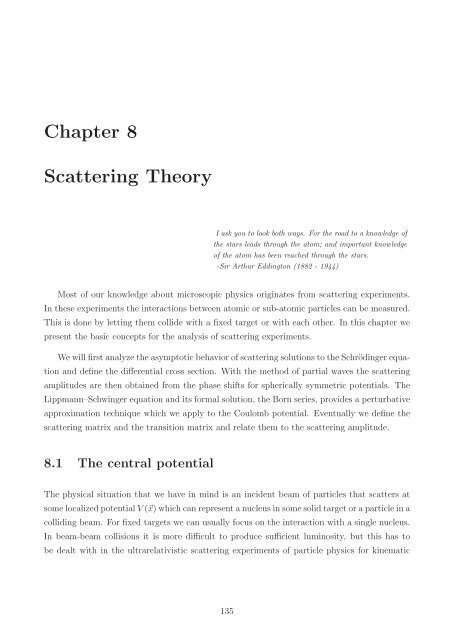
Center-of-Mass System. As shown in fig. 8.1 we denote by ⃗p 1 and ⃗p 2 the momenta<br />
of the incoming particles and of the target, respectively. The center of mass momentum is<br />
⃗p g = ⃗p 1 + ⃗p 2 = ⃗p 1L with the target at rest ⃗p 2L = 0 in the laboratory frame. As we derived<br />
1<br />
Using the notation of figure 8.1 below with an incident particle of energy E 1 = E in = √ c 2 ⃗p 2<br />
1L + m2 1 c4<br />
hitting a target with mass m 2 at rest in the laboratory system the total energy<br />
E 2 = c 2 (p 1L + p 2L ) 2 = (E 1 + m 2 c 2 ) 2 − c 2 ⃗p 2<br />
1L = m 2 1c 4 + m 2 1c 4 + 2E in m 2 c 2 (8.1)<br />
available for particle production in the center of mass system is only E ≈ √ 2E in m 2 c 2 for E in ≫ m 1 c 2 ,m 2 c 2 .<br />
0
CHAPTER 8. SCATTERING THEORY 137<br />
p 1L<br />
p ′ 1L<br />
θ L<br />
p 1 ′<br />
p 1 θ<br />
p 2<br />
p ′ 2L<br />
p 2 ′<br />
Figure 8.1: <strong>Scattering</strong> angle for fixed target and in the center of mass frame.<br />
in section 4, the kinematics of the reduced 1-body problem is given by the reduced mass<br />
µ = m 1 m 2 /(m 1 + m 2 ) and the momentum<br />
⃗p = ⃗p 1m 2 − ⃗p 2 m 1<br />
m 1 + m 2<br />
. (8.5)<br />
Obviously ϕ = ϕ L , while the relation between θ in the center of mass frame and the angle θ L<br />
in the fixed target (laboratory) frame can be obtained by comparing the momenta ⃗p ′ 1 of the<br />
scattered particles. With p i = |⃗p i | the transversal momentum is<br />
p ′ 1L sin θ L = p ′ 1 sin θ. (8.6)<br />
The longitudinal momentum is ⃗p ′ 1 cos θ in the center of mass frame. In the laboratory frame we<br />
have to add the momentum due to the center of mass motion with velocity ⃗v g , where<br />
⃗p 1L = ⃗p 1 + m 1 ⃗v g = ⃗p g = (m 1 + m 2 )⃗v g ⇒ m 2 ⃗v g = ⃗p 1 . (8.7)<br />
Restricting to elastic scattering where |⃗p 1 ′ | = |⃗p 1 | we find for the longitudinal motion<br />
We hence find the formula<br />
p ′ 1L cos θ L = p ′ 1 cos θ + m 1 v g<br />
el.<br />
= p ′ 1(cos θ + m 1<br />
m 2<br />
) (8.8)<br />
tanθ elastic<br />
L = sin θ<br />
cos θ + τ<br />
with τ = m 1<br />
m 2<br />
=<br />
m in<br />
m target<br />
(8.9)<br />
for the scattering angle in the laboratory frame for elastic scattering. According to the change<br />
of the measure of the angular integration the differential cross section also changes by a factor<br />
( )<br />
dσ<br />
(θ L (θ)) =<br />
d(cosθ)<br />
dσ<br />
dΩ ∣<br />
L<br />
d(cos θ L ) ∣ dΩ (θ) = (1 + 2τ cosθ + τ2 ) 3/2 dσ<br />
(θ) (8.10)<br />
|1 + τ cos θ| dΩ<br />
where we used cos θ L = 1/ √ 1 + tan 2 θ = (cosθ + τ)/ √ 1 + 2τ cos θ + τ 2 .<br />
8.1.2 Asymptotic expansion and scattering amplitude<br />
We now consider the scattering of a beam of particles by a fixed center of force and let m denote<br />
the reduced mass and ⃗x the relative coordinate. If the beam of particles is switched on for a<br />
long time compared to the time one particle needs to cross the interaction area, steady-state
CHAPTER 8. SCATTERING THEORY 138<br />
conditions apply and we can focus on stationary solutions of the time-independent Schrödinger<br />
equation [<br />
− 2<br />
2m ∆ + V (⃗x) ]<br />
u(⃗x) = Eu(⃗x), ψ(⃗x,t) = e −iωt u(⃗x). (8.11)<br />
The energy eigenvalues E is related by<br />
E = 1 2 m⃗v2 = ⃗p2<br />
2m = 2 ⃗ k<br />
2<br />
2m<br />
(8.12)<br />
to the incident momentum ⃗p, the incident wave vector ⃗ k and the incident velocity ⃗v. For<br />
convenience we introduce the reduced potential<br />
U(⃗x) = 2m/ 2 · V (⃗x) (8.13)<br />
so that we can write the Schrödinger equation as<br />
[∇ 2 + k 2 − U(⃗x)]u(⃗x) = 0. (8.14)<br />
For potentials that asymptotically decrease faster then r −1<br />
|V as (r)| ≤ c/r α for r → ∞ with α > 1, (8.15)<br />
we can neglect U(⃗x) for large r and the Schrödinger equation reduces to the Helmholtz equation<br />
of a free particle<br />
[∆ + k 2 ]u as (⃗x) = 0. (8.16)<br />
Potentials satisfying (8.15) are called finite range. (The important case of the Coulomb potential<br />
is, unfortunately, of infinite range, but we will be able to treat it as the limit α → 0 of the<br />
finite range Yukawa potential e −αr /r.) For large r we can decompose the wave function into a<br />
part u in describing the incident beam and a part u sc for the scattered particles<br />
u(⃗x) → u in (⃗x) + u sc (⃗x) for r → ∞. (8.17)<br />
Since we took the z-axis as the direction of incidence and since the particles have all the same<br />
momentum p = k the incident wave function can be written as<br />
u in (⃗x) = e i⃗k·⃗x = e ikz , (8.18)<br />
where we were free to normalize the amplitude of u in since all equations are linear.<br />
Far from the scattering center the scattered wave function represents an outward radial flow<br />
of particles. We can parametrize it in terms of the scattering amplitude f(k,θ,ϕ) as<br />
u sc (⃗x) = f(k,θ,ϕ) eikr<br />
r + O( 1<br />
rα), (8.19)
CHAPTER 8. SCATTERING THEORY 139<br />
where (r,θ,ϕ) are the polar coordinates of the position vector ⃗x of the scattered particle. The<br />
asymptotic form u as of the scattering solution thus becomes<br />
u as = (e i⃗ k·⃗x ) as + f(k,θ,ϕ) eikr<br />
r . (8.20)<br />
The scattering amplitude can now be related to the differential cross-section. From chapter 2<br />
we know the probability current density for the stationary state<br />
⃗j(⃗x) = <br />
2im (ψ∗ ⃗ ∇ψ − ψ ⃗ ∇ψ ∗ ) = m Re (u∗ ⃗ ∇u) (8.21)<br />
with the gradient operator in spherical polar coordinates (r,θ,ϕ) reading<br />
⃗∇ = ⃗e r<br />
∂<br />
∂r + ⃗e θ<br />
1<br />
r<br />
∂<br />
∂θ + ⃗e ϕ<br />
1<br />
r sin θ<br />
For large r the scattered particle current flows in radial direction with<br />
∂<br />
∂ϕ . (8.22)<br />
j r = k<br />
mr 2 |f(k,θ,ϕ)|2 + O( 1 r3). (8.23)<br />
Since the area of the detector is r 2 dΩ the number of particles NdΩ entering the detector per<br />
unit time is<br />
NdΩ = k m |f(k,θ,ϕ)|2 dΩ. (8.24)<br />
For |ψ in (⃗x)| 2 = 1 the incoming flux F = k/m = v is given by the particle velocity. We thus<br />
obtain the differential cross-section<br />
as the modulus squared of the scattering amplitude.<br />
dσ<br />
dΩ = |f(k,θ,ϕ)|2 (8.25)<br />
8.2 Partial wave expansion<br />
For a spherically symmetric central potential V (⃗x) = V (r) we can use rotation invariance to<br />
simplify the computation of the scattering amplitude by an expansion of the angular dependence<br />
in spherical harmonics. Since the system is completely symmetric under rotations about the<br />
direction of incident beam (chosen along the z-axis), the wave function and the scattering<br />
amplitude do not depend on ϕ. Thus we can expand both u ⃗k (r,θ) and f(k,θ) into a series of<br />
Legendre polynomials, which form a complete set of functions for the interval −1 cos θ +1,<br />
u ⃗k (r,θ) =<br />
f(k,θ) =<br />
∞∑<br />
R l (k,r)P l (cos θ), (8.26)<br />
l=0<br />
∞∑<br />
(2l + 1)f l (k)P l (cos θ), (8.27)<br />
l=0
CHAPTER 8. SCATTERING THEORY 140<br />
where the factor (2l + 1) in the definition of the partial wave amplitudes f l (k) corresponds to<br />
the degeneracy of the magnetic quantum number. (Some authors use different conventions,<br />
like either dropping the factor (2l + 1) or including an additional factor 1/k in the definition<br />
of f l .) The terms in the series (8.26) are known as a partial waves, which are simultaneous<br />
eigenfunctions of the operators L 2 and L z with eigenvalues l(l + 1) 2 and 0, respectively. Our<br />
aim is now to determine the amplitudes f l in terms of the radial functions R l (k,r) for solutions<br />
(8.27) to the Schrödinger equation.<br />
The radial equation. We recall the formula for the Laplacian in spherical coordinates<br />
∆ = 1 (<br />
∂<br />
r 2 ∂ )<br />
− L2<br />
with − L r 2 ∂r ∂r 2 r 2 = 1 (<br />
∂<br />
sin θ ∂ )<br />
+ 1 ∂ 2<br />
2 sin θ ∂θ ∂θ sin 2 (8.28)<br />
θ ∂ϕ 2<br />
With the separation ansatz<br />
u Elm (⃗x) = R El (r)Y lm (θ,ϕ) (8.29)<br />
for the time-independent Schrödinger equation with central potential in spherical coordinates<br />
[ (<br />
{− 2 1 ∂<br />
r 2 ∂ ) ] }<br />
− L2<br />
+ V (r) u(⃗x) = Eu(⃗x), (8.30)<br />
2m r 2 ∂r ∂r 2 r 2<br />
and L 2 Y lm (θ,ϕ) = l(l + 1) 2 Y lm (θ,ϕ) we find the radial equation<br />
( (− 2 d<br />
2<br />
2m dr + 2 ) )<br />
d l(l + 1)2<br />
+ + V (r) R 2 r dr 2mr 2<br />
El (r) = ER El (r). (8.31)<br />
and its reduced form<br />
( d<br />
2<br />
dr 2 + 2 r<br />
)<br />
d l(l + 1)<br />
− − U(r) + k 2 R<br />
dr r 2 l (k,r) = 0 (8.32)<br />
with k = √ 2mE/ 2 and the reduced potential U(r) = (2m/ 2 )V (r).<br />
Behavior near the center. For potentials less singular than r −2 at the origin the behavior<br />
of R l (k,r) at r = 0 can be determined by expanding R l into a power series<br />
∑ ∞<br />
R l (k,r) = r s a n r n . (8.33)<br />
Substitution into the radial equation (8.32) leads to the quadratic indicial equation with the<br />
two solutions s = l and s = −(l + 1). Only the first one leads to a non-singular wave function<br />
u(r,θ) at the origin r = 0.<br />
Introducing a new radial function ˜R El (r) = rR El (r) and substituting into (8.31) leads to<br />
the equation (<br />
− 2<br />
2m<br />
n=0<br />
)<br />
d 2<br />
dr + V eff(r) ˜R 2 El (r) = E ˜R El (r) (8.34)
CHAPTER 8. SCATTERING THEORY 141<br />
which is similar to the one-dimensional Schrödinger equation but with r ≥ 0 and an effective<br />
potential<br />
l(l + 1)2<br />
V eff = V (r) + (8.35)<br />
2mr 2<br />
containing the repulsive centrifugal barrier term l(l + 1) 2 /2mr 2 in addition to the interaction<br />
potential V (r).<br />
Free particles and asymptotic behavior. We now solve the radial equation for V (r) = 0<br />
so that our solutions can later be used either for the representation of the wave function of a free<br />
particle at any radius 0 ≤ r < ∞ or for the asymptotic form as r → ∞ of scattering solutions<br />
for finite range potentials. Introducing the dimensionless variable ρ = kr with R l (ρ) = R El (r)<br />
for U(r) = 0 the radial equation (8.31) turns into the spherical Bessel differential equation<br />
[ d<br />
2<br />
dρ + 2 ( )]<br />
d<br />
2 ρ dρ + l(l + 1)<br />
1 − R<br />
ρ 2 l (ρ) = 0, (8.36)<br />
whose independent solutions are the spherical Bessel functions<br />
and the spherical Neumann functions<br />
( ) l 1<br />
j l (ρ) = (−ρ) l d sin ρ<br />
ρ dρ ρ<br />
(8.37)<br />
Their leading behavior at ρ = 0,<br />
( ) l 1<br />
n l (ρ) = −(−ρ) l d cos ρ<br />
ρ dρ ρ . (8.38)<br />
lim j l(ρ) →<br />
ρ→0<br />
ρ l<br />
1 · 3 · 5 · ... · (2l + 1) , (8.39)<br />
lim n 1 · 3 · 5 · ... · (2l − 1)<br />
l(ρ) → − (8.40)<br />
ρ→0 ρ l+1<br />
can be obtained by expanding ρ −1 sin ρ and ρ −1 cos ρ into a power series in ρ. In accord with our<br />
previous result for the ansatz (8.33) the spherical Neumann function n l (ρ) has a pole of order<br />
l + 1 at the origin and is therefore an irregular solution, whereas the spherical Bessel function<br />
j l (ρ) is the regular solution with a zero of order l at the origin. The radial part of the wave<br />
function of a free particle can hence only contain spherical bessel functions R free<br />
El<br />
(r) ∝ j l (kr).<br />
8.2.1 Expansion of a plane wave in spherical harmonics<br />
In order to use the spherical symmetry of a potential V (r) we need to expand the plane wave<br />
representing the incident particle beam in terms of spherical harmonics. Since e i⃗ k·⃗x is a regular<br />
solution to the free Schrödinger equation we can make the ansatz<br />
e i⃗ k·⃗x =<br />
∞∑<br />
∑+l<br />
l=0 m=−l<br />
c lm j l (kr)Y lm (θ,ϕ), (8.41)
CHAPTER 8. SCATTERING THEORY 142<br />
where the radial part is given by the spherical Bessel functions with constants c lm that have<br />
to be determined. Choosing ⃗ k in the direction of the z-axis the wave function exp(i ⃗ k · ⃗r) =<br />
exp(ikr cosθ) is independent of ϕ so that only the Y lm with m = 0, which are proportional to<br />
the Legendre polynomials P l (θ), can contribute to the expansion<br />
e ikr cos θ =<br />
∞∑<br />
a l j l (kr)P l (cos θ). (8.42)<br />
l=0<br />
With ρ = kr and u = cos θ this becomes<br />
e iρu =<br />
∞∑<br />
a l j l (ρ)P l (u). (8.43)<br />
l=0<br />
One way of determining the coefficients a l is to differentiate this ansatz with respect to ρ,<br />
iue iρu = ∑ l<br />
a l<br />
dj l<br />
dρ P l. (8.44)<br />
The left hand side of (8.44) can now be evaluated by inserting the series (8.43) and using the<br />
recursion relation<br />
(2l + 1)uP m<br />
l<br />
of the Legendre polynomials for m = 0. This yields<br />
i<br />
∞∑<br />
l=0<br />
= (l + 1 − m)P m<br />
l+1 + (l + m)P m<br />
l−1 (8.45)<br />
( l + 1<br />
a l j l<br />
2l + 1 P l+1 +<br />
l )<br />
2l + 1 P l−1 =<br />
∞∑<br />
a l j lP ′ l (8.46)<br />
and, since the Legendre polynomials are linearly independent, for the coefficient of P l<br />
( l<br />
a l j l ′ = i<br />
2l − 1 a l−1j l−1 + l + 1 )<br />
2l + 3 a l+1j l+1 . (8.47)<br />
The derivative j l ′ can now be expressed in terms of j l±1 by using the recursion relations<br />
( d<br />
j l−1 =<br />
dρ + l + 1 )<br />
j l = 1 d<br />
ρ ρ l+1 dρ (ρl+1 j l ) (8.48)<br />
l=0<br />
and<br />
(2l + 1)j l = ρ[j l+1 + j l−1 ], (8.49)<br />
which imply<br />
j ′ l = j l−1 − l + 1<br />
ρ j l = j l−1 − l + 1<br />
2l + 1 (j l+1 + j l−1 ) =<br />
l<br />
2l + 1 j l−1 − l + 1<br />
2l + 1 j l+1 (8.50)<br />
[the equations (8.48-8.50) also holds for the spherical Neumann functions n l ]. Substituting this<br />
expression for j ′ l<br />
into eq. (8.47) we obtain the two equivalent recursion relations<br />
a l<br />
2l + 1 = i a l−1<br />
2l − 1<br />
and<br />
a l<br />
2l + 1 = −i a l+1<br />
2l + 3<br />
(8.51)
CHAPTER 8. SCATTERING THEORY 143<br />
as coefficients of the independent functions j l−1 (ρ) and j l+1 (ρ), respectively. These relations<br />
have the solution a l = (2l + 1)i l a 0 . The coefficient a 0 is obtained by evaluating our ansatz at<br />
ρ = 0: Since j l (0) = δ l0 and P 0 (u) = 1 eq. (8.43) implies a 0 = 1, so that the expansion of a<br />
plane wave in spherical harmonics becomes<br />
e ikr cos θ =<br />
∞∑<br />
(2l + 1)i l j l (kr)P l (cosθ). (8.52)<br />
l=0<br />
Using the addition theorem of spherical harmonics<br />
2l + 1<br />
4π P l(cos α) =<br />
∑+l<br />
m=−l<br />
Y ∗<br />
lm(θ 1 ,ϕ 1 )Y lm (θ 2 ,ϕ 2 ) (8.53)<br />
with α being the angle between the directions (θ 1 ,ϕ 1 ) and (θ 2 ,ϕ 2 ) this result can be generalized<br />
to the expansion of the plane wave in any polar coordinate system<br />
e i⃗ k·⃗x = 4π<br />
∞∑<br />
∑+l<br />
l=0 m=−l<br />
i l j l (kr)Y ∗<br />
lm(θ ⃗k ,ϕ ⃗k )Y lm (θ ⃗x ,ϕ ⃗x ), (8.54)<br />
where the arguments of Y ∗<br />
lm and Y lm are the angular coordinates of ⃗ k and ⃗x, respectively.<br />
8.2.2 <strong>Scattering</strong> amplitude and phase shift<br />
The computation of the scattering data for a given potential requires the construction of the<br />
regular solution of the radial equation. In the next section we will solve this problem for the<br />
example of the square well, but first we analyse the asymptotic form of the partial waves in<br />
order to find out how to extract and interpret the relevant data.<br />
For large r we can neglect the potential U(r) and it is common to write the asymptotic form<br />
of the radial solutions as a linear combination of the spherical Bessel and Neumann functions<br />
R l (k,r) = B l (k)j l (kr) + C l (k)n l (kr) + O(r −α ) (8.55)<br />
with coefficients B l (k) and C l (k) that depend on the incident momentum k. Inserting the<br />
asymptotic forms<br />
we can write<br />
j l (kr) = 1 (kr<br />
kr sin − lπ )<br />
2<br />
n l (kr) = − 1 (kr<br />
kr cos − lπ )<br />
2<br />
Rl as (k,r) = 1 [ (<br />
B l (k) sin kr − lπ )<br />
kr<br />
2<br />
= A l (k) 1<br />
kr sin (<br />
kr − lπ 2 + δ l(k)<br />
+ O( 1 r2), (8.56)<br />
+ O( 1 r2), (8.57)<br />
(<br />
− C l (k) cos<br />
)<br />
kr − lπ 2<br />
)]<br />
(8.58)<br />
(8.59)
CHAPTER 8. SCATTERING THEORY 144<br />
where<br />
and<br />
A l (k) = [B 2 l (k) + C 2 l (k)] 1/2 (8.60)<br />
δ l (k) = − tan −1 [C l (k)/B l (k)]. (8.61)<br />
The δ l (k) are called phase shifts. We will see that they are real functions of k and completely<br />
characterize the strength of the scattering of the lth partial wave by the potential U(r) at the<br />
energy E = 2 k 2 /2m. In order to relate the phase shifts to the scattering amplitude we now<br />
insert the asymptotic form of the expansion (8.52) of the plane wave<br />
e i⃗ k⃗x<br />
=<br />
→<br />
∞∑<br />
(2l + 1)i l j l (kr)P l (cos θ). (8.62)<br />
l=0<br />
∞∑<br />
(2l + 1)i l (kr) −1 sin<br />
l=0<br />
(<br />
kr − lπ )<br />
P l (cos θ). (8.63)<br />
2<br />
into the scattering ansatz (8.20)<br />
u as<br />
⃗ k<br />
(r,θ) → e i⃗ k⃗x + f(k,θ) eikr<br />
r . (8.64)<br />
With sin x = (e ix −e −ix )/(2i) and the partial wave expansions (8.26)–(8.27) of u(⃗x) and f(θ,ϕ)<br />
we can write the radial function R l (k,r), i.e. the coefficient of P l (cos θ), asymptotically as<br />
(<br />
Rl as (k,r) = (2l + 1)i l (kr) −1 sin kr − lπ )<br />
+ 2l + 1 e ikr f l (k) (8.65)<br />
2 r<br />
= 2l + 1 ( ) )<br />
e<br />
(i l ikr<br />
− e−ikr<br />
+ 2ike ikr f<br />
2ikr i l (−i) l l (8.66)<br />
Rewriting (8.59) in terms of exponentials<br />
Rl as (k,r) = A (<br />
l e<br />
i(kr+δ l<br />
)<br />
)<br />
− e−i(kr+δ l)<br />
2ikr i l (−i) l<br />
(8.67)<br />
comparison of the coefficients of e −ikr implies<br />
A l (k) = (2l + 1)i l e iδ l(k) . (8.68)<br />
The coefficients of e ikr /(2ikr) are (2l + 1)(1 + 2ikf l ) and A l e iδ l /i l , respectively. Hence<br />
f l (k) = e2iδ l(k) − 1<br />
2ik<br />
= 1 k eiδ l<br />
sin δ l . (8.69)<br />
The scattering amplitude<br />
f(k,θ) =<br />
∞∑<br />
l=0<br />
(2l + 1)f l (k)P l (cos θ) = 1<br />
2ik<br />
∞∑<br />
(2l + 1)(e 2iδ l<br />
− 1)P l (cos θ) (8.70)<br />
l=0
CHAPTER 8. SCATTERING THEORY 145<br />
hence depends only on the phase shifts δ l (k) and the asymptotic form of R l (k,r) takes the form<br />
Rl as (k,r) = − 1 [ ]<br />
2ik A l(k)e −iδ l(k) e<br />
−i(kr−lπ/2)<br />
− S l (k) ei(kr−lπ/2)<br />
(8.71)<br />
r<br />
r<br />
where we defined<br />
S l (k) = e 2iδ l(k) . (8.72)<br />
S l is the partial wave contribution to the S-matrix, which we will introduce in the last section of<br />
this chapter. Reality of the phase shift |S l | = 1 expresses equality of the incoming and outgoing<br />
particle currents, i.e. conservation of particle number or unitarity of the S matrix. For inelastic<br />
scattering we could write the radial wave fuction as (8.71) with S l = s l e iδ l for sl ≤ 1 describing<br />
the loss of part of the incoming current into inelastic processes like energy transfer of particle<br />
production. (The complete scattering matrix, including the contribution of inelastic channels,<br />
would however still be unitary as a consequence of the conservation of probability.)<br />
The optical theorem. The total cross section for scattering by a central potential can be<br />
written as<br />
∫<br />
σ tot =<br />
|f(k,θ)| 2 dΩ = 2π<br />
∫ +1<br />
−1<br />
d(cos θ)f ∗ (k,θ)f(k,θ). (8.73)<br />
Using (8.70) and the orthogonality property of the Legendre polynomials<br />
∫ +1<br />
−1<br />
d(cosθ)P l (cosθ)P l ′(cosθ) = 2<br />
2l + 1 δ ll ′ (8.74)<br />
we find<br />
σ tot =<br />
∞∑<br />
4π(2l + 1)|f l (k)| 2 =<br />
l=0<br />
∞∑<br />
l=0<br />
σ l with σ l = 4π<br />
k 2 (2l + 1) sin2 δ l . (8.75)<br />
Since (8.69) implies Imf l = k|f l | 2 we can set θ = 0 in (8.70) and use the fact that P l (1) = 1 to<br />
obtain the optical theorem<br />
σ tot = 4π Imf(k,θ = 0), (8.76)<br />
k<br />
The optical theorem can be shown to hold also for inelastic scattering with σ tot = σ el + σ inel .<br />
The proof relates the total cross section to the interference of the incoming with the forwardscattered<br />
amplitude so that (8.76) is a consequence of the unitarity of the S-matrix [Hittmair].<br />
8.2.3 Example: <strong>Scattering</strong> by a square well<br />
The centrally symmetric square well is a potential for which the phase shifts can be calculated<br />
by analytical methods. Starting with the radial equation (8.32) and the reduced potential<br />
{ −U0 , r < a (U<br />
U(r) =<br />
0 > 0)<br />
0, r > a,<br />
(8.77)
CHAPTER 8. SCATTERING THEORY 146<br />
we can write the radial equation inside the well as<br />
[ d<br />
2<br />
dr + 2 ]<br />
d l(l + 1)<br />
− + K 2 R 2 r dr r 2 l (k,r) = 0 for r < a (8.78)<br />
with K 2 = k 2 + U 0 . Inside the well the regular solution is thus<br />
R in<br />
l (K,r) = N l j l (Kr), r < a (8.79)<br />
where N l is related to the exact solution in the exterior region<br />
R ext<br />
l (k,r) = B l (k)[j l (kr) − tanδ l (k)n l (kr)], r > a (8.80)<br />
by the matching condition at r = a. Continuity of R and R ′ at r = a hence implies<br />
N l j l (Ka) = B l (j l (ka) − tanδ l n l (ka)), (8.81)<br />
KN l j ′ l(Ka) = kB l (j ′ l(ka) − tanδ l n ′ l(ka)). (8.82)<br />
The ratio of these two equations yields an equation for tanδ l (k) whose solution is<br />
with K = √ k 2 + U 0 .<br />
tanδ l (k) = kj′ l (ka)j l(Ka) − Kj l (ka)j ′ l (Ka)<br />
kn ′ l (ka)j l(Ka) − Kn l (ka)j ′ l (Ka) (8.83)<br />
In the low energy limit k = √ 2mE/ → 0 we can insert the leading behavior j l (ρ) ∝ ρ l<br />
and n l (ρ) ∝ ρ −l−1 , and thus for the derivatives j ′ l (ρ) ∝ ρl−1 and n ′ l (ρ) ∝ ρ−l−2 , to conclude that<br />
tanδ l (k) goes to zero like a constant times k l /k −l−1 = k 2l+1 . In this limit the cross section,<br />
σ l ∝ k 4l , (8.84)<br />
is dominated by l = 0 so that the scattering probability approximately goes to a θ-independent<br />
constant. With<br />
j 0 (ρ) = sin ρ<br />
ρ ,<br />
n 0(ρ) = − cos ρ<br />
ρ ,<br />
j′ 0(ρ) =<br />
ρcos ρ−sin ρ<br />
ρ 2 , n ′ 0(ρ) =<br />
ρsin ρ+cos ρ<br />
ρ 2 (8.85)<br />
and the abbreviations x = ka, X = Ka we find<br />
tan δ 0 =<br />
((xcos x−sin x) sin X−sin x(X cos X−sin X))/(xX)<br />
(xsin x+cos x) sin X+cos x(X cos X−sin X))/(xX)<br />
Dividing numerator and denominator by cosxcos X we obtain the result<br />
tanδ 0 (k) =<br />
=<br />
xcos xsin X−X sin x cos X<br />
xsin x sin X+X cos x cos X . (8.86)<br />
k tan(Ka) − K tan(ka)<br />
K + k tan(ka) tan(Ka) . (8.87)<br />
For k → 0 we observe that tanδ 0 becomes proportial to k. The limit<br />
a s = − lim<br />
k→0<br />
tanδ 0 (k)<br />
k<br />
(8.88)
CHAPTER 8. SCATTERING THEORY 147<br />
is called scattering length and it determines the limit of the partial cross section<br />
σ 0 = 4π<br />
k 2 sin2 δ 0 = 4π<br />
k 2 1<br />
1 + cot 2 δ 0 (k)<br />
k→0<br />
−→ 4πa 2 s. (8.89)<br />
For the square well we find<br />
a s =<br />
The coefficient of the next term of the expansion<br />
(<br />
1 − tan(a√ )<br />
U 0 )<br />
a √ a, (8.90)<br />
U 0<br />
k cotδ 0 (k) = − 1 a s<br />
+ 1 2 r 0k 2 + · · · (8.91)<br />
defines the effective range r 0 . This definition of the scattering length a s and the effective range<br />
r 0 can be used for all short-range potentials.<br />
Another exactly solvable potential is the hard-sphere potential<br />
U(r) =<br />
{ +∞, r < a,<br />
0, r > a,<br />
(8.92)<br />
for which the total cross section can be shown to obey<br />
σ(k) →<br />
{ 4πa 2 , k → 0,<br />
2πa 2 , k ≫ 1/a.<br />
(8.93)<br />
For k → 0 the scattering length a s hence coincides with a and the cross section is 4 times<br />
the classical value. For ka ≫ 1 the wave lengths of the scattered particles goes to 0 and one<br />
might naively expect to observe the classical area a 2 π. The fact that quantum mechanics yield<br />
twice that value is in accord with refraction phenomena in optics and can be attributed to<br />
interference between the incoming and the scattered beam close to the forward direction. This<br />
effect is hence called refraction scattering, or shadow scattering.<br />
8.2.4 Interpretation of the phase shift<br />
For a weak and slowly varying potential we may think of the phase shift as arising from the<br />
change in the effective wavelength k ∼ √ 2m(E − V (x))/ due to the presence of the potential.<br />
For an attractive potential we hence expect an advanced oscillation and a positive phase shift<br />
δ l > 0, while a repulsive potential should lead to retarded oscillation and a negative phase<br />
shift δ l < 0. Comparing this expectation with the result (8.90) for the square well and using<br />
tanx ≈ x + 1 3 x3 for small U 0 we find a s ≈ − 1 3 a3 U 0 so that indeed the scattering length (8.88)<br />
becomes negative and the phase shift δ 0 positive for an attractive potential U 0 > 0. It can also<br />
be shown quite generally that small angular momenta dominate the scattering at low energies<br />
and that the partial cross sections σ l are negligible for l > ka where a is the range of the<br />
potential.
CHAPTER 8. SCATTERING THEORY 148<br />
Figure 8.2: Z boson resonance in e + e − scattering at LEP and light neutrin number.<br />
As we increase the energy the phase shift varies and the partial cross sections<br />
σ l (E) = 4π<br />
k 2 (2l + 1) sin2 δ l = 4π<br />
k 2 (2l + 1) 1<br />
1 + cot 2 δ l<br />
(8.94)<br />
go through maxima and zeros as the phase shift δ l goes through odd and even multiples of π,<br />
respectively. For small energies the single cross section σ 0 dominates so that we can get minima<br />
where the target becomes almost transparent. This is called Ramsauer-Townsend effect.<br />
A rapid move of the phase shift through an odd multiple of π, i.e.<br />
cot δ l ≈ ( (n + 1)π − δ ) E R − E<br />
2 l ≈<br />
Γ(E)/2 + O(E R − E) 2 for δ l ≈ (n + 1 )π (8.95)<br />
2<br />
with Γ(E R ) small at the resonance energy E R , leads to a sharp peak in the cross section with an<br />
angular distibution characteristic for the angular momentum chanel l. This is called resonance<br />
scattering and described by the Breit-Wigner resonance formula<br />
σ l (E) = 4π<br />
k 2 (2l + 1) Γ 2 /4<br />
(E − E R ) 2 + Γ 2 /4 . (8.96)<br />
A resonance can be thought of as a metastable bound state with positive energy whose lifetime<br />
is /Γ. For a sharp resonance the inverse width Γ −1 is indeed related to the dwelling time of<br />
the scattered particles in the interaction region. Note that σ max at a resonance is determined<br />
by the momentum k of the scattered particles and not by properties of the target. A striking<br />
example of a resonance in particle physics is the peak in electron-positron scattering at the<br />
Z-boson mass which was analyzed by the LEP-experiment ALEPH as shown in fig. 8.2. Since<br />
the Z boson has no electric charge but couples to the weakly interacting particles its lifetime is<br />
very sensitive to the number of light neutrinos, which are otherwise extremely hard to observe.<br />
This experiment confirmed with great precision the number N ν = 3 of such species, which is<br />
also required for nucleosynthesis, about one second after the big bang, to produce the right<br />
amount of helium and other light elements as observed in the interstellar gas clouds.
CHAPTER 8. SCATTERING THEORY 149<br />
Resonances can be interpreted as poles in the scattering amplitudes that are close to the<br />
real axis (with the imaginary part related to the lifetime). Poles on the positive imaginary axis,<br />
on the other hand, correspond to bound states for the potential V (x). The information of the<br />
number of such bound states is also contained in the phase shift. For the precise statement we<br />
fix the ambiguity modulo 2π in the definition (8.61) of δ l by requiring continuity. The Levinson<br />
theorem then states that<br />
δ l (0) − δ l (∞) = n l π for l > 0, (8.97)<br />
where n l denotes the number of bound states with angular momentum l [Chadan-Sabatier].<br />
The theorem also holds for l = 0 except for a shift n l → n l + 1 in the formula (8.97) if there is a<br />
2<br />
so-called bound state a zero energy with l = 0. While we consider in this chapter the problem of<br />
determining the scattering data from the potential, in inverse problem of obtaining information<br />
on the potential from the scattering data is physically equally important, but mathematically<br />
quite a bit more complicated. Inverse scattering theory has been a very active field of research<br />
in the last decades with a number of interesting interrelations to other fields like integrable<br />
systems [Chadan-Sabatier].<br />
8.3 The Lippmann-Schwinger equation<br />
We can use the method of Green’s functions to solve the stationary Schrödinger equation (8.14)<br />
(∇ 2 + k 2 )u(⃗x) = U(⃗x)u(⃗x). (8.98)<br />
Using the defining equation of the Green’s function for the Helmholtz equation<br />
(∇ 2 + k 2 )G 0 (k,⃗x,⃗x ′ ) = δ(⃗x − ⃗x ′ ) (8.99)<br />
we can write down the general solution of equation (8.98) as a convolution integral<br />
∫<br />
u(⃗x) = u hom (⃗x) + G 0 (k,⃗x,⃗x ′ )U(⃗x ′ )u(⃗x ′ ) d 3 x ′ (8.100)<br />
where u hom is a solution of the homogenous Schrödinger equation<br />
(∇ 2 + k 2 )u hom (⃗x) = 0. (8.101)<br />
We will see that the scattering boundary condition (8.20) is equivalent to taking u hom (⃗x) to be<br />
an incident plane wave<br />
u hom (⃗x) = φ ⃗k (⃗x) ≡ e i⃗ k⃗x<br />
(8.102)<br />
if G 0 = G ret<br />
0 is the retarded Green’s function. The existence of solutions to the homogeneous<br />
equation is of course related to the ambiguity of G 0 , as we will see explicitly in the following<br />
computation.
CHAPTER 8. SCATTERING THEORY 150<br />
Since (8.99) is a linear differential equation with constant coefficients we can determine the<br />
Green’s function by Fourier transformation. Because of translation invariance<br />
G 0 (k,⃗x,⃗x ′ ) = G 0 (k, ⃗ R) with ⃗ R = ⃗x − ⃗x ′ , (8.103)<br />
hence<br />
G 0 (k,⃗x − ⃗x ′ ) =<br />
δ(⃗x − ⃗x ′ ) =<br />
∫<br />
1<br />
(2π) 3 ∫<br />
1<br />
(2π) 3<br />
e i ⃗ K·⃗R ˜g 0 (k, ⃗ K)d ⃗ K (8.104)<br />
e i ⃗ K·⃗R d ⃗ K. (8.105)<br />
Substituting the Fourier representations into the defining equation of the Green’s function<br />
(8.99) we find that<br />
˜g 0 (k, K) ⃗ 1<br />
=<br />
k 2 − K2. (8.106)<br />
Since ˜g 0 has a pole on the real axis we give a small imaginary part to k and define<br />
G ± 0 (k,⃗x,⃗x ′ ) = 1<br />
(2π) 3 ∫<br />
e i ⃗ K·(⃗x−⃗x ′ )<br />
k 2 − K 2 ± iε d ⃗ K. (8.107)<br />
Let (K, Θ, Φ) be the spherical coordinates of ⃗ K and let the z-axis be along ⃗ R = ⃗x − ⃗x ′ . Then<br />
G ± 0 (k, R) ⃗ = 1 ∫ ∞ ∫ π<br />
dKK 2<br />
(2π) 3<br />
0<br />
0<br />
∫ 2π<br />
dΘ sin Θ<br />
0<br />
cos Θ<br />
eiKR<br />
dΦ<br />
k 2 − K 2 ± iε . (8.108)<br />
Performing the angular integrations and observing that the integrand is an even function of K<br />
we can extend the integral from −∞ to +∞ and obtain<br />
G ± 0 (k, ⃗ R) = 1<br />
8π 2 iR<br />
∫ +∞<br />
−∞<br />
K(e iKR − e −iKR ))<br />
dK. (8.109)<br />
k 2 − K 2 ± iε<br />
(<br />
1<br />
With the partial fraction decomposition = − 1 1<br />
+ 1<br />
k 2 −K 2 2K K−k K+k)<br />
we can split the integral<br />
into two parts<br />
i<br />
G 0 (k,R) =<br />
16π 2 R (I 1 − I 2 ), (8.110)<br />
with<br />
I 1 =<br />
I 2 =<br />
∫ +∞<br />
−∞<br />
∫ +∞<br />
−∞<br />
( 1<br />
e iKR K − k + 1 )<br />
K + k<br />
e −iKR ( 1<br />
K − k + 1<br />
K + k<br />
dK (8.111)<br />
)<br />
dK (8.112)<br />
The integrals can now be evaluated using the Cauchy integral formula if we close the integration<br />
path with a half-circle in the upper or lower complex half-plane, respectively, so that the<br />
contribution from the arcs at infinity vanish. The ambiguity of the Green’s function arises<br />
from different choices of the integration about the poles of the integrand on the real axis, and<br />
different pole prescriptions obviously differ by terms localized at K 2 = k 2 and hence by a
CHAPTER 8. SCATTERING THEORY 151<br />
(a)<br />
ImK<br />
C 1<br />
P<br />
x<br />
-k<br />
x<br />
+k<br />
ReK<br />
(b)<br />
x<br />
-k<br />
ImK<br />
P<br />
x<br />
+k<br />
ReK<br />
C 2<br />
Figure 8.3: (a) The contour (P+C 1 ) for calculating the integral I 1 by avoiding the poles K = ±k<br />
and closing via a semi-circle in infinity. (b) the contour for calculating the integral I 2 .<br />
superposition of plane wave solutions to the homogeneous equation. The integration contour<br />
in the complex K-plane shown in fig. 8.3 corresponds to a small positive imaginary part of k<br />
and hence to G + 0 . Since e iKR vanishes on C 1 and e −iKR vanishes on C 2 we find<br />
I 1 = 2πie ikR (8.113)<br />
I 2 = −2πie ikR (8.114)<br />
With a similar calculation for k → k − iε the Green’s function in the original variables ⃗x and<br />
⃗x ′ becomes<br />
G ± 0 (k,⃗x,⃗x ′ ) = − 1 ±e ik|⃗x−⃗x′ |<br />
4π |⃗x − ⃗x ′ | . (8.115)<br />
so that G + 0 = G ret<br />
0 corresponds to retarded boundary conditions. With U = 2m<br />
2 V we can now<br />
write the integral equation for the wave function as<br />
u ⃗k (⃗x) = e i⃗ k·⃗x −<br />
m<br />
2π 2 ∫ e<br />
ik|⃗x−⃗x ′ |<br />
|⃗x − ⃗x ′ | V (⃗x′ )u ⃗k (⃗x ′ )d⃗x ′ . (8.116)<br />
This integral equation is known as the Lippmann-Schwinger equation for potential scattering.<br />
It is equivalent to the Schrödinger equation plus the scattering boundary condition (8.20).
CHAPTER 8. SCATTERING THEORY 152<br />
We can now relate this integral representation to the scattering amplitude by considering<br />
the situation where the distance of the detector r → ∞ is much larger than the range of the<br />
potential to which the integration variable ⃗x ′ is essentially confined so that r ′ ≪ r. Hence<br />
|⃗x − ⃗x ′ | = √ r 2 − 2⃗x⃗x ′ + r ′2 = r − ⃗x⃗x′<br />
r + O(1 ). (8.117)<br />
r<br />
Since ⃗x points in the same direction (θ,ϕ) as the wave vector ⃗ k ′ of the scattered particles we<br />
have ⃗ k ′ = k⃗x/r for elastic scattering and hence<br />
e ik|⃗x−⃗x′ |<br />
|⃗x − ⃗x ′ | −−−→<br />
r→∞<br />
e ikr<br />
r e−i⃗ k ′·⃗x ′ + · · · , (8.118)<br />
where terms of order in 1/r 2 have been neglected. Substituting this expansion into the Lippmann-<br />
Schwinger equation we find<br />
u ⃗k (⃗x) −−−→<br />
r→∞ ei⃗ k·⃗x − 1 e ikr<br />
4π r<br />
∫<br />
e −i⃗ k ′·⃗x ′ U(⃗x ′ )u ⃗k (⃗x ′ )d⃗x ′ . (8.119)<br />
Comparing with the ansatz (8.20) we thus obtain the integral representation<br />
f(k,θ,φ) = − 1 ∫<br />
e −i⃗ k ′·⃗x U(⃗x)u ⃗k (⃗x)d⃗x<br />
4π<br />
= − 1<br />
4π 〈φ ⃗ k ′|U|u ⃗k 〉 = − m<br />
2π 〈φ 2 ⃗ k ′|V |u ⃗k 〉 (8.120)<br />
for the scattering amplitude, where 〈φ ⃗k ′| = e −i⃗ k ′·⃗x and |φ ⃗k ′〉 = e i⃗ k ′·⃗x = (2π) 3/2 |k ′ 〉.<br />
8.4 The Born series<br />
The Born series is the iterative solution of the Lippmann-Schwinger equation by the ansatz<br />
∞∑<br />
u(⃗x) = u n (⃗x) for u 0 (⃗x) = φ ⃗k (⃗x) = e i⃗k·⃗x , (8.121)<br />
n=0<br />
which yields<br />
u 1 (⃗x) =<br />
∫<br />
G + 0 (k,⃗x,⃗x ′ )U(⃗x ′ )u 0 (⃗x ′ )d⃗x ′ , (8.122)<br />
.<br />
u n (⃗x) =<br />
∫<br />
G + 0 (k,⃗x,⃗x ′ )U(⃗x ′ )u n−1 (⃗x ′ )d⃗x ′ , (8.123)<br />
so that the n th term u n is formally of order O(V n ). It usually converges well for weak potentials<br />
or at high energies. Insertion of the Born series into of the formula (8.120) yields<br />
f = − 1<br />
4π 〈φ ⃗ k ′|U + UG + 0 U + UG + 0 UG + 0 U + · · · |φ ⃗k 〉 (8.124)
CHAPTER 8. SCATTERING THEORY 153<br />
and keeping only the first term we obtain the (first) Born approximation<br />
to the scattering amplitude.<br />
f B = − 1<br />
4π 〈φ ⃗ k ′|U|φ ⃗k 〉. (8.125)<br />
Phase shift in Born approximation. The Lippmann Schwinger equation (8.116) can<br />
also be analysed using partial waves. We assume that our potential is centrally symmetric and<br />
expand the scattering wave function u ⃗k in Legendre polynomials (see equation (8.26)). With<br />
the normalisation<br />
R l (k,r) −−−→ j l(kr) − tanδ l (k)n l (kr) (8.126)<br />
r→∞<br />
[ (<br />
1<br />
−−−→ sin kr − lπ ) (<br />
+ tanδ l (k) cos kr − lπ )]<br />
, (8.127)<br />
r→∞ kr 2<br />
2<br />
we find that each radial function satisfies the radial integral equation<br />
where<br />
R l (k,r) = j l (kr) +<br />
∫ ∞<br />
0<br />
G l (k,r,r ′ )U(r ′ )R l (k,r ′ )r ′2 dr ′ , (8.128)<br />
G l = kj l (kr < )n l (kr > ) with r < ≡ min(r,r ′ ) and r > ≡ max(r,r ′ ) (8.129)<br />
is the partial wave contribution to the Green’s function<br />
e ik|⃗x−⃗x′ | ∞<br />
|⃗x − ⃗x ′ | = ik ∑ (<br />
)<br />
(2l + 1)j l (kr < ) j l (kr > ) + in l (kr > ) P l (cos θ). (8.130)<br />
l=0<br />
We solve this equation by iteration, starting with R (0)<br />
l<br />
(k,r) = j l (kr). When we analyse equation<br />
(8.128) for r → ∞ we obtain the integral representation<br />
tan δ l (k) = −k<br />
∫ ∞<br />
0<br />
j l (kr)U(r)R l (k,r)r 2 dr. (8.131)<br />
Substituting the iteration for R l into the integral equation yields a Born series whose first term<br />
tanδ B l (k) = −k<br />
is the first Born approximation to tanδ l .<br />
∫ ∞<br />
0<br />
[j l (kr)] 2 U(r)r 2 dr. (8.132)<br />
Total scattering cross section in first Born approximation. With the wave vector<br />
transfer<br />
⃗q = ⃗ k − ⃗ k ′ (8.133)
CHAPTER 8. SCATTERING THEORY 154<br />
the first Born approximation of the scattering amplitude can be written as the Fourier transform<br />
f B = − 1 ∫<br />
e i⃗q·⃗x U(⃗x)d⃗x (8.134)<br />
4π<br />
of the potential. For elastic scattering with k = k ′ and ⃗ k · ⃗k ′ = k 2 cos θ we find<br />
q = 2k sin θ 2 , (8.135)<br />
with θ being the scattering angle. For a central potential it is now useful to introduce polar<br />
coordinates with angles (α,β) such that ⃗q is the polar axis. We thus find that<br />
f B (q) = − 1<br />
4π<br />
= − 1 2<br />
= − 1 q<br />
∫ ∞<br />
0<br />
∫ ∞<br />
0<br />
∫ ∞<br />
0<br />
drr 2 U(r)<br />
drr 2 U(r)<br />
∫ π<br />
0<br />
∫ +1<br />
−1<br />
dα sin α<br />
∫ 2π<br />
0<br />
iqr cos α<br />
d(cos α)e<br />
iqr cos α<br />
dβe<br />
r sin(qr)U(r)dr (8.136)<br />
only depends on q(k,θ). The total cross-section in the first Born approximation hence becomes<br />
∫ π<br />
σtot(k) B = 2π |f B (q)| 2 sin θdθ = 2π ∫ 2k<br />
|f B (q)| 2 qdq (8.137)<br />
0<br />
k 2 0<br />
where we used the differential dq = k cos θ 2 dθ of (8.135) and sinθ dθ = 2 sin θ 2 cos θ 2 dθ = q k<br />
dq<br />
k .<br />
8.4.1 Application: Coulomb scattering and the Yukawa potential<br />
Since the Coulomb potential has infinite range we apply the Born approximation to the Yukawa<br />
potential<br />
U(r) = C e−αr<br />
= C e−r/a<br />
with a = α −1 , (8.138)<br />
r r<br />
which can be regarded as a screened Colomb potential. At the end of the calculation we can<br />
then try to send the screening length a → ∞. For the Born approximation (8.136) we obtain<br />
f B = − 1 q<br />
∫ ∞<br />
0<br />
r sin(qr) C r e−αr dr = − C ∫ ∞<br />
q Im e iqr−αr dr = − C q Im 1<br />
α − iq = − C (8.139)<br />
α 2 + q 2<br />
and the corresponding differential cross section<br />
of the Yukawa potential.<br />
0<br />
dσ B<br />
dΩ = C 2<br />
(α 2 + q 2 ) 2 (8.140)<br />
The Coulomb potential. The electrostatic force between charges Q A and Q B corresponds<br />
to the potential<br />
V Coulomb (r) = Q AQ B 1<br />
4πε 0 r<br />
(8.141)
CHAPTER 8. SCATTERING THEORY 155<br />
which corresponds to<br />
C = 2m Q A Q B<br />
(8.142)<br />
2 4πε 0<br />
but obviously violates the finite range condition. Nevertheless, there is a finite limit α → 0 for<br />
which we obtain the scattering amplitude f B = −C/q 2 and the differential cross-section in first<br />
Born approximation as<br />
dσc<br />
B (<br />
dΩ = C2 γ<br />
) ( ) 2 2<br />
q = 1<br />
4 2k sin 4 (θ/2) = QA Q B 1<br />
4πε 0 16E 2 sin 4 (θ/2)<br />
(8.143)<br />
where<br />
is a dimensionless quantity.<br />
γ = Q AQ B<br />
(4πε 0 )v = C 2k<br />
(8.144)<br />
This result for the differential cross-section for scattering by a Coulomb potential is identical<br />
with the formula that Rutherford obtained 1911 by using classical mechanics.<br />
The exact quantum mechanical treatment of the Coulomb potential yields the same result<br />
for the differential cross-section. The scattering amplitude f c however differs by a phase<br />
factor. It can be shown that<br />
γ Γ(1 + iγ)<br />
f c = −<br />
2k sin 2 (θ/2) Γ(1 − iγ) e−iγ log[sin2 (θ/2)]<br />
(8.145)<br />
where Γ denotes the Gamma-function [Hittmair].<br />
The Rutherford differential cross-section scales with the energy E at all angles by the<br />
factor (Q A Q B /16πε 0 E) 2 so that the angular distribution is independent of the energy.<br />
The phase correction in (8.145) becomes observable in the scattering of identical particles<br />
due to interference terms. This will be discussed in chapter 10.<br />
8.5 Wave operator, transition operator and S-matrix<br />
In this section we introduce the scattering matrix S and relate it to the scattering amplitude<br />
via the transition matrix T. We start with the observation that the Greens function G ± 0 can be<br />
√<br />
2mE<br />
2<br />
interpreted as the inverse of E − H 0 ± iε up to a factor 2m . Indeed, with k = and the<br />
2<br />
free Hamiltonian H 0 = − 2 ∆ we find for a momentum eigenstate with ⃗p |K〉 = K|K〉 ⃗ that<br />
2m<br />
so that<br />
(E − H 0 )|K〉 = 2<br />
2m (k2 − K 2 )|K〉 (8.146)<br />
lim<br />
ε→0<br />
1<br />
E − H 0 ± iε = 2m<br />
2 G± 0 (8.147)
CHAPTER 8. SCATTERING THEORY 156<br />
follows by Fourier transformation and regularization with a small imaginary part of the energy.<br />
More explicitly, the matrix elements of the operator (E − H 0 ± iε) −1 in position space are<br />
∫<br />
1<br />
1<br />
〈x|<br />
E − H 0 ± iε |x′ 〉 = 〈x| d 3 K|K〉〈K|x ′ 〉 (8.148)<br />
E − H 0 ± iε<br />
∫<br />
= d 3 1<br />
K 〈x|<br />
2<br />
2m (k2 − K 2 ) ± iε |K〉 e−i K⃗x ⃗ ′<br />
(8.149)<br />
(2π) 3/2<br />
= 2m<br />
2 ∫ d 3 K<br />
(2π) 3 e i ⃗ K(⃗x−⃗x ′ )<br />
k 2 − K 2 ± iε = 2m<br />
2 G± 0 (⃗x − ⃗x ′ ). (8.150)<br />
With z = E ± iε this is proportional to the resolvent R z (H 0 ) = (H 0 − z) −1 of H 0 , which is a<br />
bounded operator for ε > 0. The Lippmann–Schwinger equation can now be written as<br />
|u ± 〉 = |u 0 〉 +<br />
1<br />
E − H 0 ± iε V |u ±〉 (8.151)<br />
where |u + 〉 corresponds to the scattering solution with retarded boundary conditions.<br />
Wave operator and transition matrix. The Born series for the solutions of (8.151) is<br />
|u ± 〉 = |u 0 〉 +<br />
∞∑ 1<br />
(<br />
E − H 0 ± iε V )n |u 0 〉 (8.152)<br />
In order to sum up the geometric operator series we use the matrix formula<br />
n=1<br />
1 + 1 A V + ( 1 A V )2 + ... = (1 − 1 A V )−1 = ( 1 A (A − V ))−1 = (A − V ) −1 A<br />
= 1<br />
A−V (A − V + V ) = 1 + 1<br />
A−V V (8.153)<br />
for A = E − H 0 ± iε. Since A − V = E − H ± iε with H = H 0 + V the Born series can thus<br />
be summed up in terms of the resolvent of the full Hamiltonian<br />
|u ± 〉 = |u 0 〉 +<br />
where we introduced the wave operator or M/oller operator<br />
1<br />
E − H ± iε V |u 0〉 = Ω ± |u 0 〉, (8.154)<br />
Ω ± = 1 +<br />
1<br />
E − H ± iε V (8.155)<br />
which maps plane waves |u 0 〉 to exact stationary scattering solution |u 0 〉 → |u ± 〉 = Ω ± |u 0 〉. If<br />
we insert this representation for the scattering solution into the formula (8.120) we need to be<br />
careful about the normalization of the wave function. In the present section we prefer to work<br />
with momentum eigenstates normalized as 〈 ⃗ k ′ | ⃗ k〉 = δ 3 ( ⃗ k ′ − ⃗ k) which yield a factor (2π) 3 as<br />
compared to the plane waves e ±ikx with normalized amplitude |φ k (x)| = 1. We hence obtain<br />
f = −2π 2 〈 ⃗ k ′ |U|u + 〉 = −4π 2 m 2 〈⃗ k ′ |V Ω + |k〉 (8.156)<br />
for the scattering amplitude, which suggests to define the transition operator T as<br />
T := V Ω + = V (1 +<br />
1<br />
E−H+iε V ) = (1 + V 1<br />
E−H+iε )V = Ω† −V (8.157)
CHAPTER 8. SCATTERING THEORY 157<br />
so that<br />
f(k,θ,ϕ) = −4π 2 m 2 〈k′ |T |k〉 (8.158)<br />
with (θ,ϕ) corresponding to the direction of ⃗ k ′ .<br />
The S–matrix. The idea behind the definition of the scattering matrix in terms of the<br />
wave operator is that the incoming scattering state Ω + |k〉 is reduced by the measurement in<br />
the detector to a state that is a plane wave in the asymptotic future and hence, as an exact<br />
solution to the Schrödinger equation, corresponds to advanced boundary conditions Ω − |k ′ 〉.<br />
Since (Ω − |k ′ 〉) † = 〈k ′ |Ω † − the scattering amplitude should correspond to the matrix element<br />
〈k ′ |S|k〉 in the momentum eigenstate basis. Hence we define<br />
〈k ′ |S|k〉 = 〈k ′ |Ω † −Ω + |k〉 ⇒ S = Ω † −Ω + . (8.159)<br />
It can be shown that this definition of the S-matrix agrees with the limit<br />
S = lim U I (t 1 ,t 0 ) (8.160)<br />
t 1 →+∞<br />
t 0 →−∞<br />
of the time evolution operator in the interaction picture [Hittmair], which implies unitarity.<br />
Unitarity of the S-matrix. We first prove that Ω ± are isometries, i.e. that the wave<br />
operators preserve scalar products. It will then be easy to directly show that SS † = S † S =½.<br />
For this we introduce a more abstract notation with a complete orthonormal basis 〈u 0 i |u 0 j〉 = δ ij<br />
of free energy eigenstates |u 0 i 〉 with H 0 |u 0 i 〉 = E i |u 0 i 〉 and the corresponding exact solutions<br />
|u ± i 〉 = Ω ±|u 0 i 〉, H|u ± i 〉 = E i|u ± i<br />
〉, (8.161)<br />
for which we compute<br />
〈u + i |u+ j 〉 = 〈u+ i |u0 j〉 + 〈u + i | 1<br />
E j − H + iε V |u0 j〉 (8.162)<br />
= 〈u + i |u0 j〉 +<br />
1<br />
E j − E i + iε 〈u+ i |V |u0 j〉. (8.163)<br />
Hermitian conjugation of the Lippmann–Schwinger equation implies, on the other hand,<br />
〈u + i |u0 j〉 = 〈u 0 i |u 0 j〉 + 〈u + i |V 1<br />
E i − H 0 − iε |u0 j〉 (8.164)<br />
= 〈u 0 i |u 0 1<br />
j〉 +<br />
E i − E j − iε 〈u+ i |V |u0 j〉 (8.165)<br />
Hence 〈u + i |u+ j 〉 = 〈u0 i |u 0 j〉 = δ ij and by complex conjugation 〈u − i |u− j 〉 = δ ij.<br />
In contrast to the finite-dimensional situation the isometry property of Ω ± does not imply<br />
unitarity because an isometry in an infinite-dimensional Hilbert space does not need to be<br />
surjective. Indeed, the maps Ω ± send plane waves, which form a complete system, to scattering
CHAPTER 8. SCATTERING THEORY 158<br />
Ω † ±Ω ± = ∑ ij<br />
Ω ± Ω † ± = ∑ ij<br />
|u 0 i 〉〈u ± i |u± j 〉〈u0 j| = ∑ ij<br />
|u ± i 〉〈u0 i |u 0 j〉〈u ± j | = ∑ i<br />
|u 0 i 〉δ ij 〈u 0 j| =½<br />
|u ± i 〉〈u± i | =½−P b.s. (8.168)<br />
states, which are not complete if the potential V supports bound states. More explicitly, we<br />
can write<br />
∑<br />
Ω ± = Ω ± |u 0 i 〉〈u 0 i | = ∑ |u ± i 〉〈u0 i |. (8.166)<br />
i<br />
i<br />
Hence<br />
(8.167)<br />
is established.<br />
S † S = Ω † +Ω − Ω † −Ω + = Ω † +(½−P b.s. )Ω + = Ω † +Ω + =½<br />
SS † = Ω † −Ω + Ω † +Ω − = Ω † −(½−P b.s. )Ω − = Ω † −Ω − =½<br />
where P b.s. is the projector to the bound states. If the potential V has negative energy solutions<br />
these states cannot be produced in a scattering process and are hence missing from the<br />
completeness relation in the last sum. Combining these results unitarity of the S matrix<br />
(8.169)<br />
(8.170)<br />
Relating the S-matrix to the transition matrix. In order to derive the relation<br />
between S and T we write the S-matrix elements S ij as<br />
With 〈u + i |u+ j 〉 = δ ij and<br />
we obtain<br />
Since H|u + j 〉 = E j|u + j 〉 and<br />
S ij = 〈u − i |u+ j 〉 = 〈u+ i |u+ j 〉 + (〈u− i | − 〈u+ i |) |u+ j 〉. (8.171)<br />
〈u − i | = 〈u0 i |Ω † − = 〈u 0 1<br />
i |(1 + V ),<br />
E i − H + iε<br />
(8.172)<br />
〈u + i | = 〈u0 i |Ω † + = 〈u 0 1<br />
i |(1 + V ).<br />
E i − H − iε<br />
(8.173)<br />
S ij = δ ij + 〈u 0 1<br />
i |V (<br />
E i − H + iε − 1<br />
E i − H − iε )|u+ j 〉. (8.174)<br />
lim(<br />
ε→0<br />
we conclude S ij = δ ij − 2πiδ(E i − E j )〈u 0 i |V |u + j 〉 and hence<br />
1<br />
z − iε − 1 ) = 2πi δ(z) (8.175)<br />
z + iε<br />
S ij = δ ij − 2πiδ(E i − E j )T ij . (8.176)<br />
The non-relativistic dispersion E = (k) 2 /2m implies δ(E i − E j ) = m<br />
2 k δ(k i − k j ) so that<br />
〈k ′ |S|k〉 = δ 3 ( ⃗ k − ⃗ k ′ ) + i<br />
2πk δ(k − k′ )f( ⃗ k ′ , ⃗ k). (8.177)<br />
Partial wave decomposition on the energy shell [Hittmair] then leads to S l = e 2iδ l = 1 − 2πiTl .