A Kill Curve For Phanerozoic Marine Species David M. Raup ...

A Kill Curve For Phanerozoic Marine SpeciesDavid M. RaupPaleobiology, Vol. 17, No. 1. (Winter, 1991), pp. 37-48.Stable URL:http://links.jstor.org/sici?sici=0094-8373%28199124%2917%3A1%3C37%3AAKCFPM%3E2.0.CO%3B2-OPaleobiology is currently published by Paleontological Society.Your use of the JSTOR archive indicates your acceptance of JSTOR's Terms and Conditions of Use, available athttp://www.jstor.org/about/terms.html. JSTOR's Terms and Conditions of Use provides, in part, that unless you have obtainedprior permission, you may not download an entire issue of a journal or multiple copies of articles, and you may use content inthe JSTOR archive only for your personal, non-commercial use.Please contact the publisher regarding any further use of this work. Publisher contact information may be obtained athttp://www.jstor.org/journals/paleo.html.Each copy of any part of a JSTOR transmission must contain the same copyright notice that appears on the screen or printedpage of such transmission.The JSTOR Archive is a trusted digital repository providing for long-term preservation and access to leading academicjournals and scholarly literature from around the world. The Archive is supported by libraries, scholarly societies, publishers,and foundations. It is an initiative of JSTOR, a not-for-profit organization with a mission to help the scholarly community takeadvantage of advances in technology. For more information regarding JSTOR, please contact support@jstor.org.http://www.jstor.orgFri Aug 17 20:29:17 2007

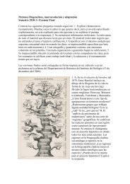
Paleobiology, 17(1), 1991, pp. 37-48A kill curve for Phanerozoic marine speciesDavid M. RaupAbstract.-A kill curve for Phanerozoic species is developed from an analysis of the stratigraphicranges of 17,621 genera, as compiled by Sepkoski. The kill curve shows that a typical species' riskof extinction varies greatly, with most time intervals being characterized by very low risk. Themean extinction rate of 0.25im.y. is thus a mixture of long periods of negligible extinction andoccasional pulses of much higher rate. Because the kill curve is merely a description of the fossilrecord, it does not speak directly to the causes of extinction. The kill curve may be useful, however,to limit choices of extinction mechanisms.David M. Raup. Department of the Geophysical Sciences, University of Chicago, Chicago, Illinois 60637Accepted: December 14, 1990Concept of the Kill CurveMany natural phenomena vary greatly inintensity and frequency. River discharge,wind velocity, and seismic activity are commonexamples. In each case, the lower intensitiesare most common and the higher intensitiesprogressively less common. Eventsof greatest magnitude are generally rare andcarry names such as "flood," "hurricane," and"earthquake." In most areas of the naturalsciences that deal with these highly variablephenomena, systems have been developed todescribe the continuum of variation and thusto locate a particular event in the continuum.This is often done by noting the average timeinterval between events of a given magnitude.Thus, the 1,000-yr flood in hydrologyis the flood level that is equaled (or exceeded)every 1,000 yr, on the average (see Raup [I9881for further discussion).The use of the average time interval betweenevents of a given magnitude is convenient,flexible, and readily applicable to anysituation for which good historical recordsexist. This approach automatically includesall the relevant information and because it isbased on a simple cumulative frequency distribution,it need not depend on any a priorimodel of the natural process. It does not evenrequire that the phenomenon have a singlecause. For example, the system is readily applicableto seismic records (Howell 1979), eventhough different earthquakes have differentgeological origins.O 1991 The Paleontological Society. All rights reserved.The average time interval between eventsof a given magr,itude is often called the returnperiod, recurrence interval, or waitingtime and is directly observable from historicalrecords as long as the record is long enoughto include events in the range of interest.Waiting time is essentially equivalent to thereciprocal of the probability of occurrence ofthe event. The 1,000-yr flood thus has a probabilityof 0.001 of occurring in any given year.Of course, the 1,000-yr flood cannot be recognizedwith only 10 yr of record, eventhough the 10 yr of record might include a1,000-yr event. Methods have been developed,especially those pioneered by Gumbel(1957), to estimate the frequency of eventshaving waiting times longer than the availablerecord, but these require extrapolationbased on a priori models.The paleontological record of extinction isideally suited to description by the approachbased on observed waiting times. The recordis long and well documented, or at least aswell documented as other records to whichthe technique is normally applied.Figure 1 shows a set of hypothetical killcurves for species. Intensity of extinction isexpressed on the ordinate as the percentageof species becoming extinct during an arbitrarilyshort time interval (10,000 yr). Frequencyis expressed on the abscissa as themean waiting time between events of a given(or greater) intensity. Thus, for the solid curvein Fig. 1, a 5% extinction occurs, on the av-0094-8373/91/1701-0003/$1.00

DAVID M. RAUPMEAN WAITING TIME(YEARS:FIGURE1. Several possible kill curves for species. For a given kill value, waiting time is the expected time betweenkilling events of equal or greater magnitude. The solid curve provides the best fit to Phanerozoic extinction data.erage, every 1 m.y., a 30% extinction occursevery 10 m.y., and a 65% extinction occursevery 100 m.y.It should be emphasized that because thewaiting times are averages with high variances,they do not imply any regular periodicityin the spacing of extinction events.Periodicity is a separate question and neednot be considered here.I present here an analysis of variation inextinction rates for species through the Phanerozoic,with the results expressed in theform of the best-fitting kill curve. The resultingkill curve is a convenient and rigorousdescription of the extinction record. It saysnothing about the causes of extinction butmay be a reasonable coordinate system forfurther exploration of causes.Species-Extinction RatesA variety of techniques and data bases havebeen used to estimate the average durationof species in the fossil record. Commonly citedresults range from 1-2 m.y. for Mesozoicammonoids (Kennedy 1977) and Siluriangraptolites (Rickards 1977) to 10 m.y. for Cenozoicbivalves (Stanley 1979) and 13 m.y, forPlanktonic foraminifera (Van Valen 1973).Valentine (1970) estimated 5-10 m.y. as anoverall average duration for all fossil marineinvertebrate species.It is widely recognized that there is substantialvariation in species duration andtherefore in its reciprocal, the species-extinctionrate. Duration varies from group to group,as indicated by the estimates just given, andin time and space. Even after normalizing forthese effects, duration is highly variable; frequencydistributions of measured durationsare strongly skewed such that most speciesin any sample have durations less than themean.Although excellent studies of species extinctionhave been published (such as thosecited above), the global data base for speciesis much too poorly sampled to allow synopticanalysis covering all groups and the entirePhanerozoic. We are obliged, therefore, towork at higher taxonomic levels and interpolateback to the species level. For this purpose,I use the July 1988 version of Sepkoski'sunpublished compendium of the ranges ofmarine genera. Permission to use these datais gratefully acknowledged.

KILL CURVE FOR MARINE SPECIES39Data BaseThe Sepkoski data base contains over 30,000genera and their stratigraphic ranges (Sepkoski1986,1989). As of July 1988, about threequartersof the genera (21,802) were assignedfirst and last appearances with precision atthe level of the stratigraphic stage or substage.Although marine vertebrates are includedin the compilation, the data base isdominated by invertebrates.As with all such compilations, the Sepkoskilist has problems of data quality ranging fromnomenclatural uncertainties to incompletesampling of stratigraphic ranges. Repeated useof the list by a variety of analysts working ondifferent problems has demonstrated, however,that the Sepkoski compilation, like itspredecessor for marine families (Sepkoski1982) is useful as a means of detecting broadpatterns. Where comparisons are possible, theSepkoski data bases produce the same patternsseen in earlier, less complete compilationsby Newel1 (1952), Simpson (1953), Miiller(1961), Schindewolf (1962), and Valentine(1969).Many of the genera in the Sepkoski list areparaphyletic and thus could not withstandclose phylogenetic scrutiny. For the purposeof this paper, the paraphyletic genera are usefulbecause they identify groups of speciesoccupying distinct regions of morphospace.The genera survive or fail in evolutionarytime by the interplay of speciation and extinctionof their constituent species. For furtherdiscussion of the paraphyly problem, seeRaup (1985) and Raup and Boyajian (1988).Outline of the AnalysisThe following steps were followed in theanalysis described in this paper.1. Using cohort survivorship techniques, abest-fit survivorship curve was constructedfor marine genera of the Phanerozoic. Thefitting process yielded, among other things,estimates of the average rates of species extinctionand origination, where species originationis confined to true speciation (as opposedto species formation by phyletictransformation) and to species serving tomaintain the parent genus (as opposed tofounding new genera).2. The null expectation of stochasticallyconstant speciation and species-extinctionrates was simulated to determine whetherpurely random variation in a homogeneousbirth-death process can explain the scatter observedabout the best-fit survivorship curve.This shows that the observed scatter (variationin rates) is dramatically greater than couldbe generated by the simple stochastic model.3. A kill curve for species was fit to thescatter in genus survivorship. The kill curveexpresses graphically the temporal variationin a typical species' risk of extinction and assuch, is analogous to risk curves constructedfor other highly variable natural phenomenasuch as river discharge, wind velocity, andseismic activity.Survivorship Analysis of Phanerozoic Genera Cohort survivorship analysis was performedusing a technique previously appliedto a primitive Phanerozoic data base (Raup1978) and used by subsequent authors formore detailed work (e.g., Foote [I9881 onCambrian and Ordovician trilobites). The followingrules were used to filter the Sepkoskidata. (1) Only genera with stratigraphic rangesknown to stage or substage were used. (2)Only genera with pre-Tertiary originationswere used in order to avoid the strong effectof the Pull of the Recent on Tertiary genera.(3)Only extinct genera were used. This, combinedwith (2), virtually eliminates the effecton survivorship of living species being falselyascribed to fossil genera. (See Raup [I9781for a fuller discussion of the reasoning behindthe filtering process.)After these eliminations, 17,621 genera wereavailable for analysis. They were segregatedinto 68 cohorts, one for each of the standardstages between the base of the Cambrian andthe top of the Cretaceous. In this scheme, agenus belongs to the cohort of a given stageif the genus' first appearance is in that stage.For analysis of these cohorts, one additionalrule was applied. (4)For purposes of the analysis,all genera in a cohort were assumed tohave originated at the midpoint of their firststage. Thus, a genus confined to a single stagewas assigned a duration equal to half that of

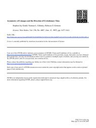
DAVID M. RAUPFIGURE2. Survivorship curves for 17,621 genera from the Sepkoski compilation. Starting at time = 0 (upper left)with full cohorts of genera (100% survival), the curves monitor the decline in number of surviving genera. Duringthe decline, new species within genera appear and become extinct. The survival time of a given genus thus dependson the balance between species origination and extinction. The solid curve passes through median survivorship.The dashed line is the theoretical curve fit to the Sepkoski data using Eq. (1).the stage. This protocol follows the practicedeveloped and justified by Van Valen (1973).The GTS 89 time scale (Harland et al. 1989)was used for dating stage boundaries.Figure 2 shows two composite survivorshipcurves: the solid curve follows the mediannumber of surviving genera, calculated at5-m.y. intervals, and the dashed curve is thebest fit using a theoretical model that assumesconstant rates of speciation and species extinction.Curve-fitting for the theoreticalcurve was done by the method described inan earlier paper (Raup 1978). Equation (3) (ofRaup 1978; equivalent to the survival versionof Eq. [A131 of Raup [1985]) was used, substitutingrates for probabilities:where S is the proportion of genera in thecohort surviving at time t, assuming that thespecies in those genera are subject to the averagerates of speciation and extinction givenby p and q, respectively.Although this equation is based on a modelwherein rates of speciation and species extinctionare stochastically constant probabilities,the equation is used here only to find theaverage rates of speciation and extinction thatbest describe the composite history of Phanerozoicgenera. Use of the equation carriesno implication of uniformity of rates.The best-fitting values of the constants forthe dashed curve in Fig. 2 are q= 0.250lm.y.and p = 0.2491m.y. Thus, on the average, onequarterof the species in a cohort of generabecome extinct every million years. The averagespecies duration is llq = 4 m.y., wellwithin the range of estimates for the Phanerozoiccited above.The 4-m.y. mean duration differs from the11 .l-m.y. estimate of Raup (1978) because theearlier study used only generalized cohortsfor large time intervals (seven pre-Jurassicsystems), thus smearing out the time scale ofgenus extinction.The average species-extinction rate of 0.251m.y. is incredibly low on human time scales:it represents 1% extinction every 40,000 yr. Ifthere were a million species in existence at agiven time, the rate would be equivalent toone species dying out every 4 yr. It must beemphasized, however, that the average rateprobably combines intervals of near-zero rateswith intervals in which rates are near-infinite(McLaren 1982). The remainder of this paperexplores this variation.

KILL CURVE FOR MARINE SPECIESTIME(YILLI5NS OF YEARS)FIGURE3. Monte Carlo simulation of survivorship for genera, based on the assumption that rates of speciation andspecies extinction are stochastically constant. Probabilities used for the simulation were taken from the dashed curveof Fig. 2.The Null Expectation: Constant Extinction.-The dashed curve in Fig. 2 predicts the decayof a cohort of genera if the species-extinctionrate is absolutely fixed at 0.25lm.y. and thewithin-genus speciation rate is fixed at 0.249.A somewhat more realistic model is one inwhich the two rates are only stochasticallyconstant, thus allowing for the vagaries ofchance. In the latter model, each decisionabout the survival or death of a species ismade by a random process with fixed probabilities.The survivorship curves for somecohorts will be steeper or shallower than expected,depending on chance. This producesscatter about the expected curve and is modeledin Fig. 3.Figure 3 was constructed by Monte Carlosimulation using the actual cohort sizes observedin the Sepkoski compilation (17,621genera with their times of origin). Each genuswas assumed to originate with a single founderspecies. At 10,000-yr intervals, each specieswas allowed to become extinct, branch to formanother species, or merely survive, withprobabilities taken from the best-fit values ofp and q in Eq. (I), above. Because the simulationcovered only decay of cohorts, it wasnot necessary to specify (or even know) therate at which new genera are formed. The10,000-yr time interval was used in the simulationbecause it is small enough to makethe probability of the co-occurrence of twoevents trivial. In all, 233,101 species were processedin the simulation.The resulting scatter of points follows thetheoretical curve of Fig. 2, as expected. Thebreadth of the scatter is a measure of theamount of stochastic variation expected underthe time-homogeneous model.Actual Variation in Extinction Rate.-WhereasFig. 3 shows what variation in survivorshipwould be like if species extinction were stochasticallyconstant, Fig. 4 shows the actualdata from the Sepkoski compilation. This isthe scatter of points that was fit statisticallyto produce the average curves in Fig. 2. Variationin extinction is dramatically greater thanwith the stochastic model. Some cohorts experiencedfar less than average extinction(higher points), whereas others sufferedhigher than expected kills (lower points).Many of the lower points can be identifiedwith well-known mass extinctions. The dataused for the plot are given in the Appendix.Comparison of the two scatter plots (Figs.3, 4) shows that extinction rates in the Phanerozoicare not stochastically constant. Theonly alternative is that the wider scatter in

DAVID M. RAUPFIGURE4. Survivorship data for 17,621 genera in 68 cohorts. Note that the scatter is much broader than that producedby the stochastic model (Fig. 3), indicating more variation in species-extinction rates than expected.Fig. 4 is due to errors in the data base. Buterrors in dating, taxonomy, and stratigraphicrange, though certainly present, are not largeenough to produce such a broad scatter. Forexample, a dating error of several millionyears in the placement of a stage boundarywould displace points in Fig. 4 but notenough, at the scale of the graph, to changethe magnitude of the scatter significantly.Only in the proximal portion (time intervalsless than about 5 m.y.) are dating errors significantand the scatter exaggerated.Figure 5B is a histogram of variation acrossthe Sepkoski data in Fig. 4, to be comparedwith that from the stochastic model (Fig. 5A).As can be seen, the histogram from the Sepkoskidata is not only much broader, but it isalso skewed.Kill CurvesThe wide scatter in Fig. 4 should come asno surprise to students of mass extinction, butthe analysis demonstrates that the variationis well beyond the expectations of the simplestochastic model. The variation must reflectan underlying probability distribution of therisk of extinction, or kill curve.Figure 1 shows several conceivable killcurves for species. Each curve indicates theprobability that extinction will exceed a giv-en level, with probability being expressed(abscissa) by its reciprocal: the waiting timebetween events of equal or greater magnitude.The kill curves in Fig. 1all use the sameequation,where WT is waiting time in units of 10,000yr and a and b are constants. The equationwas chosen because it produces the sigmoidalshape suggested by the data and because it isflexible. It has no basis in extinction theory.All kill curves in Fig. 1were chosen to yieldthe same average species extinction rate: 0.251m.y. That is, the constants, a and b, were selectedthrough a search process to producethe same mean rate. A kill curve for the stochasticmodel could be added but it wouldfall virtually on the horizontal axis and wouldbe invisible at this scale.The question now is which kill curve bestdescribes the Phanerozoic record? This willbe tackled by relating kill-curve shape to scatterin the survivorship plot (Fig. 4). As thekill curves become steeper, more of the extinctionis caused by rare events of great killingand less is caused by background extinctiontypical of shorter waiting times.Although an exact analytical solution to fittingkill curves to survivorship data may ex-

KILL CURVE FOR MARINE SPECIES43mmA. SIMULATED WITH CONSTANT EXTINCTION8. PHANEROZOIC DA-Aso0 1500,C. SIMULATED WITH KILL C3RVEHIGHERLOWERDEVIATION FROM EXPECTED SURVIVORSHIi(LOG SCALE)FIGURE5. Histograms describing variation in extinctionrate. Variation is expressed as deviation from the theoreticalsurvivorship pattern (scatter about the solid curvein Fig. 2). A, B, and C correspond to the scatters in Figs.3, 4, and 6, respectively.ist, it has not been found. Therefore, a trialand-errorsearch was conducted to find thekill curve that, in simulation, best reproducesthe scatter about the Phanerozoic survivorshipcurve.The Phanerozoic Kill CurveFigure 6 shows the results of a Monte Carlosimulation using the solid kill curve in Fig.1. A total of 295,391 species were processedin the simulation. The scatter is summarizedin Fig. 5C. This kill curve, with a = 5 and b= 10.5, replicates the Phanerozoic record (Fig.4) quite well; when other kill curves are used(dashed in Fig. I), the fit deteriorates markedly.The solid curve can thus be accepted asthe best-fit kill curve.Could the fitting of the kill curve have beeninfluenced by systematic biases in the underlyingdata? A possible source of bias is thetruncation of stratigraphic ranges caused bylack of preservation or discovery; this wouldyield an artificially steepened survivorshipcurve. Errors in taxonomic judgment couldcause bias in the same or opposite direction:oversplitting of genera makes survivorshipcurves steeper, and lumping makes them lesssteep. Unfortunately, these biases are not rigorouslymeasurable. The marked deteriorationof the fit when other kill curves are tested,noted above, suggests that the fittingprocesses are not significantly influenced bybias in the data. That is, when simulations areperformed with any of the dashed kill curvesin Fig. 1, the resulting scatter is dramaticallydifferent from that observed in the Phanerozoicdata.Because Eq. (2) for the kill curve is a continuousfunction, there can be no thresholds,or steps. The presence of thresholds cannotbe ruled out, of course, but there is no evidenceto suggest their presence. Furthermore,when histograms of extinctions have beenprepared (e.g., extinctions per stratigraphicstage), the distributions show right-skewingbut no clear bimodality or significant outliers.Only when the distributions are erroneouslyassumed to be symmetrical about the meanhas it been possible to claim that some eventsdiffer significantly from the record as a whole(see, e.g., the analysis by Raup and Sepkoski[I9821 and discussion by Stigler [1987]).As noted earlier, the 10,000-yr sampling intervalis used only for convenience becauseit is small enough to make multiple killingevents unlikely. The use of this short intervaldoes not imply that mass extinctions, such asin the late Permian or terminal Cretaceous,occurred over such a short interval, althoughthis is not precluded by the analysis.The kill curve in Fig. 1 (solid) should notbe confused with one for genera described inanother paper (Raup in press). The kill curvefor genera is purely ad hoc, whereas the speciescurve presented here was fit to actualPhanerozoic fossil data.

DAVID M. RAUPSIMU-.,4-EE? d:TL KILL CJR.EFIGURE6. Simulation of genus survivorship using the solid kill curve (Fig. 1) to determine extinction probabilities.See Fig. 5 for comparison of this scatter with those produced by actual survivorship data and by the stochasticmodel.DiscussionLet us explore some of the consequences ofthe species-kill curve. By integrating underthe curve, we can calculate the relative proportionsof background and mass extinction.Mean kill values for various segments of thekill curve are given in Table 1. Although theoverall average kill is 0.0025 per 10,000 yr,variation is large. For example, at waitingtimes less than 100,000 yr, the mean kill expectedin any 10,000-yr interval is only about0.01%. By contrast, at waiting times between10 m.y. and 100 m.y., the mean kill expectedin any 10,000-yr interval is 42%.These kill rates are well in line with experiencewith the fossil record. The mass extinctions,spaced in the 10-100 m.y. range,have species kills in the range given. TheTABLE1. Mean species kill per 10,000 yr for a series ofwaiting times, assuming a kill curve with a = 5 and b =10.5 (solid curve in Fig. 1).Waitlng tunes (pr)Mean k~llU10,OOOyr (proportion)

KILL CURVE FOR MARINE SPECIESSPECIES KILL PER E'JENT(i:)FIGURE7. Simulation of a"typicalr' Phanerozoic time interval of 600 m.y. using the kill curve to show the proportionsof total species extinction involved in small and large extinction events. Mass extinctions (tail on right) includeonly a small proportion of all species extinctions.The kill curve for Phanerozoic species saysnothing directly about the causes of extinction.It is only a description of the extinctionhistory as this history is expressed in the fossilrecord. The curve does not even speak tothe question of how many mechanisms of extinctionhave operated in the Phanerozoic.The curve does have some implications formechanisms of extinction, however. The actionof any cause or causes of extinction mustbe distributed in time in a manner compatiblewith the kill curve. This can serve to constrainour choices of mechanisms and may be usefulto eliminate some candidates. For example,various authors have proposed that Phanerozoicextinctions are dominated by a singlefactor, such as sea-level lowering, climaticcooling, or meteorite impact. These proposalscan be tested in the following manner:1. Construct a cumulative frequency curvefor the proposed mechanism; for sea-levellowering, the coordinates would be the magnitudeof sea-level drop (in short spans ofgeologic time) and the average waiting timeobserved between events of a given magnitude.2. Combine this curve with the kill curvein Fig. 1, eliminating the common variable,waiting time. This yields a curve that predictsthe average species kill for any given magnitudeof sea-level lowering (or whatevercausal factor is being considered). This stepis based on the working hypothesis-beingtested-that the proposed causal factor explainsall or most extinctions.3. Evaluate the plausibility of the new curveby inspecting specific cases where magnitude(e.g., of sea-level lowering) and extinction areboth known with reasonable accuracy.The procedure just described should workwell for any situation in which the Phanerozoichistory of the candidate mechanism iswell known. For the three examples givenabove, one needs only the chronologies ofsea-level fluctuations, temperature changes,or meteorite impacts, respectively. If one wereto postulate extinction caused by a combinationof two or more factors, the factorswould have, to be weighted and combinedand the testing would become far more complex.The kill curve also helps explain why pa-

46 DAVID M. RAUPleontologists have had such difficulty definingthe term "mass extinction." Because thekill curve is a smooth, continuous curve, oneshould not expect to find a clear demarcationbetween high- and low-intensity events; anymore than a seismologist expects to recognizea clear boundary between large and smallearthquakes, or a meteorologist expects an obviousboundary between a hurricane and asevere storm. From a procedural standpoint,the paleontologist must therefore choose betweenthe alternatives of (1) using a continuousintensity scale to describe extinction(analogous to the Richter scale for earthquakes)and (2) defining mass extinction bydrawing a totally arbitrary boundary (analogousto the convention of using windspeedof >32.7 m/s to define a hurricane).Despite the foregoing arguments, the fossilrecord does give a strong intuitive impressionof two kinds of extinction, mass extinctionand background extinction. To the extent thatthis perception is real, it is probably due tothe steepness of the middle region of the killcurve. In a typical 100-n1.y. interval of geologictime, there may be one or two largeevents, a few small but identifiable events,and hundreds or thousands of extinctions toosmall to distinguish stratigraphically. Thus,with the relatively small sample available (thePhanerozoic record), one gets an impressionof a choppier distribution of the risk of extinctionthan actually exists.AcknowledgmentsThe research described here was supportedby the National Aeronautics and Space Administration(USA) under grant NAG W-1527.I thank J. J. Sepkoski, Jr. and David Jablonskifor many fruitful discussions. Special thanksare due J. J. Sepkoski, Jr. for making availablehis unpublished compilation of the ranges ofPhanerozoic marine genera.Literature CitedFOOTE,M. J. 1988. Survivorship analysis of Cambrian and Ordov~ciantrilobites. Paleobiology 14:258-271GUMBEL, E. J. 1957. Statistics of Extremes. Columbia UniversityPress; New York.HARLAND,hT. B., R. L. ARMSTRONG, A. V. COX, L. 5. CRAIG, A. GSMITH,AND D. G. SMITH. 1989. A Geologic Time Scale 1989.Cambridge University Press; Cambridge.HOWELL, B. F ,JR. 1979 Earthquake risk in eastern Pennsylvania.Earth and Mineral Sciences 48.63-64 KENNEDY, W J 1977. Ammonite evolution. Pp. 251-304 In Hallam,A. (ed.), Patterns of Evolution. Elsev~er Scientihc PublishingCompany, Amsterdam.MCLAREN,D. J. 1982. Frasnian-Famennian extinctions. GeologicalSociety of America Special Paper 190:477-484MULLER,A. H. 1961. Grossablaufe der Stammesgeschichte. GustavFischer Verlag; Jena.NEWELL, N. D 1952 Periodlclty In invertebrate evolution. Journalof Paleontology 26:371-385.RAuP, D. M. 1978. Cohort analysis of generlc survlvorship. Paleobiology4.1-15.RAUP, D. M. 1979. Size of the Permo-Triassic bottleneck and itsevolutionary implications. Science 206:217-218.RAUP, D. M. 1985. Mathematical models of cladogenesis. Paleobiology11 :42-52.RAUP,D. M. 1988. Changing views of natural catastrophe. Pp.5-77. In Adler, M. J. (ed.), Great Ideas Today (1988). EncyclopaediaBritannica; Chicago.RAuP, D. M. In Press. Impact as a general cause of extinction:a feasibility test. Geological Society of America Special Paper24i.RAUP, D. M., AND G E. BOYAJIAN. 1988. Patterns of generlcextinction in the fossil record. Paleobiology 14:109-125.RAUP,D. M., AND J. J. SEPKOSKI, JR. 1982. Mass extinctions inthe marine fossil record. Science 215:1501-1503.RICKARDS, R. B. 1977 Patterns of evolution in the graptolites.Pp. 333-358. irr Hallam, A. (ed.), Patterns of Evolution. ElsevierScientific Publishing Company; Amsterdam.SCHINDEWOLF, 0.H. 1962. Neokatastrophismus? Deutsche GeologischesGesellschafte Zeitschrifte 114:430-445.SEPKOSKI, J.J., JR. 1982. A compendium of fossil marine families.Milwaukee Public Museum Contributions in Biology and Geology51.SEPKOSKI, J. J., JR. 1986. Phanerozoic overview of mass extinction.Pp. 277-295. In Raup, D. M., and D. Jablonski (eds.), Patternsand Processes in the History of Life. Springer; Berlin.SEPKOSKI, J. J., JR. 1989. Periodicity in extinction and the problemof catastrophism in the history of life. Journal of the GeologicalSociety of London 146:7-19.SIMPSON, G. G. 1953. The Major Features of Evolution. ColumbiaUniversity Press; New York.STANLEY, S. M. 1979 Macroevolution. Pattern and Process. W.H. Freeman and Company; San FranciscoSTIGLER, S M. 1987. Testing hypotheses or fitting models? Pp.147-159. In Nitecki, M. H., and A. Hoffman (eds.), NeutralModels in Biology Oxford University Press; Oxford.VALENTINE, J W, 1969 Patterns of taxonomic and ecologic structureof the shelf benthos during Phanerozoic time. Palaeontology12:684-709.VALENTINE, J. W. 1970 How many marine invertebrate fossilspecies? Journal of Paleontology 44:410-415.VALENTINE, J. W., T. C. FOIN, AND D. PEART. 1978. A provincialmodel of Phanerozoic marine diversity. Paleobiology 4:55-66.VAN VALEN, L. 1973. A new evolutionary law. EvolutionaryTheory 1:l-30Appelzdix: Data for Survivorsh~p Arralysis David M. Raup and J. John Sepkoski*Table A1 provides the raw data for the cohort analysis describedin this paper. The data were assembled by D.M.R. fromstratigraphic ranges compiled by J.J.S.A total of 17,621 genera' Department of the Geophys~cal Sc~ences, Unlvers~ty of Chlcago, Chicago,Ill~no~s 60637

TABLEAl. Survivorship data used in this analysis. Numbers of surviving genera are monitored at stage boundaries until the cohortis completely extinct or until 55 m.y, has passed (from the mid-point of the initial stage).Stage Age at base Ma Genera In onglnal cohort Number of genera survlvlng to base of each succeed~ng stageN-DaTommAtdaBotolMidmMiduMidDresFranTrepTremArenLlviLldeCaraAshgLdovWen1LudlPridGediSiegEmsiEifeGiveFrasFameTourViseSerpBashMoscStepAsseSakmLeonGuadDjhuDoraInduOlenAnisLadiCarnNoriHettSinePlieToarAaleBajoBathCallOxfoKimmTithBerrBalaHautBarrAptiAlbiCenoTuroConiSantCampMaes162 313 - 262 17,621 aenera ( 136321 61 33 21 18 14 10 7 6 6 100 41 32 23 11 9 7 7 69392286555 512662222 661577765 77932 70 30 21 10 6 5 4 79 29 11 6 2 1 46 14 6 5 5 113 65 53 44 283 196 157 108 50 39 230 177 114 58 49 40 270 157 62 51 39 355 143 107 78 62 56 99 71 51 37 31 24 24 267 189 124 109 92 85 68 48 234 144 113 86 74 64 46 32 135 94 67 58 35 26 21 13 10 61 36 31 28 22 15 8 3 195 146 99 65 42 28 23 18 210 114 58 35 15 9 7 226 128 61 21 15 13 192 99 49 29 23 19 110 56 34 28 21 89 35 24 18 15 105 71 43 27 21 281 142 103 86 71 257 133 103 78 63 86 66 44 33 30 124 80 44 42 36 134 68 59 46 34 75 68 50 36 15 5 2 2 81643911321111 120691653111 11 155 53 23 11 10 9 9 9 5 3 53 31 19 14 13 13 13 10 4 4 27887666333 4 4 3 3 3 3 16 12 12 11 10 5 5 5 34 27 23 20 9 9 9 124 93 63 28 26 24 20 126 63 29 28 26 22 110 40 40 39 31 27 58 54 52 44 41 40 35 32 54 48 34 29 28 25 23 21 19 17 95 65 43 42 32 30 28 27 26 17 76 52 49 41 40 37 34 32 22 22 66 57 46 43 40 32 29 15 13 13 12 58 36 34 28 24 22 18 17 17 13 13 113 90 69 59 46 34 32 29 27 24 112 75 70 65 48 46 44 41 40 32 82 54 47 27 24 20 20 19 18 121 70 42 39 33 28 25 18 71 36 33 27 26 22 18 75 60 42 37 33 23 20 43 31 24 21 14 12 8 8 75 61 52 39 32 20 20 19 17 63 43 28 24 17 16 15 14 87 53 38 27 20 17 16 16 107 73 51 45 43 39 33 9 167 96 75 72 69 61 18 12 10 10 180 134 127 120 91 30 15 11 9 113 95 88 74 15 11 6 4 4 4 93 69 53 12 10 8 7 5 4 105 61 13 8 6 6 4 2 190 38 24 15 10 9 4 3 48 32 18 15 9 4 4 3 3 extant taxa excluded)

DAVID M. RAUPare distributed among 68 pre-Tertiary cohorts, one for each stratigraphicstage. For each cohort, the table gives the number ofgenera having first appearances in the named stage, followed bythe number of genera still surviving at the base of each succeedingstage, continuing until all genera are extinct or until 55m.y. have passed (beyond the midpoint of the initial stage). Forexample, 13 of the genera in the first cohort are found in theTommotian (or younger stages) and thus must have existed atthe start of Tommotian time (570 Ma); 6 of these are found inthe Atdabanian (or younger stages) and must have existed at thestart of the Atdabanian (560 Ma), and so on.The 513 tabulated survivorship values are plotted (as proportionsof original cohort size) in Fig. 4. Given these data, thesurvivorship results and the fitting of the k~ll curve can be reproduced.Abbreviations of stage names are those used by Sepkoski (1982).Geologic ages of stage bases are from the GTS 89 time scale(Harland et al. 1989), with the ages for the upper Middle Cambrian(uMid) and Trempealeauan (Trem) interpolated. The Tertiarystages used for monitoring the late Cretaceous cohorts are:Danian (65 Ma at base), Thanetian (60.5), Lower Eocene (56.5),Middle Eocene (50), Upper Eocene (38.6), Lower Oligocene (35.4),Upper Oligocene (29.3), Lower Miocene (23 3), and Middle Miocene(16.3).Readers wishing to use these data for other purposes, such ascomputing diversity curves or stage-level extinction rates, shouldbe cautioned that the tabulated cohorts do not include extantgenera. As noted in the text, the extant genera were eliminatedto minimize the Pull of the Recent.