Cross-Asset Speculation in Stock Markets∗ - Econometrics at Illinois ...
Cross-Asset Speculation in Stock Markets∗ - Econometrics at Illinois ...
Cross-Asset Speculation in Stock Markets∗ - Econometrics at Illinois ...

You also want an ePaper? Increase the reach of your titles
YUMPU automatically turns print PDFs into web optimized ePapers that Google loves.
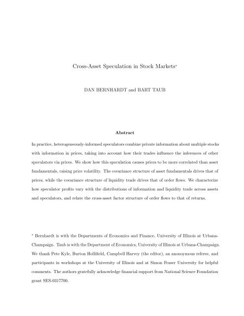
<strong>Cross</strong>-<strong>Asset</strong> <strong>Specul<strong>at</strong>ion</strong> <strong>in</strong> <strong>Stock</strong> Markets ∗DAN BERNHARDT and BART TAUBAbstractIn practice, heterogeneously-<strong>in</strong>formed specul<strong>at</strong>ors comb<strong>in</strong>e priv<strong>at</strong>e <strong>in</strong>form<strong>at</strong>ion about multiple stockswith <strong>in</strong>form<strong>at</strong>ion <strong>in</strong> prices, tak<strong>in</strong>g <strong>in</strong>to account how their trades <strong>in</strong>fluence the <strong>in</strong>ferences of otherspecul<strong>at</strong>ors via prices. We show how this specul<strong>at</strong>ion causes prices to be more correl<strong>at</strong>ed than assetfundamentals, rais<strong>in</strong>g price vol<strong>at</strong>ility. The covariance structure of asset fundamentals drives th<strong>at</strong> ofprices, while the covariance structure of liquidity trade drives th<strong>at</strong> of order flows. We characterizehow specul<strong>at</strong>or profits vary with the distributions of <strong>in</strong>form<strong>at</strong>ion and liquidity trade across assetsand specul<strong>at</strong>ors, and rel<strong>at</strong>e the cross-asset factor structure of order flows to th<strong>at</strong> of returns.∗ Bernhardt is with the Departments of Economics and F<strong>in</strong>ance, University of Ill<strong>in</strong>ois <strong>at</strong> Urbana-Champaign. Taub is with the Department of Economics, University of Ill<strong>in</strong>ois <strong>at</strong> Urbana-Champaign.We thank Pete Kyle, Burton Hollifield, Campbell Harvey (the editor), an anonoymous referee, andparticipants <strong>in</strong> workshops <strong>at</strong> the University of Ill<strong>in</strong>ois and <strong>at</strong> Simon Fraser University for helpfulcomments. The authors gr<strong>at</strong>efully acknowledge f<strong>in</strong>ancial support from N<strong>at</strong>ional Science Found<strong>at</strong>iongrant SES-0317700.
<strong>Stock</strong> markets are characterized by many stocks and many traders. Specul<strong>at</strong>ors, especially <strong>in</strong>stitutionaltraders, often <strong>in</strong>teract str<strong>at</strong>egically <strong>in</strong> many stocks simultaneously. When asset values arecorrel<strong>at</strong>ed, priv<strong>at</strong>e <strong>in</strong>form<strong>at</strong>ion about one stock may well provide a specul<strong>at</strong>or <strong>in</strong>form<strong>at</strong>ion aboutother stocks th<strong>at</strong> he will <strong>in</strong>corpor<strong>at</strong>e <strong>in</strong> his trad<strong>in</strong>g. For example, a specul<strong>at</strong>or with priv<strong>at</strong>e <strong>in</strong>form<strong>at</strong>ionabout a new drug from Merck th<strong>at</strong> affects the value of Glaxo Smith Kl<strong>in</strong>e may trade both stocks.But str<strong>at</strong>egic <strong>in</strong>teractions are far richer than just this observ<strong>at</strong>ion suggests. In practice, specul<strong>at</strong>orsalso observe prices and use th<strong>at</strong> <strong>in</strong>form<strong>at</strong>ion when trad<strong>in</strong>g. Concretely, traders may use<strong>in</strong>form<strong>at</strong>ion <strong>in</strong> the price of Glaxo to adjust trades of Merck. Specul<strong>at</strong>ors also understand th<strong>at</strong> theirtrades convey <strong>in</strong>form<strong>at</strong>ion to others via their impacts on prices; and th<strong>at</strong> prices reflect <strong>in</strong>form<strong>at</strong>ionof other specul<strong>at</strong>ors th<strong>at</strong> they, themselves, can use.The contribution of this paper is to characterize equilibrium outcomes <strong>in</strong> this sett<strong>in</strong>g. To dothis, we first solve for how specul<strong>at</strong>ors comb<strong>in</strong>e priv<strong>at</strong>e <strong>in</strong>form<strong>at</strong>ion about different assets with thepublic <strong>in</strong>form<strong>at</strong>ion <strong>in</strong> prices to determ<strong>in</strong>e how much of each stock to trade. We then derive explicitanalytical characteriz<strong>at</strong>ions of the correl<strong>at</strong>ion structure of prices and order flows, determ<strong>in</strong><strong>in</strong>g bothhow are they driven by the correl<strong>at</strong>ion structure of asset fundamentals and liquidity trade, and howthey are affected by the observability of prices; <strong>in</strong> addition, we quantify the l<strong>in</strong>ks between the factorstructures of order flows and prices. F<strong>in</strong>ally, we document numerically how trad<strong>in</strong>g str<strong>at</strong>egies andprofits vary with the distributions of <strong>in</strong>form<strong>at</strong>ion and liquidity trade across assets and specul<strong>at</strong>ors.The central studies of multi-asset stock markets are Adm<strong>at</strong>i (1985) and Caballe and Krishnan(1994). Each of these papers simplifies the str<strong>at</strong>egic sett<strong>in</strong>g along one dimension to obta<strong>in</strong> answersabout other dimensions. Adm<strong>at</strong>i develops a multi-asset, noisy r<strong>at</strong>ional expect<strong>at</strong>ions model with acont<strong>in</strong>uum of agents. Her model has the fe<strong>at</strong>ure th<strong>at</strong> agents condition trades on both their priv<strong>at</strong>esignals and stock prices. However, the cont<strong>in</strong>uum of agents precludes <strong>in</strong>dividual str<strong>at</strong>egic behavior—the <strong>in</strong>form<strong>at</strong>ionally-small agents ignore the price impact of their trades and do not have to accountfor how their trades affect <strong>in</strong>form<strong>at</strong>ion release. But, <strong>in</strong> practice, <strong>in</strong>formed agents for a given stockare few <strong>in</strong> number. Those few specul<strong>at</strong>ors are typically <strong>in</strong>stitutional traders who understand th<strong>at</strong>their significant trad<strong>in</strong>g has price impacts th<strong>at</strong> they should and do anticip<strong>at</strong>e and <strong>in</strong>ternalize. Torealistically model trad<strong>in</strong>g, it is important to account for such str<strong>at</strong>egic <strong>in</strong>formed trade.Caballe and Krishnan (1994) develop a st<strong>at</strong>ic multi-asset formul<strong>at</strong>ion of the competitive dealer-1
ship model of Kyle (1985) and Adm<strong>at</strong>i and Pfleiderer (1988): specul<strong>at</strong>ors <strong>in</strong>ternalize the price impactsof their trades, but do not see prices. Hence, as <strong>in</strong> Adm<strong>at</strong>i (1985), specul<strong>at</strong>ors need not worryabout the <strong>in</strong>form<strong>at</strong>ion their trades convey to other specul<strong>at</strong>ors. But, <strong>in</strong> practice, specul<strong>at</strong>ors use <strong>in</strong>form<strong>at</strong>ion<strong>in</strong> stock prices when trad<strong>in</strong>g, and they worry about <strong>in</strong>form<strong>at</strong>ion dissem<strong>in</strong><strong>at</strong>ion via prices.Our model melds these two models, cre<strong>at</strong><strong>in</strong>g a str<strong>at</strong>egic analogue of Adm<strong>at</strong>i’s noisy REE model,along the l<strong>in</strong>es of Kyle (1989). 1 As <strong>in</strong> Adm<strong>at</strong>i, risk-neutral specul<strong>at</strong>ors comb<strong>in</strong>e priv<strong>at</strong>e <strong>in</strong>form<strong>at</strong>ionabout various stocks with the <strong>in</strong>form<strong>at</strong>ion <strong>in</strong> prices to determ<strong>in</strong>e how much of each stock to trade.As <strong>in</strong> Caballe and Krishnan, specul<strong>at</strong>ors <strong>in</strong>ternalize how trades <strong>in</strong>fluence prices. In dynamic stockmarkets, specul<strong>at</strong>ors use <strong>in</strong>form<strong>at</strong>ion <strong>in</strong> exist<strong>in</strong>g prices when determ<strong>in</strong><strong>in</strong>g trades, and str<strong>at</strong>egicallyaccount for how, via prices, their trades <strong>in</strong>fluence the <strong>in</strong>ferences of other specul<strong>at</strong>ors, and hence thetrades of other specul<strong>at</strong>ors. Comb<strong>in</strong><strong>in</strong>g observable prices with str<strong>at</strong>egic specul<strong>at</strong>ors lets us capturethis key fe<strong>at</strong>ure of real world markets <strong>in</strong> a tractable st<strong>at</strong>ic sett<strong>in</strong>g. In particular, a specul<strong>at</strong>or <strong>in</strong>our model must account for how, via prices, his trades <strong>in</strong>fluences those of other specul<strong>at</strong>ors.We first derive the form of equilibrium str<strong>at</strong>egies. We prove th<strong>at</strong> str<strong>at</strong>egies have a forecast errorstructure: from their direct trades on priv<strong>at</strong>e signals, traders subtract the projections onto netorder flows, so th<strong>at</strong> a specul<strong>at</strong>or’s net trades correspond to the errors <strong>in</strong> market maker forecasts ofhis direct trades. The economics underly<strong>in</strong>g this result is th<strong>at</strong> a specul<strong>at</strong>or’s relevant priv<strong>at</strong>e <strong>in</strong>form<strong>at</strong>ionconsists of the differences between wh<strong>at</strong> his signals are and wh<strong>at</strong> market makers perceivethose signals to be.We then prove th<strong>at</strong> there is a unique l<strong>in</strong>ear equlibrium. Establish<strong>in</strong>g the existence of an equilibriumis a formidable task due to the m<strong>at</strong>rix structure <strong>in</strong>herent <strong>in</strong> multi-asset sett<strong>in</strong>gs. Withobservable prices and non-str<strong>at</strong>egic traders, Adm<strong>at</strong>i (1985) sets out (p. 633) the technical difficultiesfor why the methods used by Hellwig (1980) to prove existence for a s<strong>in</strong>gle asset do not extend.Indeed, Adm<strong>at</strong>i does not prove existence. Str<strong>at</strong>egic, <strong>in</strong>form<strong>at</strong>ionally-large specul<strong>at</strong>ors present furtherchallenges: we must resolve the forecast<strong>in</strong>g-the-forecasts-of-others issues th<strong>at</strong> arise <strong>in</strong> thismulti-asset str<strong>at</strong>egic sett<strong>in</strong>g when specul<strong>at</strong>ors use priv<strong>at</strong>e <strong>in</strong>form<strong>at</strong>ion to filter the <strong>in</strong>form<strong>at</strong>ion <strong>in</strong>prices (see Townsend 1985, Pearlman and Sargent 2005, or Mal<strong>in</strong>ova and Smith 2003).To prove existence, we set up an iter<strong>at</strong>ive best-response mapp<strong>in</strong>g. Given an <strong>in</strong>itial conjectureabout trad<strong>in</strong>g str<strong>at</strong>egies—a conjectured m<strong>at</strong>rix of trad<strong>in</strong>g <strong>in</strong>tensities—we compute the associ<strong>at</strong>ed2
l<strong>at</strong>ors see prices, they use Merck signals to trade Glaxo because they can subtract from theirtrades on signals the projections onto prices, reduc<strong>in</strong>g the <strong>in</strong>form<strong>at</strong>ion th<strong>at</strong> market makerscan extract from each order flow, thereby mitig<strong>at</strong><strong>in</strong>g the total price impacts of their trades.• We derive how the factor structure of order flow is rel<strong>at</strong>ed to th<strong>at</strong> of prices. Hasbrouckand Seppi (2001) apply a pr<strong>in</strong>cipal component decomposition of cross-asset order flows andreturns, and f<strong>in</strong>d th<strong>at</strong> commonality <strong>in</strong> order flows expla<strong>in</strong>s roughly two-thirds of the commonality<strong>in</strong> returns. We carry out a similar decomposition <strong>in</strong> our model. We f<strong>in</strong>d th<strong>at</strong> amoder<strong>at</strong>e cross-asset correl<strong>at</strong>ion <strong>in</strong> asset value fundamentals plus a slight positive correl<strong>at</strong>ion<strong>in</strong> liquidity trade across assets can quantit<strong>at</strong>ively m<strong>at</strong>ch their empirical f<strong>in</strong>d<strong>in</strong>g. 3 The primitiveparameters th<strong>at</strong> we identify—the correl<strong>at</strong>ions <strong>in</strong> <strong>in</strong>form<strong>at</strong>ion and liquidity trade—thusprovide a theoretical underp<strong>in</strong>n<strong>in</strong>g to Hasbrouck and Seppi’s purely empirical analysis.We conclude by provid<strong>in</strong>g the first quantit<strong>at</strong>ive characteriz<strong>at</strong>ions of equilibrium outcomes <strong>in</strong>multi-asset str<strong>at</strong>egic sett<strong>in</strong>gs for both symmetric and asymmetric environments.• We f<strong>in</strong>d th<strong>at</strong> observable prices drive expected specul<strong>at</strong>or profits down sharply, especiallywhen there are more specul<strong>at</strong>ors. Underly<strong>in</strong>g this result is the <strong>in</strong>form<strong>at</strong>ion exchange throughprices, which <strong>in</strong>duces specul<strong>at</strong>ors to trade more aggressively. In particular, each specul<strong>at</strong>or<strong>in</strong>ternalizes the fact th<strong>at</strong> as he <strong>in</strong>creases an order, other specul<strong>at</strong>ors see the price impacts andreduce their orders.• We f<strong>in</strong>d th<strong>at</strong> the impact of the division of <strong>in</strong>form<strong>at</strong>ion between specul<strong>at</strong>ors is very differentfrom the impact of the division of <strong>in</strong>form<strong>at</strong>ion or liquidity trade across assets. Total specul<strong>at</strong>orprofits are very sensitive to the division of <strong>in</strong>form<strong>at</strong>ion between specul<strong>at</strong>ors, fall<strong>in</strong>gsharply when <strong>in</strong>form<strong>at</strong>ion is more evenly divided and prices are observable. In stark contrast,divisions of <strong>in</strong>form<strong>at</strong>ion or liquidity trade across assets have only second-order effects on totalspecul<strong>at</strong>or profits. However, this profit irrelevance result masks the complic<strong>at</strong>ed ways <strong>in</strong>which asymmetries across assets <strong>in</strong>teract with the market structure to <strong>in</strong>fluence how specul<strong>at</strong>orstrade, and how equilibrium prices weight order flows <strong>in</strong> each market. For example,specul<strong>at</strong>ors may trade aga<strong>in</strong>st their cross-asset <strong>in</strong>form<strong>at</strong>ion <strong>in</strong> a rel<strong>at</strong>ively illiquid market.4
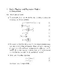
We next set out the model and analyze a specul<strong>at</strong>or’s optimiz<strong>at</strong>ion problem. We then specializeto a symmetric sett<strong>in</strong>g to obta<strong>in</strong> analytical results. Section 4 offers numerical characteriz<strong>at</strong>ions,show<strong>in</strong>g how asymmetries affect outcomes. A conclusion follows. All proofs are <strong>in</strong> the appendix.IThe modelIn our multi-asset model of specul<strong>at</strong>ive trade <strong>in</strong> a stock market, specul<strong>at</strong>ors are str<strong>at</strong>egic and <strong>in</strong>ternalizehow their trades affect prices, and hence the <strong>in</strong>ferences and trades of other specul<strong>at</strong>ors.N risk-neutral <strong>in</strong>formed specul<strong>at</strong>ors and exogenous noise traders trade claims to M assets. Pricesare set by risk-neutral, competitive, un<strong>in</strong>formed market makers.We denote the vector of asset values by v ′ = (v 1 ,...,v M ). We consider a very general formul<strong>at</strong>ion<strong>in</strong> which asset values are l<strong>in</strong>ear functions of K underly<strong>in</strong>g fundamentals, e ′ = (e 1 ,...,e K ).These K fundamentals are jo<strong>in</strong>tly normally distributed with means th<strong>at</strong> we normalize to zero andan arbitrary variance-covariance m<strong>at</strong>rix, Σ e . The value of asset j is given byv j = v j1 e 1 + v j2 e 2 + ... + v jK e K .We can write the vector of asset values as v = V e, where V is the M × K m<strong>at</strong>rix,⎛⎞v 11 v 12 ... v 1Kv 21 v 22 ... v 2K..⎜ . . .. . ⎟⎝⎠v M1 v M2 ... v MKWe allow for the possibility th<strong>at</strong> each specul<strong>at</strong>or has access to many sources of priv<strong>at</strong>e <strong>in</strong>form<strong>at</strong>ionabout asset values. Specifically, we let specul<strong>at</strong>or i see a vector of signals about the valuefundamentals,s i = A i e, where A i is an L i × K m<strong>at</strong>rix,⎛ ⎞ ⎛s i 1 A i 11 A i 12 ... A i 1Ks i 2A i 21 A i 22 ... A i 2K=.⎜ . ⎟ ⎜ . . .. .⎝ ⎠ ⎝s i L iA i L i 1 A i L i 2 ... A i L i K⎞⎛⎟⎜⎠⎝⎞e 1e 2.. ⎟⎠e KExample: One specul<strong>at</strong>or sees an asset’s value. There are M assets, N = M specul<strong>at</strong>ors,and K = M fundamentals. The value of asset j is v j = e j , i.e., V is the M × M identity m<strong>at</strong>rix.5
Only specul<strong>at</strong>or i sees v i = e i , i.e., s i i = e i and s i j = 0, j ≠ i. The Ai m<strong>at</strong>rix captur<strong>in</strong>g specul<strong>at</strong>ori’s <strong>in</strong>form<strong>at</strong>ion is an M × M m<strong>at</strong>rix, which has only zero entries save for A i ii , which is one.Example: Each specul<strong>at</strong>or receives one signal for each asset. There are M assets, N specul<strong>at</strong>ors,and K = MN fundamentals. The value of asset j is v j = e (j−1)N+1 +...+e (j−1)N+i +...+e jN .Thus, V is an M × MN m<strong>at</strong>rix, where the j th row of V captures the value of asset j, so it hasv j,(j−1)N+i = 1, for i = 1,... ,N, and zeros elsewhere. Specul<strong>at</strong>or i sees s i j = e (j−1)N+i for assetj = 1,... M. Then A i is an M × MN m<strong>at</strong>rix, where j th row of the A i m<strong>at</strong>rix captures specul<strong>at</strong>ori’s <strong>in</strong>form<strong>at</strong>ion about asset j: it has A i j,(j−1)N+i= 1, and zeros elsewhere.In addition to his signals s i , specul<strong>at</strong>or i knows the prices <strong>at</strong> which orders for each asset willbe executed. Th<strong>at</strong> is, our economy is a noisy r<strong>at</strong>ional expect<strong>at</strong>ions economy <strong>in</strong> which agents arestr<strong>at</strong>egic and <strong>in</strong>ternalize how their trades affect prices and the <strong>in</strong>form<strong>at</strong>ion content of prices. Itis <strong>in</strong> this sense th<strong>at</strong> our model extends and melds the models of Adm<strong>at</strong>i (1985) and Caballe andKrishnan (1993), allow<strong>in</strong>g us to capture key aspects of a dynamic market <strong>in</strong> a simpler st<strong>at</strong>ic sett<strong>in</strong>g.Let x i j be specul<strong>at</strong>or i’s order for asset j, let xi′ = (x i 1 ,xi 2 ,... ,xi M) be the vector of his orders,and let X ′ = (X 1 ,X 2 ,... ,X M ) ′ = ( ∑ Ni=1 xi 1 ,∑ Ni=1 xi 2 ,...,∑ Ni=1 xi M) be the vector of net order flowsacross assets from specul<strong>at</strong>ors. In addition to trade from specul<strong>at</strong>ors, there is exogenous liquiditytrade of asset j of u j . We let u ′ = (u 1 ,u 2 ,... ,u M ) be the vector of liquidity trades. Liquiditytrade is distributed <strong>in</strong>dependently of the value fundamentals, and hence of specul<strong>at</strong>or signals. Weallow for a general correl<strong>at</strong>ion structure <strong>in</strong> liquidity trade across assets, assum<strong>in</strong>g only th<strong>at</strong> liquiditytrade is jo<strong>in</strong>tly normally distributed with zero mean and variance-covariance m<strong>at</strong>rix Σ u .Markets are cleared by competitive market makers who use the trad<strong>in</strong>g activity throughout theentire stock market when sett<strong>in</strong>g prices. In particular, a market maker observes the net order flowfor his asset, and the prices of other assets. Equivalently, with l<strong>in</strong>ear pric<strong>in</strong>g, market makers seethe vector of net order flows for all assets, (X + u) ′ = (X 1 + u 1 ,X 2 + u 2 ,... X m + u m ). Marketmakers set the price of each asset equal to its expected value given the vector of net order flows,i.e., p j = E[v j |(X + u) ′ ]: competition drives market-maker expected profits from fill<strong>in</strong>g each orderdown to zero. At the period’s end, assets are liquid<strong>at</strong>ed and trad<strong>in</strong>g profits are realized.We focus on equilibria <strong>in</strong> which specul<strong>at</strong>ors adopt trad<strong>in</strong>g str<strong>at</strong>egies th<strong>at</strong> are l<strong>in</strong>ear functions ofboth their priv<strong>at</strong>e signals and net order flows, and market makers set prices th<strong>at</strong> are l<strong>in</strong>ear functions6
of net order flows. Specifically, we conjecture th<strong>at</strong> specul<strong>at</strong>or i’s order for asset j takes the form,x i j = b i j1s i 1 + b i j2s i 2 + ... + b i jL is i jL i+ B i j1(X 1 + u 1 ) + B i j2(X 2 + u 2 ) + ... + B i jM(X M + u M ).Hence, the vector of specul<strong>at</strong>or i’s orders is x i = b i s i + B i (X + u), i.e.,⎛ ⎞ ⎛⎞ ⎛ ⎞ ⎛x i 1 b i 11 b i 12 ... b i 1L is 1 B 11 i B12 i ... B1Mi x i 2b i 21 b i 22 ... b i 2L =is 2B21 i B22 i ... B2Mi . +⎜ . ⎟ ⎜ . . .. . . ⎟ ⎜ . ⎟ ⎜ . . .. .⎝ ⎠ ⎝⎠ ⎝ ⎠ ⎝x i Mb i M1b i M2... b i ML is Li BM1 i BM2 i ... BMMi⎞⎛⎟⎜⎠⎝⎞X 1 + u 1X 2 + u 2.. ⎟⎠X M + u MThus, b i represents i’s trad<strong>in</strong>g <strong>in</strong>tensities on his signals, and B i represents i’s trad<strong>in</strong>g <strong>in</strong>tensitieson the net order flows th<strong>at</strong> he sees. The conjecture th<strong>at</strong> pric<strong>in</strong>g is a l<strong>in</strong>ear function of net orderflows implies th<strong>at</strong> p = λ(X + u), where the pric<strong>in</strong>g m<strong>at</strong>rix λ is an M × M <strong>in</strong>vertible m<strong>at</strong>rix th<strong>at</strong>aggreg<strong>at</strong>es <strong>in</strong>form<strong>at</strong>ion from the order flows of all assets to determ<strong>in</strong>e prices, i.e.,⎛ ⎞ ⎛⎞⎛⎞p 1 λ 11 λ 12 ... λ 1M X 1 + u 1p 2λ 21 λ 22 ... λ 2MX 2 + u 2=..⎜ . ⎟ ⎜ . . .. . ⎟⎜. ⎟⎝ ⎠ ⎝⎠⎝⎠p M λ M1 λ M2 ... λ MM X M + u MThe extent to which a market maker uses <strong>in</strong>form<strong>at</strong>ion from other stocks to price a particular stock,and not just a stock’s own order flow, is captured by the non-diagonal elements of λ. Because thepric<strong>in</strong>g m<strong>at</strong>rix λ is <strong>in</strong>vertible, observ<strong>in</strong>g prices is equivalent to observ<strong>in</strong>g net order flows.Equilibrium. In a l<strong>in</strong>ear equilibrium, specul<strong>at</strong>ors maximize expected trad<strong>in</strong>g profits given correctconjectures, net order flows are consistent with specul<strong>at</strong>or optimiz<strong>at</strong>ion, and market makers earnzero expected profits from fill<strong>in</strong>g each order given the vector of net order flows.Specul<strong>at</strong>or’s Optimiz<strong>at</strong>ion Problem. Specul<strong>at</strong>or i seeks to maximize expected trad<strong>in</strong>g profitsgiven his signals s i and the net order flows X + u, solv<strong>in</strong>g⎡max E [ (v − p)) ′ x i |s i ,X + u ] ( ( N ′⎤∑= max E ⎣ v − λ x k + u))x i |s i ,X + u⎦ . (1)x ix iTo solve for specul<strong>at</strong>or i’s best response to the conjectured l<strong>in</strong>ear trad<strong>in</strong>g str<strong>at</strong>egies of the otherspecul<strong>at</strong>ors and the l<strong>in</strong>ear pric<strong>in</strong>g, we first rewrite the vector of net order flows from i’s perspective,X + u = x i + ∑ k≠ik=1()b k s k + B k (X + u) + u. (2)7
Def<strong>in</strong><strong>in</strong>g q i ≡ (I − ∑ k≠i Bk ) −1 , we solve equ<strong>at</strong>ion (2) forX + u = q i( x i + ∑ k≠ib k s k + u ) . (3)Specul<strong>at</strong>or i understands and <strong>in</strong>ternalizes how his orders affect the trades of other specul<strong>at</strong>orsthrough price via q i . Substitut<strong>in</strong>g for X + u <strong>in</strong>to specul<strong>at</strong>or i’s objective yields,⎡⎛⎛⎞⎞max E ⎣⎝v − λq i ⎝x i + ∑ ′ ⎤b k s k + u⎠⎠x i |s i ,X + u⎦ . (4)x ik≠iThe associ<strong>at</strong>ed first-order condition with respect to x i is∣[∣∣∣∣ ]0 = E (v − λ(X + u)) ′ − q i′ λ ′ x i s i ,X + u . (5)Proposition 1 describes the forecast-error structure of a specul<strong>at</strong>or’s orders.Proposition 1 Specul<strong>at</strong>or i’s vector of orders, x i , is a l<strong>in</strong>ear function of the forecast errors of histrades on his priv<strong>at</strong>e signals.Proposition 1 reflects th<strong>at</strong> a specul<strong>at</strong>or’s relevant priv<strong>at</strong>e <strong>in</strong>form<strong>at</strong>ion consists of the differencesbetween wh<strong>at</strong> his signals s i are, and wh<strong>at</strong> the market maker perceives them to be—i.e., the errors<strong>in</strong> the market maker’s forecasts of his signals, s i −E[s i |X +u]. Accord<strong>in</strong>gly, the vector of specul<strong>at</strong>ori’s net orders, x i , is a l<strong>in</strong>ear function of these forecast errors. Th<strong>at</strong> is, B i is a m<strong>at</strong>rix of projectioncoefficients of trad<strong>in</strong>g <strong>in</strong>tensities on priv<strong>at</strong>e signals onto net order flows: from their direct tradeson priv<strong>at</strong>e signals, traders subtract the projections of these trades onto net order flows, so th<strong>at</strong> aspecul<strong>at</strong>or’s net trades correspond to the market maker’s forecast error of his trades on his signals.Substitut<strong>in</strong>g this forecast error structure, we drop the condition<strong>in</strong>g on X + u from the specul<strong>at</strong>or’sfirst-order conditions and express the first-order conditions solely <strong>in</strong> terms of the fundamentals.To do this, we first solve for net order flows <strong>in</strong> terms of trad<strong>in</strong>g <strong>in</strong>tensities on fundamentals:N∑ N∑X + u = b k s k + B k (X + u) + uk=1⇒ X + u = (I −k=1N∑ N∑B k ) −1 ( b k s k + u).k=1 k=1We then substitute this solution for X + u <strong>in</strong>to specul<strong>at</strong>or i’s trade on net order flow,N∑ N∑B i (X + u) = B i (I − B k ) −1 ( b k s k + u),k=1 k=18
and def<strong>in</strong><strong>in</strong>g γ i ≡ B i (I − ∑ k Bk ) −1 , we write specul<strong>at</strong>or i’s vector of trades asx i = b i s i + γ i( N ∑k=1)b k s k + u . (6)We next add across traders, and def<strong>in</strong><strong>in</strong>g Γ ≡ I + ∑ k γk , we write the vector of net order flows asX + u =(I +N∑γ k)( ∑N )b k s k + u = Γk=1k=1( N ∑k=1)b k s k + u . (7)Lemma 1 exploits this structure to write i’s first-order conditions solely as functions of γ i and Γ.Lemma 1 The first-order condition characteriz<strong>in</strong>g specul<strong>at</strong>or i’s orders is given by:[N∑0 = E (I + γ i′ )v − (I + γ i′ )λΓ b k s k − Γ ′ λ ′( ∑Nb i s i + γ i b k s k)∣ ∣ ∣∣∣s]. i (8)k=1k=1The crucial po<strong>in</strong>t to note <strong>in</strong> this first-order condition is th<strong>at</strong> the “same” b i sets the expect<strong>at</strong>ionto zero for each s i . As a result, we can <strong>in</strong>tegr<strong>at</strong>e out over s i : the b i th<strong>at</strong> maximizes expected trad<strong>in</strong>gprofits given any s i also maximizes expected profits unconditionally. The unconditional maximiz<strong>at</strong>ionproblem is easier to solve because it exploits the fact th<strong>at</strong> the same b i works for every s i .AThe Unconditional ProblemInformed specul<strong>at</strong>or i’s trad<strong>in</strong>g <strong>in</strong>tensities maximize unconditional expected trad<strong>in</strong>g profits, solv<strong>in</strong>g[( ( N)) ′ ( (max E ∑N))]∑V e − λΓ b k A k e + u b i A i e + γ i b k A k e + u ,b i ,γ ik=1k=1where we recall th<strong>at</strong> v = V e and s i = A i e.Turn<strong>in</strong>g to the market maker’s objective, competitiondrives expected market maker profit to zero. This implies th<strong>at</strong> pric<strong>in</strong>g m<strong>in</strong>imizes the variance ofthe forecast error between prices and values—prices equal the projection of the vector of equityvalues onto net order flows. Hence, pric<strong>in</strong>g solves the follow<strong>in</strong>g least-squares prediction problem:[( ( N)) ′ ( (∑N))]∑m<strong>in</strong> E V e − λΓ b k A k e + u V e − λΓ b k A k e + u .λk=1Proposition 2 details the first-order conditions for b i ,γ i and λ. To ease present<strong>at</strong>ion, we def<strong>in</strong>e⎛ ⎞A 1bA ≡ (b 1 ... b N )⎜ .⎟⎝ ⎠ .A Nk=19
It also helps to take the portion of net order flow ∑ Nk=1 bk s k +u th<strong>at</strong> excludes order flow due to thespecul<strong>at</strong>ors’ filter<strong>in</strong>g of prices, and to def<strong>in</strong>e Ψ as the <strong>in</strong>ner product of this signal-based order flow,( ) ⎛ ⎞ ⎛ ⎞⎜Σ e 0 ⎟ ⎜Ψ ≡ bA I ⎝ ⎠ ⎝ A′ b ′⎟⎠ = bAΣ e A ′ b ′ + Σ u . (9)0 Σ u IProposition 2b i : A i Σ e A ′ b ′ Γ ′ λ ′ ( I + γ i) + A i Σ e(A i′ b i′ + A ′ b ′ γ i′) λΓ = A i Σ e V ′ (I + γ i ) (10)γ i : γ i′ = −Ψ −1 bAΣ e A i′ b i′ (11)λ : Γ ′ λ ′ = Ψ −1 bAΣ e V ′ . (12)The first-order condition for b i , equ<strong>at</strong>ion (10), characterizes the weights th<strong>at</strong> specul<strong>at</strong>or i placeson each priv<strong>at</strong>e signal for each of his trades. The equ<strong>at</strong>ion lacks multiplic<strong>at</strong>ive symmetry because ofthe cross-correl<strong>at</strong>ion of <strong>in</strong>form<strong>at</strong>ion. Because of this structure, (10) alone cannot be solved directly;the array of first-order conditions across all specul<strong>at</strong>ors must be constructed.The m<strong>at</strong>rix equ<strong>at</strong>ion (11) for γ i′ is the m<strong>at</strong>rix of regression coefficients of the projections ofspecul<strong>at</strong>or i’s orders based on priv<strong>at</strong>e signals onto the vector of total net order flows. This equ<strong>at</strong>ioncaptures the str<strong>at</strong>egic <strong>in</strong>teractions between specul<strong>at</strong>ors via price. The neg<strong>at</strong>ive sign <strong>in</strong>dic<strong>at</strong>esth<strong>at</strong> specul<strong>at</strong>ors subtract these projections from their trades on priv<strong>at</strong>e signals to avoid pay<strong>in</strong>g aquadr<strong>at</strong>ic cost on the portions of their trades on signals th<strong>at</strong> are revealed through prices.The pric<strong>in</strong>g m<strong>at</strong>rix equ<strong>at</strong>ion (12) is the m<strong>at</strong>rix of regression coefficients from the projection ofthe vector of values onto the vector of total net order flows. In equilibrium, market makers havecorrect conjectures about {γ k }, i.e., about how specul<strong>at</strong>ors trade on net order flows. Inspect<strong>in</strong>g thepric<strong>in</strong>g equ<strong>at</strong>ion reveals th<strong>at</strong> the “effective” pric<strong>in</strong>g filter for market makers, µ ≡ λΓ = λ(I+ ∑ k γk ),depends only on the “primitive” b trad<strong>in</strong>g <strong>in</strong>tensities for specul<strong>at</strong>ors: market makers see the samenet order flow as specul<strong>at</strong>ors, and hence can unw<strong>in</strong>d the {γ k } filter<strong>in</strong>g by specul<strong>at</strong>ors to filter directlythe signal-based portion, ∑ Nk=1 bk s k +u. It follows th<strong>at</strong> the observability of prices ultim<strong>at</strong>elyaffects profits only through its effect on the str<strong>at</strong>egic behavior of specul<strong>at</strong>ors.F<strong>in</strong>ally, note th<strong>at</strong> b i and γ i enter non-quadr<strong>at</strong>ically <strong>in</strong>to specul<strong>at</strong>or i’s objective. However, thespecul<strong>at</strong>or’s objective can still implicitly be decomposed <strong>in</strong>to two quadr<strong>at</strong>ic parts, one <strong>in</strong> b i andthe other <strong>in</strong> γ i . This is because γ i is the projection of b i s i onto the vector of net order flows and10
(from Proposition 1) specul<strong>at</strong>or i’s vector of orders is orthogonal to the vector of net order flows.Even so, the associ<strong>at</strong>ed first-order conditions characteriz<strong>in</strong>g optimiz<strong>at</strong>ion are non-l<strong>in</strong>ear becausethe {b k } enter {γ k }, which, <strong>in</strong> turn, multiply the {b k }. This reflects the str<strong>at</strong>egic use by traders ofthe <strong>in</strong>form<strong>at</strong>ion <strong>in</strong> prices. The practical consequence is th<strong>at</strong> we cannot just <strong>in</strong>vert a m<strong>at</strong>rix to solvefor equilibrium trad<strong>in</strong>g str<strong>at</strong>egies. R<strong>at</strong>her, we must iter<strong>at</strong>e, first solv<strong>in</strong>g for the best responses toconjectured trad<strong>in</strong>g str<strong>at</strong>egies and pric<strong>in</strong>g, and then iter<strong>at</strong>ively substitut<strong>in</strong>g these best responses<strong>in</strong> as the basis for a new round of conjectures.Stack<strong>in</strong>g the first-order conditions for b ′ , we can write the recursion as:⎛⎞ ⎛⎞∑k≠1 A1 Σ e A k′ b k′ µ(µ ′ (I + γ 1 ) + (I + γ 1′ )µ) −1 A 1 Σ e V ′ (I + γ 1 )(µ ′ (I + γ 1 ) + (I + γ 1′ )µ) −1(aΣ e A ′ )b ′ = ⎜.⎟⎝⎠ + ⎜.⎟⎝⎠ .∑k≠N AN Σ e A k′ b k′ µ(µ ′ (I + γ N ) + (I + γ N ′ )µ) −1 A N Σ e V ′ (I + γ N )(µ ′ (I + γ N ) + (I + γ N ′ )µ) −1(13)The left-hand side represents the vector of best-responses by specul<strong>at</strong>ors to conjectured str<strong>at</strong>egiesof other specul<strong>at</strong>ors and the associ<strong>at</strong>ed pric<strong>in</strong>g. The conjectured b ′ shows up on the right-handside both directly and <strong>in</strong> the {γ k } projections. Th<strong>at</strong> is, a conjectured b ′ implies values of {γ k } andhence λΓ on the right-hand side; and the left-hand side is the best-response to those conjectures.We use an iter<strong>at</strong>ive algorithm to solve for the equilibrium values of b. We first conjecture a valueof b ′ , use this value to compute {γ k } and µ, and then substitute these values <strong>in</strong>to the right-handside of (13). We then compute the best response to these conjectures. F<strong>in</strong>ally, we use this vectorof best responses as the new vector of conjectured str<strong>at</strong>egies, and iter<strong>at</strong>e.II Theoretical Characteriz<strong>at</strong>ions under SymmetryThe theoretical analysis is more complic<strong>at</strong>ed than the discussion above suggests. The iter<strong>at</strong>ive mapp<strong>in</strong>gmight not be stable: each specul<strong>at</strong>or responds to an entire m<strong>at</strong>rix of trad<strong>in</strong>g <strong>in</strong>tensities, andalso to a pric<strong>in</strong>g m<strong>at</strong>rix. Because his response <strong>in</strong>fluences the pric<strong>in</strong>g m<strong>at</strong>rix, a specul<strong>at</strong>or’s best responsemight be to overreact to the trad<strong>in</strong>g <strong>in</strong>tensities of rivals. Iter<strong>at</strong>ion on this overreaction wouldviti<strong>at</strong>e the equilibrium. We now demonstr<strong>at</strong>e th<strong>at</strong> the iter<strong>at</strong>ed best responses are <strong>in</strong> fact stable.Specifically, we prove <strong>in</strong> symmetric sett<strong>in</strong>gs th<strong>at</strong> for sufficiently small correl<strong>at</strong>ions <strong>in</strong> asset values,this best-response mapp<strong>in</strong>g is a contraction on the appropri<strong>at</strong>e space of m<strong>at</strong>rices; and our numerical11
analysis strongly suggests th<strong>at</strong> the contraction mapp<strong>in</strong>g property extends to asymmetric sett<strong>in</strong>gsand arbitrary cross-asset correl<strong>at</strong>ions. It follows th<strong>at</strong> there is a unique l<strong>in</strong>ear equilibrium. Wepresent the contraction mapp<strong>in</strong>g theorem <strong>in</strong> the two-asset, two-specul<strong>at</strong>or sett<strong>in</strong>g th<strong>at</strong> we focus onnumerically, <strong>in</strong> which each specul<strong>at</strong>or sees one of the two <strong>in</strong>nov<strong>at</strong>ions to each asset, and the <strong>in</strong>nov<strong>at</strong>ionth<strong>at</strong> he sees for one asset has correl<strong>at</strong>ion θ with the <strong>in</strong>nov<strong>at</strong>ion to the other asset th<strong>at</strong> he does notsee. The proof considers a more general symmetric case, 4 and the analytical argument extends toenvironments th<strong>at</strong> are “close” to symmetric, due to the slackness <strong>in</strong> the approxim<strong>at</strong>ion bounds th<strong>at</strong>we derive. We st<strong>at</strong>e the simpler case because it lets us simplify present<strong>at</strong>ion by redef<strong>in</strong><strong>in</strong>g not<strong>at</strong>ion:Proposition 3 Let there be two assets, j = 1,2, and two specul<strong>at</strong>ors, i = 1,2. The value ofasset j is v j = e 1 j + e2 j , for j = 1,2. Specul<strong>at</strong>or i sees <strong>in</strong>nov<strong>at</strong>ions ei 1 and ei 2 , i = 1,2, wheree 1 j and e2 jare identically and <strong>in</strong>dependently distributed accord<strong>in</strong>g to a normal N(0,1) distribution,and corr(e j 1 ,ei 2 ) = θ ≤ 1 3, for i ≠ j. Let liquidity trade be distributed accord<strong>in</strong>g to an arbitrarysymmetric variance covariance m<strong>at</strong>rix, Σ u . Then the mapp<strong>in</strong>g T implicit <strong>in</strong> equ<strong>at</strong>ion (13) is acontraction mapp<strong>in</strong>g, imply<strong>in</strong>g th<strong>at</strong> there is a unique symmetric l<strong>in</strong>ear equilibrium.The proof approach is novel. Because γ i and µ are highly nonl<strong>in</strong>ear <strong>in</strong> b, the direct recursionis highly nonl<strong>in</strong>ear. To prove the contraction mapp<strong>in</strong>g property, one must transform the directrecursion <strong>in</strong> b <strong>in</strong>to a recursion of ⎛a quadr<strong>at</strong>ic ⎞ form <strong>in</strong> b, i.e., bAΣ e A ′ b ′ . With symmetry, b 1 = b 2 ,and we write the recursion <strong>in</strong> b i ⎜⎝ 1 θ ⎟⎠b i′ ≡ b i (I + p)b i′ ≡ Q, which is well-behaved:θ 1Q = Q(I + p) −1 p(I + γ i ) −1 + 1 N Σ u. (14)Us<strong>in</strong>g (14), we establish the contraction property by show<strong>in</strong>g th<strong>at</strong> the norm of the coefficient term(I + p) −1 p(I + γ i ) −1 is a fraction. The norm of the factor (I + p) −1 p can be made arbitrarilysmall by shr<strong>in</strong>k<strong>in</strong>g θ. Even though (I + γ i ) −1 is endogenous, a lemma establishes th<strong>at</strong> its norm isbounded. With the contraction property established, we recover the fixed po<strong>in</strong>t of b i by f<strong>in</strong>d<strong>in</strong>g theCholesky factor of the fixed po<strong>in</strong>t of the mapp<strong>in</strong>g, and then multiply<strong>in</strong>g th<strong>at</strong> factor by the <strong>in</strong>verseof the Cholesky factor of I + p, i.e., by multiply<strong>in</strong>g by⎛⎜⎝ 1θ0 (1 − θ 2 ) 1 2⎞⎟⎠−1.12
Unobservable prices. This theoretical analysis also provides an easy way to derive equilibriumoutcomes if specul<strong>at</strong>ors cannot see prices. With unobservable prices, we obta<strong>in</strong> equilibrium trad<strong>in</strong>g<strong>in</strong>tensities by sett<strong>in</strong>g γ i = 0 for all i. In symmetric sett<strong>in</strong>gs such as Proposition 3, this allows us toextend Caballe and Krishnan to obta<strong>in</strong> closed-form solutions: substitut<strong>in</strong>g γ i = 0 <strong>in</strong>to (14) yieldsQ = Q(I + p) −1 p + 1 N Σ u.Re-arrang<strong>in</strong>g, and substitut<strong>in</strong>g back for Q yieldsb i (I + p)b i′ (I − (I + p) −1 p) = 1 N Σ u.Expand<strong>in</strong>g the left-hand side yieldsb i (I + p)b i′ (I − (I + p) −1 p) = b i (I + p)b i′ (I + p) −1 (I + p − p)= b i (I + p)b i′ (I + p) −1 = b i b i′ .Hence, b i b i′ = 1 N Σ u. When liquidity trade is uncorrel<strong>at</strong>ed across assets, the follow<strong>in</strong>g is immedi<strong>at</strong>e.Corollary 1 If specul<strong>at</strong>ors do not see prices, then <strong>in</strong> symmetric sett<strong>in</strong>gs <strong>in</strong> which liquidity trade isuncorrel<strong>at</strong>ed across assets, specul<strong>at</strong>ors only trade directly on their signals—b is a diagonal m<strong>at</strong>rixwith identical entries σu √N.Concretely, Corollary 1 says th<strong>at</strong> <strong>in</strong> symmetric sett<strong>in</strong>gs where specul<strong>at</strong>ors do not see prices, eachspecul<strong>at</strong>or uses his Merck signal only to trade Merck <strong>in</strong>dependently of the correl<strong>at</strong>ion of the Mercksignal with the value of Glaxo. This remarkable outcome arises because specul<strong>at</strong>ors understandth<strong>at</strong> a market maker for Merck will use order flow for Glaxo to price Merck, estim<strong>at</strong><strong>in</strong>g the valueof Merck via a projection onto the order flows for both stocks.In contrast, when specul<strong>at</strong>ors see prices, they can account for the market maker’s projections.The γ’s <strong>in</strong> trad<strong>in</strong>g str<strong>at</strong>egies are (m<strong>in</strong>us) the coefficients of the projections of the specul<strong>at</strong>ors’ directtrades onto order flows (equivalently, prices). Specul<strong>at</strong>ors subtract these projections, so th<strong>at</strong> theirtotal net trades are effectively the market makers’ forecast errors of their direct trades on signals.Hence, the same direct trad<strong>in</strong>g <strong>in</strong>tensities convey less <strong>in</strong>form<strong>at</strong>ion to market makers, mitig<strong>at</strong><strong>in</strong>g thetotal price impacts of their trades. In turn, this encourages specul<strong>at</strong>ors to trade more aggressivelyon the rema<strong>in</strong><strong>in</strong>g forecast error components of priv<strong>at</strong>e <strong>in</strong>form<strong>at</strong>ion. In particular, <strong>in</strong> contrast to the13
unobservable price seet<strong>in</strong>g, when asset values are positively correl<strong>at</strong>ed, a positive signal for Merckwill lead a specul<strong>at</strong>or to buy both Merck and Glaxo.Extend<strong>in</strong>g Corollary 1, we will show numerically th<strong>at</strong> when <strong>in</strong>form<strong>at</strong>ion or liquidity trade isdivided asymmetrically between assets, and specul<strong>at</strong>ors do not see prices, then specul<strong>at</strong>ors tradeaga<strong>in</strong>st their signal from the more liquid or more vol<strong>at</strong>ile stock. For example, when specul<strong>at</strong>ors donot see prices, and one asset has more than half of the liquidity trade, specul<strong>at</strong>ors trade aga<strong>in</strong>stsignals about the more liquid stock <strong>in</strong> the less liquid market: the direct trad<strong>in</strong>g losses are morethan offset by the beneficial price impact on the more liquid stock. In symmetric sett<strong>in</strong>gs thesetwo effects have offsett<strong>in</strong>g impacts on profits, so th<strong>at</strong> specul<strong>at</strong>ors only use “Merck” signals to tradeMerck. So, too, with unobservable prices, if one specul<strong>at</strong>or has access to more priv<strong>at</strong>e <strong>in</strong>form<strong>at</strong>ionthan other specul<strong>at</strong>ors, the specul<strong>at</strong>or with more <strong>in</strong>form<strong>at</strong>ion trades aga<strong>in</strong>st his “cross-asset signal”,sell<strong>in</strong>g Merck when he has a positive signal about Glaxo (and asset values are positively correl<strong>at</strong>ed).In the observable price sett<strong>in</strong>g, asymmetries have similar qualit<strong>at</strong>ive marg<strong>in</strong>al effects on cross-assettrad<strong>in</strong>g <strong>in</strong>tensities. However, because specul<strong>at</strong>ors can exploit the observability of prices to subtractthe projections of their direct trades, the asymmetries must be extreme <strong>in</strong> order to <strong>in</strong>duce a specul<strong>at</strong>orto trade aga<strong>in</strong>st cross-asset signals. For example, (ceteris paribus) there must be far lessliquidity trade <strong>in</strong> the Merck market than the Glaxo market for a specul<strong>at</strong>or to sell Merck when hereceives a positive signal about Glaxo (about 1/8th as much <strong>in</strong> our numerical examples). Theseobserv<strong>at</strong>ions emphasize how radically the observability of prices alters trad<strong>in</strong>g str<strong>at</strong>egies.ATrad<strong>in</strong>g Str<strong>at</strong>egiesWe say th<strong>at</strong> an environment is fully symmetric if <strong>in</strong>form<strong>at</strong>ion is symmetrically distributed acrossboth assets and specul<strong>at</strong>ors, and liquidity trade is symmetrically distributed across assets. Withthis added structure, we now show th<strong>at</strong> trad<strong>in</strong>g str<strong>at</strong>egies take a form th<strong>at</strong> mirrors their structure<strong>in</strong> standard s<strong>in</strong>gle-asset sett<strong>in</strong>gs: trad<strong>in</strong>g str<strong>at</strong>egies are proportional to the r<strong>at</strong>io of the standarddevi<strong>at</strong>ion of liquidity trade to the standard devi<strong>at</strong>ion of specul<strong>at</strong>or signals (see e.g., Kyle (1985)).Proposition 4 In the fully symmetric, two-specul<strong>at</strong>or, observable price environment of Proposition14
3, specul<strong>at</strong>ive trad<strong>in</strong>g <strong>in</strong>tensities on <strong>in</strong>tr<strong>in</strong>sic <strong>in</strong>form<strong>at</strong>ion are characterized byb ∼ (AΣ e A ′ ) −1/2 Σ 1/2u .In sharp contrast, with unobservable prices, Corollary 1 immedi<strong>at</strong>ely reveals th<strong>at</strong> trad<strong>in</strong>g str<strong>at</strong>egiesare not proportional to (AΣ e A ′ ) −1/2 .B<strong>Cross</strong>-asset correl<strong>at</strong>ionsWe now derive a result of the unravel<strong>in</strong>g by market makers of the filter<strong>in</strong>g by traders of order flow.Proposition 5 In the fully symmetric, two-specul<strong>at</strong>or observable price environment of Proposition3, the covariance m<strong>at</strong>rix of price changes, λΓΨΓ ′ λ ′ , is <strong>in</strong>dependent of Σ u , i.e., of the distributionalproperties of liquidity trade. Only the variance-covariance structure of the <strong>in</strong>nov<strong>at</strong>ions to assetvalues, Σ e , affects the correl<strong>at</strong>ion structure of price changes.The economic force driv<strong>in</strong>g this result is th<strong>at</strong> if the correl<strong>at</strong>ion structure of noise trade affected thecorrel<strong>at</strong>ion structure of prices, then prices would be system<strong>at</strong>ically driven by processes other thanvalue—market makers would be system<strong>at</strong>ically mispric<strong>in</strong>g stocks—and specul<strong>at</strong>ors would exploitthis. Formally, us<strong>in</strong>g b ∼ Σ 1/2u , we have th<strong>at</strong> the <strong>in</strong>ner product of net order flow, Ψ = bAΣ e A ′ b ′ +Σ u ∼ Σ u ; and λ ∼ Σ −1/2uunw<strong>in</strong>ds the correl<strong>at</strong>ion structure of liquidity trade, leav<strong>in</strong>g only theimpact of the variance-covariance structure of <strong>in</strong>tr<strong>in</strong>sic <strong>in</strong>form<strong>at</strong>ion. Our numerical <strong>in</strong>vestig<strong>at</strong>ions<strong>in</strong>dic<strong>at</strong>e th<strong>at</strong> this result extends to arbitrary numbers of specul<strong>at</strong>ors, and to asymmetric sett<strong>in</strong>gs.We next prove th<strong>at</strong> <strong>in</strong> fully symmetric environments, the str<strong>at</strong>egic behavior by specul<strong>at</strong>orscauses price changes to be more correl<strong>at</strong>ed than the underly<strong>in</strong>g fundamentals; and our numerical<strong>in</strong>vestig<strong>at</strong>ions strongly suggest th<strong>at</strong> this result extends more generally to asymmetric environments.Proposition 6 In the fully symmetric, two-specul<strong>at</strong>or observable price environment of Proposition3, price changes (returns) are more correl<strong>at</strong>ed than the underly<strong>in</strong>g fundamentals. For smallcorrel<strong>at</strong>ions <strong>in</strong> fundamentals, θ, the price change correl<strong>at</strong>ion is approxim<strong>at</strong>ely 5 3 θ.Corollary 1 revealed th<strong>at</strong> <strong>in</strong> symmetric sett<strong>in</strong>gs, unobservable prices cause specul<strong>at</strong>ors to tradeonly on their direct signals; whereas with observable prices, specul<strong>at</strong>ors weight positively their signal15
for one asset when trad<strong>in</strong>g the other asset. Proposition 6 just showed th<strong>at</strong> observable prices causeprice changes to be more correl<strong>at</strong>ed than the underly<strong>in</strong>g fundamentals; and we f<strong>in</strong>d numericallyth<strong>at</strong> price changes are more correl<strong>at</strong>ed when prices are observable than when they are not. Thesef<strong>in</strong>d<strong>in</strong>gs would seem to suggest th<strong>at</strong> the cross-asset correl<strong>at</strong>ions <strong>in</strong> net order flow should be higherwhen specul<strong>at</strong>ors see prices than when they do not. We now show th<strong>at</strong> this <strong>in</strong>tuition is completelymisplaced. The variance-covariance m<strong>at</strong>rix of net order flows is Γ(bAΣ e A ′ b ′ + Σ u )Γ ′ . The nextresult shows th<strong>at</strong> this m<strong>at</strong>rix takes a simple form.Proposition 7 The variance-covariance m<strong>at</strong>rix of net order flows is Σ u Γ ′ . In the fully symmetric,two-specul<strong>at</strong>or observable price environment of Proposition 3, only the variance-covariance structureof liquidity trade, and not the correl<strong>at</strong>ion structure of the <strong>in</strong>nov<strong>at</strong>ions to asset values, Σ e , affectsthe correl<strong>at</strong>ion structure of order flows.Numerical analysis suggests th<strong>at</strong> this result extends more generally to asymmetric environments.The economic force driv<strong>in</strong>g this result is analogous to th<strong>at</strong> for the correl<strong>at</strong>ion structure of pric<strong>in</strong>g—were net order flows to reflect the correl<strong>at</strong>ion structure of specul<strong>at</strong>ors’ priv<strong>at</strong>e <strong>in</strong>form<strong>at</strong>ion, marketmakers would exploit this <strong>in</strong> their pric<strong>in</strong>g, reduc<strong>in</strong>g specul<strong>at</strong>or profits. The upshot of Propositions5 and 7 is th<strong>at</strong> the correl<strong>at</strong>ion structures of order flow and prices are dual to each other <strong>in</strong> thefollow<strong>in</strong>g sense: the covariance structure of prices is driven only by the covariance structure ofvalue, while the covariance structure of order flows is driven only by the covariance structure ofliquidity trade.The next proposition derives the surpris<strong>in</strong>g consequences of Proposition 7 for the correl<strong>at</strong>ionstructure of net order flows when liquidity trade is uncorrel<strong>at</strong>ed so th<strong>at</strong> only the <strong>in</strong>tr<strong>in</strong>sic correl<strong>at</strong>ion<strong>in</strong> fundamentals and str<strong>at</strong>egic specul<strong>at</strong>ive behavior affect the order flow correl<strong>at</strong>ion.Proposition 8 Consider the fully symmetric, two-specul<strong>at</strong>or environment of Proposition 3, andsuppose th<strong>at</strong> liquidity trade is uncorrel<strong>at</strong>ed across assets and asset values are positively correl<strong>at</strong>ed,i.e., θ > 0. Then, with observable prices, cross-asset net order flows are neg<strong>at</strong>ively correl<strong>at</strong>ed. If,<strong>in</strong>stead, prices are unobservable, cross-asset net order flows are positively correl<strong>at</strong>ed.With observable prices, the neg<strong>at</strong>ive correl<strong>at</strong>ion <strong>in</strong> cross-asset net order flows is immedi<strong>at</strong>e:with uncorrel<strong>at</strong>ed liquidity trade, Σ u is diagonal, so the cross-asset correl<strong>at</strong>ion takes the sign of16
the off-diagonal term <strong>in</strong> Γ = Γ ′ , γ ij , which is neg<strong>at</strong>ive. Even though specul<strong>at</strong>ors trade directlyon their cross asset signals, they also subtract out the projections of these direct trades onto netorder flows, and with uncorrel<strong>at</strong>ed liquidity trade this l<strong>at</strong>ter effect dom<strong>in</strong><strong>at</strong>es, lead<strong>in</strong>g to neg<strong>at</strong>ivecross-correl<strong>at</strong>ions <strong>in</strong> net order flows.In contrast, with unobservable prices, specul<strong>at</strong>or 1’s signal for asset 1 is correl<strong>at</strong>ed with specul<strong>at</strong>or2’s signal for asset 2, and both trade with the same <strong>in</strong>tensity on those signals. As a result, eventhough specul<strong>at</strong>ors only trade on direct signals, the cross-asset correl<strong>at</strong>ion <strong>in</strong> order flow is positive.Hence, with uncorrel<strong>at</strong>ed liquidity trade, observable and unobservable prices gener<strong>at</strong>e oppos<strong>in</strong>gpredictions—but they are the opposite of wh<strong>at</strong> a casual contempl<strong>at</strong>ion of direct cross-asset trad<strong>in</strong>g<strong>in</strong>tensities suggests. This result <strong>in</strong>dic<strong>at</strong>es th<strong>at</strong> with observable prices, some correl<strong>at</strong>ion <strong>in</strong> liquiditytrade is needed to reconcile the positive cross-asset correl<strong>at</strong>ion <strong>in</strong> order flows found <strong>in</strong> the d<strong>at</strong>a.Numerical <strong>in</strong>vestig<strong>at</strong>ion reveals th<strong>at</strong> with observable prices and modest correl<strong>at</strong>ion <strong>in</strong> liquiditytrade across assets (rel<strong>at</strong>ive to the correl<strong>at</strong>ion <strong>in</strong> priv<strong>at</strong>e signals), net order flows become positivelycorrel<strong>at</strong>ed across assets, but rema<strong>in</strong> less correl<strong>at</strong>ed than liquidity trade. In contrast, withunobservable prices, net order flows are always more correl<strong>at</strong>ed than liquidity trade.C Factor StructureHasbrouck and Seppi (2001) apply a pr<strong>in</strong>cipal component decomposition of cross-asset order flowsand returns, and f<strong>in</strong>d th<strong>at</strong> commonality <strong>in</strong> order flows expla<strong>in</strong>s roughly two-thirds of the commonality<strong>in</strong> returns. We can apply the same decomposition <strong>in</strong> our model to cross-asset orderflows and price changes (our analogue of returns). This factor analysis reveals the dimensionsalong which our stylized model can reconcile the d<strong>at</strong>a. As important, the primitive parametersth<strong>at</strong> we gener<strong>at</strong>e—the correl<strong>at</strong>ion <strong>in</strong> <strong>in</strong>form<strong>at</strong>ion of specul<strong>at</strong>ors and the correl<strong>at</strong>ion <strong>in</strong> liquiditytrade—provide a theoretical underp<strong>in</strong>n<strong>in</strong>g for Hasbrouck and Seppi’s purely empirical f<strong>in</strong>d<strong>in</strong>gs.Hasbrouck and Seppi note th<strong>at</strong> the pr<strong>in</strong>cipal common factors of cross-asset order flow andcross-asset returns are the eigenvectors of the covariance m<strong>at</strong>rix of the relevant variable. Theeigenvectors are ordered by the magnitudes of the correspond<strong>in</strong>g eigenvalues. Hasbrouck and Seppi<strong>in</strong>itially regress returns on the first pr<strong>in</strong>cipal component of order flow P X+u . This results <strong>in</strong> a setof residuals w t . They next calcul<strong>at</strong>e the pr<strong>in</strong>cipal components of those residuals, P w . F<strong>in</strong>ally, they17
show th<strong>at</strong> together P X+u and P w expla<strong>in</strong> 21.7% of the total variance of returns, of which P X+ucomprises 14.6%, or about two thirds.We can carry out a parallel pr<strong>in</strong>cipal components analysis <strong>in</strong> our model. To ease present<strong>at</strong>ion,we focus on a two-asset, two-specul<strong>at</strong>or, fully-symmetric⎛sett<strong>in</strong>g. ⎞ With symmetry, the covariance⎜m<strong>at</strong>rices of order flow and price changes take the form ⎝ a b ⎟⎠. The associ<strong>at</strong>ed eigenvalues areb a⎛ ⎞ ⎛ ⎞a − b and a + b, and eigenvectors are 2 −1/2 ⎜⎝ −1 ⎟⎠ and 2 −1/2 ⎜⎝ 1 ⎟⎠. The scal<strong>in</strong>g factor 2 −1/2 can11be ignored as it drops out <strong>in</strong> the calcul<strong>at</strong>ions. We focus on the empirically relevant case where (a)cross-asset order flows and (b) cross-asset returns (price changes) ⎛ ⎞ are each positively correl<strong>at</strong>ed.⎜With positive correl<strong>at</strong>ion, a + b is the larger eigenvalue and ⎝ 1 ⎟⎠ is the correspond<strong>in</strong>g eigenvector.1The analogue of Hasbrouck and Seppi’s first step regression analysis <strong>in</strong> our model isp i = cP X+u + w i ,where c is a regression coefficient and w i is a residual. Exploit<strong>in</strong>g symmetry, we havec = cov(p i,q 1 + q 2 )var(q 1 + q 2 )= cov(λ i1q 1 + λ i2 q 2 ,q 1 + q 2 )var(q 1 + q 2 )= λ i2 + λ i1.2The covariance m<strong>at</strong>rix of the residuals is⎛ ⎞ ⎛ ⎞ ⎛ ⎞⎜cov ⎝ w 1⎟⎜⎠ = cov ⎝ p 1 − cP X+u⎟ ⎜⎠ = cov ⎝ p 1 − c(q 1 + q 2 ) ⎟⎠.w 2 p 2 − cP X+u p 2 − c(q 1 + q 2 )Under symmetry, the eigenvalues aga<strong>in</strong> take the form a − b and a + b. The relevant pr<strong>in</strong>cipalcomponent isw 1 − w 2 = p 1 − c(q 1 + q 2 ) − (p 2 − c(q 1 + q 2 )) = q 1 − q 2 ,as it must be orthogonal to P X+u . 5Follow<strong>in</strong>g Hasbrouck and Seppi, we next calcul<strong>at</strong>e the regression coefficients for w i on P w :w i = d i P w + ǫ iWith the pr<strong>in</strong>cipal component (q 1 − q 2 ), we obviously have d 2 = −d 1 , whered 1 = cov(p 1 − c(q 1 + q 2 ),q 1 − q 2 )var(q 1 − q 2 )= cov((λ 11 − c)q 1 + (λ 12 − c)q 2 ,q 1 − q 2 ).var(q 1 − q 2 )18
Substitut<strong>in</strong>g for λ 11 − c = λ 11−λ 122and λ 12 − c = λ 12−λ 112, and rearrang<strong>in</strong>g yieldsd 1 = cov(λ 11−λ 122(q 1 − q 2 ),q 1 − q 2 )var(q 1 − q 2 )= λ 11 − λ 12.2The respective shares of the total vari<strong>at</strong>ion <strong>at</strong>tributed to P X+u and P w areS(P X+u ) = 2c 2 var(P X+u )var(p 1 ) + var(p 2 ) = 2c2 var(q 1 + q 2 )var(p 1 ) + var(p 2 ) = 2c2 var(q i ) + cov(q 1 ,q 2 )(λ 2 ii + λ2 ij )var(q i) + 2λ ii λ ij cov(q i ,q j )S(P w ) = 2d 2 ivar(P w )var(p 1 ) + var(p 2 ) = 2d2 iwhich we can calcul<strong>at</strong>e numerically.var(q 1 − q 2 )var(p 1 ) + var(p 2 ) = 2d2 ivar(q i ) − cov(q 1 ,q 2 )(λ 2 ii + λ2 ij )var(q i) + 2λ ii λ ij cov(q i ,q j ) ,Calibr<strong>at</strong>ion. Our model is sufficiently stylized th<strong>at</strong> it is not directly comparable to the Hasbrouckand Seppi framework. To appreci<strong>at</strong>e the styliz<strong>at</strong>ion, note th<strong>at</strong> <strong>in</strong> our model only two factors drivepric<strong>in</strong>g (reflect<strong>in</strong>g the two net order flows) 6 , whereas Hasbrouck and Seppi f<strong>in</strong>d three significantfactors. Further, <strong>in</strong> our two-asset model, the r<strong>at</strong>io of the first two eigenvalues is entirely drivenby the correl<strong>at</strong>ion structure of the m<strong>at</strong>rices, whereas <strong>in</strong> the d<strong>at</strong>a, the correl<strong>at</strong>ion structure is notthe sole determ<strong>in</strong>ant. We also consider a symmetric sett<strong>in</strong>g, whereas Hasbrouck and Seppi averageover heterogeneous stocks.Our f<strong>in</strong>d<strong>in</strong>gs <strong>in</strong> Propositions 4 and 5 th<strong>at</strong> (a) specul<strong>at</strong>ive trade is proportional to (AΣ e A ′ ) −1/2 Σ 1/2uand (b) the correl<strong>at</strong>ion of price changes is unaffected by the cross-asset correl<strong>at</strong>ion of liquidity tradeη, imply th<strong>at</strong> as long as the correl<strong>at</strong>ion <strong>in</strong> liquidity trade is high enough th<strong>at</strong> cross-asset order flowsare positively correl<strong>at</strong>ed,S(P X+u )S(P X+u )+S(P w )depends only on the cross-asset signal correl<strong>at</strong>ion θ, andnot on either η or the scales of asset value <strong>in</strong>nov<strong>at</strong>ions and liquidity trade. Rais<strong>in</strong>g θ <strong>in</strong>creases thefraction expla<strong>in</strong>ed by commonality <strong>in</strong> order flow. We f<strong>in</strong>d th<strong>at</strong> a rel<strong>at</strong>ively small signal correl<strong>at</strong>ionof θ = 0.2 gener<strong>at</strong>es the two-thirds share r<strong>at</strong>io th<strong>at</strong> Hasbrouck and Seppi f<strong>in</strong>d. 7 For θ = 0.2,the cross-asset correl<strong>at</strong>ion <strong>in</strong> liquidity trade must be <strong>at</strong> least η = 0.135 for net order flows to bepositively correl<strong>at</strong>ed (and, for example, η = 0.25 gener<strong>at</strong>es a net order flow correl<strong>at</strong>ion of 0.12).Tak<strong>in</strong>g our model further, we can compare the r<strong>at</strong>ios of the first two eigenvalues <strong>in</strong> the covariancem<strong>at</strong>rices of order flow and price changes with their empirical counterparts. Fix<strong>in</strong>g θ = 0.2, aliquidity trade correl<strong>at</strong>ion of η = 0.5 allows us to m<strong>at</strong>ch the 2.183 eigenvalue r<strong>at</strong>io for order flowsth<strong>at</strong> Hasbrouck and Seppi f<strong>in</strong>d. Because the correl<strong>at</strong>ion of price changes is unaffected by the correl<strong>at</strong>ionof liquidity trade, η only <strong>in</strong>fluences the eigenvalue r<strong>at</strong>io for order flow; and θ = 0.2 implies19
an eigenvalue r<strong>at</strong>io for price changes of 1.968, which is about one-third of the r<strong>at</strong>io for returns th<strong>at</strong>Hasbrouck and Seppi f<strong>in</strong>d.Summariz<strong>in</strong>g, we highlight three po<strong>in</strong>ts. First, our model can gener<strong>at</strong>e the result th<strong>at</strong> theprimary pr<strong>in</strong>cipal factor for order flow is also the ma<strong>in</strong> <strong>in</strong>fluence on price changes or returns.This result requires a rel<strong>at</strong>ively small and believable cross-asset correl<strong>at</strong>ion <strong>in</strong> <strong>in</strong>nov<strong>at</strong>ions to assetvalues. Second, we require some m<strong>in</strong>imal level of cross-asset correl<strong>at</strong>ion <strong>in</strong> liquidity trade, 8 and arel<strong>at</strong>ively high correl<strong>at</strong>ion <strong>in</strong> liquidity trade to m<strong>at</strong>ch the eigenvalue r<strong>at</strong>io th<strong>at</strong> Hasbrouck and Seppif<strong>in</strong>d. Third, with unobservable prices, one needs a slightly higher correl<strong>at</strong>ion <strong>in</strong> value <strong>in</strong>nov<strong>at</strong>ions,θ = 0.236, to m<strong>at</strong>chS(P X+u )S(P X+u )+S(P w )= 2/3, η = 0.283 allows us to m<strong>at</strong>ch the eigenvalue r<strong>at</strong>io fororder flow, and θ = 0.236 implies an eigenvalue r<strong>at</strong>io for price changes of 2.071.III Numerical Characteriz<strong>at</strong>ionsWe now explore the quantit<strong>at</strong>ive properties of our model further. To isol<strong>at</strong>e the str<strong>at</strong>egic effectsdue to <strong>in</strong>form<strong>at</strong>ion l<strong>in</strong>kages across assets, we normalize parameter values so th<strong>at</strong> if (a) a marketmaker only sees the net order flow for his own stock and (b) specul<strong>at</strong>ors do not see prices, then(c) total expected specul<strong>at</strong>or profits do not change as we vary the parameters th<strong>at</strong> describe theeconomy. It follows th<strong>at</strong> any vari<strong>at</strong>ions <strong>in</strong> specul<strong>at</strong>or profits <strong>in</strong> an <strong>in</strong>tegr<strong>at</strong>ed stock market are dueto the <strong>in</strong>teraction between the economic environment and market <strong>in</strong>form<strong>at</strong>ion structure.If specul<strong>at</strong>ors only see their priv<strong>at</strong>e signals and do not see prices, and a market maker only seesthe net order flow for his stock, it is well known (Kyle 1985) th<strong>at</strong> trad<strong>in</strong>g str<strong>at</strong>egies for each assetare proportional to the r<strong>at</strong>io of standard devi<strong>at</strong>ion of liquidity trade to the standard devi<strong>at</strong>ion of<strong>in</strong>formed signals, σuσ e. Hence, pric<strong>in</strong>g is proportional to σeσ u, and expected specul<strong>at</strong>or profits are proportionalto σ u σ e . Therefore, multiply<strong>in</strong>g the variance-covariance m<strong>at</strong>rix of signals by a constantsimply scales trad<strong>in</strong>g <strong>in</strong>tensities and profits, so we can normalize these totals without loss of generality;and the variance-covariance m<strong>at</strong>rix of liquidity trade can be normalized for the same reason.We perturb the economy <strong>in</strong> three ways.Division of Inform<strong>at</strong>ion Between Specul<strong>at</strong>ors. We impose symmetry across asset values and liquiditytrade, and vary the share of the variance to asset values th<strong>at</strong> one specul<strong>at</strong>or observes. This20
isol<strong>at</strong>es how the division of priv<strong>at</strong>e <strong>in</strong>form<strong>at</strong>ion between specul<strong>at</strong>ors affects equilibrium outcomes.The normaliz<strong>at</strong>ion th<strong>at</strong> preserves total expected specul<strong>at</strong>or profits when a market maker only observesown order flow holds constant the total variance of each asset and preserves the cross-assetvalue correl<strong>at</strong>ion structure. With<strong>in</strong> this sett<strong>in</strong>g, we characterize the impact of <strong>in</strong>creased competitionby vary<strong>in</strong>g the number of specul<strong>at</strong>ors who receive the same set of signals.Division of Liquidity Trade Between <strong>Asset</strong>s. We impose symmetry across asset values and specul<strong>at</strong>orsignals, and vary the share of liquidity trade between assets. This isol<strong>at</strong>es the effects of rel<strong>at</strong>iveliquidity levels between assets. With <strong>in</strong>dependently-distributed liquidity trade, the appropri<strong>at</strong>enormaliz<strong>at</strong>ion holds constant the sum of the standard devi<strong>at</strong>ions of liquidity trade across assets.Division of Uncerta<strong>in</strong>ty Between <strong>Asset</strong>s. We impose symmetry across specul<strong>at</strong>ors and liquiditytrade and vary the variance share of asset values between assets. This isol<strong>at</strong>es the effects of rel<strong>at</strong>ivelevels of priv<strong>at</strong>e <strong>in</strong>form<strong>at</strong>ion between assets on equilibrium outcomes. The normaliz<strong>at</strong>ion holdsconstant the sum of the standard devi<strong>at</strong>ions of asset values and preserves the correl<strong>at</strong>ion structure.ADivision of Inform<strong>at</strong>ion Between Specul<strong>at</strong>orsOur numerical analysis focuses on the economic environment of Example 2, <strong>in</strong> which specul<strong>at</strong>orssee one signal for each asset. In our base two-specul<strong>at</strong>or, two-asset sett<strong>in</strong>g, liquidity trade is <strong>in</strong>dependentlyand normally distributed with u i ∼ N(0,1). Us<strong>in</strong>g the not<strong>at</strong>ion of Proposition 3, thevalue of asset j is v j = e 1 j + e2 j . Specul<strong>at</strong>or i sees signal si 1 = ei 1 for asset 1 and signal si 2 = ei 2 forasset 2. The signals e 1 j and e2 jth<strong>at</strong> the two specul<strong>at</strong>ors receive for asset j are <strong>in</strong>dependently andnormally distributed with mean zero. However, even though specul<strong>at</strong>or 1 does not see e 2 1 , we allowcross asset signal correl<strong>at</strong>ions to be positive, corr(e j 1 ,ei 2 ) = θ, for i ≠ j, so th<strong>at</strong> specul<strong>at</strong>or 1’s signale 1 2 about asset 2 also provides him <strong>in</strong>form<strong>at</strong>ion about the <strong>in</strong>nov<strong>at</strong>ion e2 1to asset 1 th<strong>at</strong> he does not21
see. The variance-covariance m<strong>at</strong>rix for asset value <strong>in</strong>nov<strong>at</strong>ions ise 1 1e 2 1e 1 2e 2 2⎛⎜⎝e 1 1 e 2 1 e 1 2 e 2 2ν 0 0 θξ0 (1 − ν) θξ 00 θξ ν 0θξ 0 0 (1 − ν)⎞,⎟⎠where ξ = √ ν(1 − ν) is the normaliz<strong>at</strong>ion factor th<strong>at</strong> preserves the correl<strong>at</strong>ion structure as wevary the <strong>in</strong>form<strong>at</strong>ion th<strong>at</strong> specul<strong>at</strong>or 1 has rel<strong>at</strong>ive to specul<strong>at</strong>or 2. We vary ν from 0.1 (so th<strong>at</strong>specul<strong>at</strong>or 1 sees 10% of the variance of each asset value) to ν = 0.9. Because of the cross-assetcorrel<strong>at</strong>ion structure, specul<strong>at</strong>or 1’s share of the priv<strong>at</strong>e <strong>in</strong>form<strong>at</strong>ion isvar(e 1 1 ) + var(E[e2 1 |e1 2 ])var(e 1 1 ) + var(E[e2 1 |e1 2 ]) + var(E[e1 1 |e2 2 ]) + var(e2 1 ) = ν + θ2 (1 − ν)1 + θ 2 .We focus on a high correl<strong>at</strong>ion of θ = 0.75, as higher correl<strong>at</strong>ions largely serve to magnify thequalit<strong>at</strong>ive impacts. 9The top l<strong>in</strong>e <strong>in</strong> Figure 1 represents expected total specul<strong>at</strong>or profits when market makers onlysee ‘own’ net order flow and specul<strong>at</strong>ors do not see prices. Their constancy reflects th<strong>at</strong> we havenormalized <strong>in</strong>form<strong>at</strong>ional parameters to leave profits <strong>in</strong> this sett<strong>in</strong>g unaffected by the division of <strong>in</strong>form<strong>at</strong>ionbetween specul<strong>at</strong>ors. The middle l<strong>in</strong>e plots profits <strong>in</strong> the Caballe-Krishnan environment<strong>in</strong> which market makers see stock prices, but specul<strong>at</strong>ors do not. F<strong>in</strong>ally, the bottom l<strong>in</strong>e plots profits<strong>in</strong> the <strong>in</strong>tegr<strong>at</strong>ed market th<strong>at</strong> we study, where both market makers and specul<strong>at</strong>ors see all prices.[Figure 1 about here]Figure 1 shows how the observability of prices amplifies competition between specul<strong>at</strong>ors. Theadded channel of prices through which specul<strong>at</strong>ors ga<strong>in</strong> and release <strong>in</strong>form<strong>at</strong>ion <strong>in</strong>tensifies competitionbecause each specul<strong>at</strong>or <strong>in</strong>ternalizes the fact th<strong>at</strong> as he <strong>in</strong>creases an order, other specul<strong>at</strong>orssee the price impacts and reduce their orders. This “order reduction” raises the specul<strong>at</strong>or’s profit.In turn, specul<strong>at</strong>ors raise trad<strong>in</strong>g <strong>in</strong>tensities, compet<strong>in</strong>g away more of the potential profits.Figure 1 also highlights th<strong>at</strong> the observability of prices amplifies the sensitivity of total expectedspecul<strong>at</strong>or profits to the division of <strong>in</strong>form<strong>at</strong>ion between specul<strong>at</strong>ors, especially when their <strong>in</strong>for-22
m<strong>at</strong>ion is highly correl<strong>at</strong>ed. Profits are far higher when one specul<strong>at</strong>or has most of the <strong>in</strong>form<strong>at</strong>ion,than when <strong>in</strong>form<strong>at</strong>ion is evenly divided. In turn, compar<strong>in</strong>g the Caballe and Krishnan sett<strong>in</strong>g withthe isol<strong>at</strong>ed markets benchmark surpris<strong>in</strong>gly reveals th<strong>at</strong> the observability of all prices by marketmakers only modestly reduces specul<strong>at</strong>or profits when <strong>in</strong>form<strong>at</strong>ion is unevenly divided, but significantlysubstitutes for the observability of prices by specul<strong>at</strong>ors when <strong>in</strong>form<strong>at</strong>ion is evenly divided.Figure 2 shows how a specul<strong>at</strong>or’s expected trad<strong>in</strong>g profit rises with his share of priv<strong>at</strong>e <strong>in</strong>form<strong>at</strong>ion,ν. The figure reveals th<strong>at</strong> the smaller is ν, the more a trader is hurt by the observability ofprices (the profit difference narrows with ν). This is because the smaller is ν, the less the specul<strong>at</strong>orcontributes to total order flow, and hence, the less he can back out from prices.[Figure 2 about here]Figure 3 shows how trad<strong>in</strong>g <strong>in</strong>tensities vary with a specul<strong>at</strong>or’s share of priv<strong>at</strong>e <strong>in</strong>form<strong>at</strong>ion.The figure highlights th<strong>at</strong> trad<strong>in</strong>g <strong>in</strong>tensities are far higher if prices are observable. In part, thisreflects th<strong>at</strong> when specul<strong>at</strong>ors see prices, they offset the impact of their trades on priv<strong>at</strong>e signalsby subtract<strong>in</strong>g their projections on net order flows via γ i . In addition, trad<strong>in</strong>g <strong>in</strong>tensities with observableprices are higher due to the str<strong>at</strong>egic “order-reduction” effect: specul<strong>at</strong>ors have <strong>in</strong>centivesto <strong>in</strong>crease trad<strong>in</strong>g <strong>in</strong>tensities to <strong>in</strong>fluence price, which causes other agents to scale down orders,thereby mitig<strong>at</strong><strong>in</strong>g price impacts.The first panel of Figure 3 reveals th<strong>at</strong> trade on direct <strong>in</strong>form<strong>at</strong>ion first rises rapidly with a specul<strong>at</strong>or’s<strong>in</strong>form<strong>at</strong>ion share, before decl<strong>in</strong><strong>in</strong>g as ν is further <strong>in</strong>creased. The second panel shows th<strong>at</strong><strong>in</strong>direct trad<strong>in</strong>g <strong>in</strong>tensities exhibit an entirely different p<strong>at</strong>tern: when a specul<strong>at</strong>or has little priv<strong>at</strong>e<strong>in</strong>form<strong>at</strong>ion, he uses his asset 1 signal to trade asset 2 extremely aggressively. In fact, when prices areobservable and ν = 0.1, specul<strong>at</strong>or 1 uses his noisy signal e 1 1 of e2 2 to trade asset 2 more aggressively(b 2 1 = 1.56) than specul<strong>at</strong>or 2 who sees e2 2 (b2 2= 1.15). This reflects th<strong>at</strong> when ν is small, the expected(squared) size of specul<strong>at</strong>or 1’s trade on <strong>in</strong>direct <strong>in</strong>form<strong>at</strong>ion, (b 2 1 )2 ν, is far less than (b 2 2 )2 (1−ν). As ν rises, <strong>in</strong>direct trad<strong>in</strong>g <strong>in</strong>tensities fall sharply. Indeed, when prices are unobservable, thespecul<strong>at</strong>or with more <strong>in</strong>form<strong>at</strong>ion trades aga<strong>in</strong>st his asset 2 signal when trad<strong>in</strong>g asset 1 (see Corollary1): by do<strong>in</strong>g so, the specul<strong>at</strong>or ga<strong>in</strong>s more through the <strong>in</strong>fluence on the price of asset 2 thanhe loses through the (small) quadr<strong>at</strong>ic loss <strong>in</strong> market 1 due to his trade aga<strong>in</strong>st his asset 2 signal.23
[Figure 3 about here]Figure 4 reveals the “direct” trad<strong>in</strong>g weights on the net order flow for the asset be<strong>in</strong>g tradedfirst fall slightly (<strong>in</strong> absolute value) as the specul<strong>at</strong>or’s share of priv<strong>at</strong>e <strong>in</strong>form<strong>at</strong>ion rises and thenmore than triple <strong>in</strong> magnitude as ν rises from 0.4 to 0.9. Th<strong>at</strong> is, the specul<strong>at</strong>or with most ofthe priv<strong>at</strong>e <strong>in</strong>form<strong>at</strong>ion, more extensively exploits the <strong>in</strong>form<strong>at</strong>ion <strong>in</strong> prices <strong>in</strong> his trad<strong>in</strong>g. Theopposite p<strong>at</strong>tern arises for “<strong>in</strong>direct” trad<strong>in</strong>g <strong>in</strong>tensities on net order flow, i.e., when traders use<strong>in</strong>form<strong>at</strong>ion <strong>in</strong> the order flow for asset 2 to trade asset 1. Indeed, when ν is large, the sign switches.This result reflects th<strong>at</strong> when specul<strong>at</strong>or 1 has most of the priv<strong>at</strong>e <strong>in</strong>form<strong>at</strong>ion, specul<strong>at</strong>or 2 tradesvery <strong>in</strong>tensively on his noisy <strong>in</strong>direct signals of specul<strong>at</strong>or 1’s <strong>in</strong>form<strong>at</strong>ion. From 1’s perspective,specul<strong>at</strong>or 2 so over-trades th<strong>at</strong> it changes the sign of the projection.[Figure 4 about here]The trades by specul<strong>at</strong>ors on <strong>in</strong>form<strong>at</strong>ion <strong>in</strong> prices are predictable by market makers—marketmakers unw<strong>in</strong>d their impact to filter directly the signal-based portion of order flows. Figure 5reveals how significantly market makers use <strong>in</strong>form<strong>at</strong>ion <strong>in</strong> the order flow for other assets: if <strong>in</strong>form<strong>at</strong>ionis evenly distributed between specul<strong>at</strong>ors, the weight a market maker places on order flowfor the “other” asset is almost half th<strong>at</strong> on “own” asset order flow; and if <strong>in</strong>form<strong>at</strong>ion is unevenlydistributed, the weight on “other” order flow is about 25% of th<strong>at</strong> on “own” order flow. In sum,market makers heavily use the <strong>in</strong>form<strong>at</strong>ion conta<strong>in</strong>ed <strong>in</strong> the prices of other assets.[Figure 5 about here]Increased Competition. To uncover the impact of gre<strong>at</strong>er competition, we double the numberof specul<strong>at</strong>ors who see the same signals; i.e., we consider four specul<strong>at</strong>ors, with two specul<strong>at</strong>orssee<strong>in</strong>g the same signal pair. For simplicity, we focus on the symmetric sett<strong>in</strong>g with ν = 0.5. Wef<strong>in</strong>d th<strong>at</strong> doubl<strong>in</strong>g competition causes direct trad<strong>in</strong>g <strong>in</strong>tensities to fall marg<strong>in</strong>ally to 1.08 from 1.17,while <strong>in</strong>direct trad<strong>in</strong>g <strong>in</strong>tensities almost double from 0.20 to 0.38. Th<strong>at</strong> is, aggreg<strong>at</strong>e direct trad<strong>in</strong>g<strong>in</strong>tensities almost double, because there are now two of each specul<strong>at</strong>or type, and aggreg<strong>at</strong>e <strong>in</strong>directtrad<strong>in</strong>g <strong>in</strong>tensities almost quadruple. This percentage <strong>in</strong>crease <strong>in</strong> trad<strong>in</strong>g <strong>in</strong>tensities is more thantwice as gre<strong>at</strong> as th<strong>at</strong> when prices are unobservable.24
The <strong>in</strong>creased competition between specul<strong>at</strong>ors when prices are observable drives their totalprofit down by 36 percent, from 0.76 to 0.56. As a benchmark comparison, go<strong>in</strong>g from a monopoly toa symmetric duopoly <strong>in</strong> the canonical l<strong>in</strong>ear demand oligopoly output game, reduces total profits byonly 12 percent. This impact is overwhelm<strong>in</strong>gly due to the observability of prices; when specul<strong>at</strong>orsdo not see prices, doubl<strong>in</strong>g competition reduces their profits by only six percent from 0.84 to 0.79.The differential impacts of <strong>in</strong>creased competition on specul<strong>at</strong>or profit when prices are and are notobservable reflect the differential impacts on trad<strong>in</strong>g <strong>in</strong>tensities.Price Correl<strong>at</strong>ions. Figure 6 displays how the cross-asset correl<strong>at</strong>ion <strong>in</strong> price changes varieswith ν. In contrast to the correl<strong>at</strong>ion of <strong>in</strong>form<strong>at</strong>ion across specul<strong>at</strong>ors, which is fixed <strong>at</strong> 0.75, thecross-asset correl<strong>at</strong>ion θ √ ν(1 − ν)/2 rises as ν → 1/2. Consequently, <strong>in</strong> the figure we normalizeprice correl<strong>at</strong>ions by divid<strong>in</strong>g by the asset-value correl<strong>at</strong>ion.[Figure 6 about here]Strik<strong>in</strong>gly, <strong>in</strong> <strong>in</strong>tegr<strong>at</strong>ed stock markets, prices are far more correl<strong>at</strong>ed than the underly<strong>in</strong>g assetvalues, but <strong>in</strong> isol<strong>at</strong>ed markets, prices are far less correl<strong>at</strong>ed. This reflects th<strong>at</strong> market makers <strong>in</strong><strong>in</strong>tegr<strong>at</strong>ed markets digest the <strong>in</strong>form<strong>at</strong>ion <strong>in</strong> order flows for all assets when pric<strong>in</strong>g. This cross-assetcorrel<strong>at</strong>ion raises the vol<strong>at</strong>ility of prices <strong>in</strong> <strong>in</strong>tegr<strong>at</strong>ed markets. 10 <strong>Cross</strong>-asset correl<strong>at</strong>ions are higheryet when specul<strong>at</strong>ors see prices, because specul<strong>at</strong>ors trade more aggressively on their cross-asset<strong>in</strong>form<strong>at</strong>ion. The price vol<strong>at</strong>ility consequences of the <strong>in</strong>form<strong>at</strong>ional environment are substantial.For example, when <strong>in</strong>form<strong>at</strong>ion is evenly divided between specul<strong>at</strong>ors, the variance of price changesis 19% higher when prices are observed by specul<strong>at</strong>ors than when they are not.BDivision of Liquidity Trade across <strong>Asset</strong>sWe now explore how the division of liquidity trade affects outcomes. Th<strong>at</strong> is, we address wh<strong>at</strong> happenswhen one asset has more liquidity trade beh<strong>in</strong>d which specul<strong>at</strong>ors can hide their trades. Todo this, we consider symmetrically-distributed asset values and symmetrically-situ<strong>at</strong>ed specul<strong>at</strong>ors.We then vary the share of the standard devi<strong>at</strong>ion of liquidity trade between the assets.We f<strong>in</strong>d th<strong>at</strong> total expected specul<strong>at</strong>or profits are remarkably <strong>in</strong>sensitive to the division of liquiditytrade between assets. Ma<strong>in</strong>ta<strong>in</strong><strong>in</strong>g a total standard devi<strong>at</strong>ion of liquidity trade across assets25
of 2.0, go<strong>in</strong>g from a sett<strong>in</strong>g <strong>in</strong> which each asset has liquidity trade of 1.0 to a very unbalanceddistribution of liquidity trade where asset 1 has a standard devi<strong>at</strong>ion of liquidity trade of 1.45raises specul<strong>at</strong>or profits by only two percent. Th<strong>at</strong> is, <strong>in</strong> stark contrast to the impact of the divisionof <strong>in</strong>form<strong>at</strong>ion between specul<strong>at</strong>ors, the division of liquidity trade between assets has trivialconsequences for specul<strong>at</strong>or profits, even when specul<strong>at</strong>ors see prices.However, Figure 7 shows th<strong>at</strong> the division of liquidity trade affects how specul<strong>at</strong>ors trade ontheir signals. Increas<strong>in</strong>g asset 1’s share of liquidity trade from 0.1 to 0.9 causes specul<strong>at</strong>ors to doubledirect trad<strong>in</strong>g <strong>in</strong>tensities on asset 1 signals; and when asset 1 has almost all of the liquidity trade,specul<strong>at</strong>ors use their asset 2 signal to trade both assets equally aggressively, and they trade aga<strong>in</strong>stasset 1 signals <strong>in</strong> the illiquid asset 2 market. Still, liquidity trade must be very asymmetrically dividedbefore specul<strong>at</strong>ors trade aga<strong>in</strong>st their <strong>in</strong>direct signals <strong>in</strong> the less-liquid market. In contrast, ifspecul<strong>at</strong>ors do not see prices, they always trade aga<strong>in</strong>st their <strong>in</strong>direct signals <strong>in</strong> the less-liquid market.When specul<strong>at</strong>ors see prices, they are more will<strong>in</strong>g to trade <strong>in</strong> the same direction as their signalsbecause they can unw<strong>in</strong>d the trade’s projection onto net order flows, mitig<strong>at</strong><strong>in</strong>g price impacts.[Figure 7 about here]C Division of Uncerta<strong>in</strong>ty between <strong>Asset</strong>sWe next explore how the division of uncerta<strong>in</strong>ty across assets affects outcomes. Th<strong>at</strong> is, we addresswh<strong>at</strong> happens when there is more priv<strong>at</strong>e <strong>in</strong>form<strong>at</strong>ion about asset 1’s value than asset 2’s. To dothis, we assume th<strong>at</strong> specul<strong>at</strong>ors are symmetrically situ<strong>at</strong>ed, and the distribution of liquidity tradeis the same across assets. We fix the total standard devi<strong>at</strong>ion of liquidity trade to 2.0 and thenprogressively <strong>in</strong>crease the standard devi<strong>at</strong>ion of asset 1 from 1.0 to 1.45.We f<strong>in</strong>d th<strong>at</strong> total expected specul<strong>at</strong>or profits are as <strong>in</strong>sensitive to the division of priv<strong>at</strong>e <strong>in</strong>form<strong>at</strong>ionbetween assets as they are to the division of liquidity trade. More asymmetric divisionsof priv<strong>at</strong>e <strong>in</strong>form<strong>at</strong>ion between assets lead to higher profits, but there is only about a two percentdifference between profits when uncerta<strong>in</strong>ty is evenly and very unevenly divided.Figure 8 reveals th<strong>at</strong> specul<strong>at</strong>ors trade more aggressively on their signal for the less vol<strong>at</strong>ile assetboth directly and <strong>in</strong>directly. Also, as with very unevenly distributed liquidity trade, if <strong>in</strong>form<strong>at</strong>ionis very unevenly divided between assets, specul<strong>at</strong>ors trade aga<strong>in</strong>st their more vol<strong>at</strong>ile asset signal26
of the less vol<strong>at</strong>ile asset’s value. In sum, the division of <strong>in</strong>form<strong>at</strong>ion between assets m<strong>at</strong>ters <strong>in</strong>complic<strong>at</strong>ed ways for trad<strong>in</strong>g str<strong>at</strong>egies, but not aggreg<strong>at</strong>e outcomes.[Figure 8 about here]IV ConclusionThis paper develops a method to solve for str<strong>at</strong>egic specul<strong>at</strong>ive outcomes <strong>in</strong> a multi-asset stockmarket when specul<strong>at</strong>ors see prices and <strong>in</strong>ternalize how their trades affect the <strong>in</strong>form<strong>at</strong>ional contentof prices. We thereby build on Adm<strong>at</strong>i’s (1985) noisy r<strong>at</strong>ional expect<strong>at</strong>ions model to allow forstr<strong>at</strong>egic behavior by specul<strong>at</strong>ors. In particular, specul<strong>at</strong>ors <strong>in</strong> our model <strong>in</strong>ternalize the fact th<strong>at</strong>they are <strong>in</strong>form<strong>at</strong>ionally large and th<strong>at</strong> their trades have impacts on prices th<strong>at</strong> convey <strong>in</strong>form<strong>at</strong>ionto other specul<strong>at</strong>ors. Because asset values are correl<strong>at</strong>ed, a signal about one asset conta<strong>in</strong>s <strong>in</strong>form<strong>at</strong>ionabout other assets, and because there are multiple specul<strong>at</strong>ors, each specul<strong>at</strong>or uses the<strong>in</strong>form<strong>at</strong>ion <strong>in</strong> prices to try to unravel the signals of others. We prove th<strong>at</strong> there is a unique l<strong>in</strong>earequilibrium by develop<strong>in</strong>g an iter<strong>at</strong>ive best-response mapp<strong>in</strong>g and show<strong>in</strong>g th<strong>at</strong> it is a contraction.We then offer several testable predictions. We gener<strong>at</strong>e predictions about the covariance structuresof prices changes (returns) and order flows across stocks th<strong>at</strong> are driven solely by str<strong>at</strong>egicbehavior. In particular, we f<strong>in</strong>d th<strong>at</strong> the covariance structure of prices is driven by the covariancestructure of asset fundamentals, while the covariance structure of order flows is driven by the covariancestructure of liquidity trade. We also show th<strong>at</strong> <strong>in</strong> <strong>in</strong>tegr<strong>at</strong>ed markets, the use of cross-asset <strong>in</strong>form<strong>at</strong>ionby market makers causes prices to be more correl<strong>at</strong>ed than the underly<strong>in</strong>g fundamentals,and th<strong>at</strong> this, <strong>in</strong> turn, raises the vol<strong>at</strong>ility of prices. F<strong>in</strong>ally, we provide theoretical underp<strong>in</strong>n<strong>in</strong>gsfor the Hasbrouck and Seppi (2001) f<strong>in</strong>d<strong>in</strong>g th<strong>at</strong> commonality <strong>in</strong> order flows expla<strong>in</strong>s two-thirds ofthe commonality <strong>in</strong> returns, gener<strong>at</strong><strong>in</strong>g this <strong>in</strong> our model with a moder<strong>at</strong>e cross-asset correl<strong>at</strong>ion<strong>in</strong> asset value fundamentals plus a slight positive correl<strong>at</strong>ion <strong>in</strong> liquidity trade across assets.While one must be careful transl<strong>at</strong><strong>in</strong>g predictions from a stylized model to the real world, thequalit<strong>at</strong>ive implic<strong>at</strong>ions are clear. The transparency of pric<strong>in</strong>g and order flows across assets hasgre<strong>at</strong>ly <strong>in</strong>creased <strong>in</strong> recent years. This suggests th<strong>at</strong> the market has become “closer” to our observableprice sett<strong>in</strong>g. Accord<strong>in</strong>gly, (a) the vol<strong>at</strong>ility of returns and net order flows should have27
<strong>in</strong>creased, (b) the contemporaneous correl<strong>at</strong>ion <strong>in</strong> returns (e.g., with<strong>in</strong> <strong>in</strong>dustries) should have risen,but (c) the contemporaneous correl<strong>at</strong>ion <strong>in</strong> order flows should not.Our companion numerical analysis provides <strong>in</strong>sights <strong>in</strong>to the quantit<strong>at</strong>ively important aspectsof (a) the <strong>in</strong>form<strong>at</strong>ional structure of the market and (b) the distributions over fundamentals, priv<strong>at</strong>e<strong>in</strong>form<strong>at</strong>ion and liquidity trade. The observability of prices sharply lowers specul<strong>at</strong>or profits,especially when more specul<strong>at</strong>ors compete over the same <strong>in</strong>form<strong>at</strong>ion. This is because prices provideadditional channels through which specul<strong>at</strong>ors receive and transmit <strong>in</strong>form<strong>at</strong>ion, giv<strong>in</strong>g eachspecul<strong>at</strong>or <strong>in</strong>centives to raise trad<strong>in</strong>g <strong>in</strong>tensities to <strong>in</strong>fluence the trades of other specul<strong>at</strong>ors. As aresult, the observability of prices enhances the sensitivity of total specul<strong>at</strong>or profits to the divisionof <strong>in</strong>form<strong>at</strong>ion between specul<strong>at</strong>ors. In sharp contrast, the divisions of liquidity trade and uncerta<strong>in</strong>tyacross assets have little effect on aggreg<strong>at</strong>e specul<strong>at</strong>ive profits. In sum, the division of priv<strong>at</strong>e<strong>in</strong>form<strong>at</strong>ion between specul<strong>at</strong>ors m<strong>at</strong>ters for aggreg<strong>at</strong>e outcomes, but the division of <strong>in</strong>form<strong>at</strong>ionand liquidity between assets does not.28
V AppendixProof of Proposition 1. Use the law of recursive projections to expand the first term <strong>in</strong> thefirst-order condition (5),E [ v ∣ ∣ s i ,X + u ] = E [ v ∣ ∣ X + u]+ E[v − E [ v ∣ ∣ X + u] ∣ ∣ ∣∣ s i − E [ s i∣ ∣ X + u] ][= p + E v − E [ v ∣ ] ∣ X + u ∣∣ s i − E [ e ∣ ] ] X + u ,where the last equality reflects th<strong>at</strong> E [ v ∣ ∣(X + u) ] = p. By construction, the vector of net orderflows X + u is orthogonal to the vector of forecast errors s i − E [ s i∣ ∣ X + u], so th<strong>at</strong>E[E [ v ∣ ∣X + u ] ∣ ∣ ∣∣ s i − E [ s i∣ ∣X + u ]] = 0.Hence, we can remove the condition<strong>in</strong>g on X+u from the first-order condition (5), which reduces to[ (p [ ∣0 = E + E v∣s i − E [ ∣s i∣ ]]] )∣ X + u − p − qi ∣∣∣ ′λ ′ x i s i= E[E [ v ∣ ∣s i − E [ s i∣ ∣X + u ]] ∣ ] ∣∣∣− q i′ λ ′ x i s i .Solv<strong>in</strong>g for x i yieldsx i = (λ ′ ) −1 (q i′ ) −1 E [ E [ v ∣ ∣ s i − E [ s i∣ ∣ X + u]]].Proof of Lemma 1. Substitute for γ i and Γ <strong>in</strong>to the first-order condition (5). Recogniz<strong>in</strong>g th<strong>at</strong>we do not need to condition on net order flow, u drops out, and the first-order condition becomes[()∣N∑∑N ∣∣∣∣0 = E v − λΓ b k s k − q i′ λ ′ b i s i + γ i b k s k s].ik=1k=1The goal is to remove q i = (I − ∑ k≠i Bk ) −1 from the first-order condition. To do this, we useΓ = I + ∑ iγ i= I + ∑ iB i (I − ∑ kB k ) −1= (I − ∑ kB k + ∑ kB k )(I − ∑ kB k ) −1= I(I − ∑ kB k ) −1 (15)29
andI + γ i = I + B i (I − ∑ kB k ) −1= (I − ∑ kB k + B i )(I − ∑ kB k ) −1= (I − ∑ k≠iB k )(I − ∑ kB k ) −1= (q i ) −1 Γ. (16)Hence, if we multiply the first-order condition by I + γ i′ = Γ ′ (q i′ ) −1 , the q i terms cancel.Proof of Proposition 2. We first rewrite the specul<strong>at</strong>or’s objective, exploit<strong>in</strong>g the fact th<strong>at</strong> hisexpected profit is a scalar, so it is equal to its trace. Commut<strong>in</strong>g under the trace yields[ {(max E tr V − λΓb i ,γ iN∑b k A kk=1− λΓ) ′ (( N)∑b i A i + γ i b k A kk=1γ i )(eu) }](e ′ u ′ ) .Tak<strong>in</strong>g expect<strong>at</strong>ions, we rest<strong>at</strong>e the objective as⎧⎛⎪⎨max tr ⎜⎝ V ′ − ∑ ⎞( (Nk=1 Ak′ b k′ Γ ′ λ ′N)⎟∑⎠ b i A i + γ i b k A kb i ,γ i ⎪ ⎩ Γ ′ λ ′k=1) ⎛ ⎞⎫γ i ⎜ Σ e 0⎪⎬⎟ ⎝ ⎠0 Σ u⎪⎭ . (17)First-order conditions for b i .{ ⎛ ⎜ V ′ − ∑ Nk=10 = trAk′ b k′ Γ ′ λ ′⎝−Γ ′ λ ′⎞⎛ ⎞⎟⎠ (A i + γ i A i ⎜0) ⎝ Σ e 0 ⎟⎠0 Σ u⎛ ⎞⎛ ⎞⎜− ⎝ Ai′ Γ ′ λ ′⎟∑N⎠(b i A i + γ i A k b k γ i ⎜) ⎝ Σ }e 0 ⎟⎠0k=1 0 Σ u{ ⎛ ⎜ V ′ − ∑ ⎞⎛ ⎞Nk=1= trAk′ b k′ Γ ′ λ ′ ( )⎟⎝ ⎠ A i +γ i A i ⎜0 Σ e −⎝ Ai′ Γ ′ λ ′⎟ ∑⎠((b N i A i +γ i A k b k) ) }Σ e γ i Σ u .−Γ ′ λ ′0k=1The off-diagonals drop out due to the trace oper<strong>at</strong>ion, leav<strong>in</strong>g{N∑∑N0 = tr (V ′ − A k′ b k′ Γ ′ λ ′ )(A i + γ i A i )Σ e − (A i′ Γ ′ λ ′ )(b i A i + γ k A k b k )Σ e}.k=1We now manipul<strong>at</strong>e the first-order condition to isol<strong>at</strong>e the {b k } terms on the left-hand side. Thetrace is preserved under transposition: tak<strong>in</strong>g the transpose of the second term and then commut<strong>in</strong>gk=130
under the trace yields{0 = tr= tr⇒{A i Σ e (V ′ −A i Σ e (V ′ −}N∑∑NA k′ b k′ Γ ′ λ ′ )(I + γ i ) − Σ e (b i A i + γ i A k b k ) ′ λΓA ik=1k=1}N∑∑NA k′ b k′ Γ ′ λ ′ )(I + γ i ) − A i Σ e (b i A i + γ i A k b k ) ′ λΓk=1∑NA i Σ e A k′ b k′ Γ ′ λ ′ (I + γ i ) + A i Σ e (A i′ b i′ +k=1k=1N∑A k′ b k′ γ i′ )λΓ = A i Σ e V ′ (I + γ i ).First-order condition for γ i .⎧⎛⎪⎨⎜0 = tr ⎝ V ′ − ∑ (Nk=1b k A k + γ k ∑ ) ⎞ ⎛ ⎞⎫′Nl=1 bl A l λ′⎟N∑⎪⎩−( ∑ ⎠ ( b k A k ⎜I) ⎝ Σ e 0⎪⎬⎟⎠Nk=1 γk + I) ′ λ ′ k=1 0 Σ u⎪⎭⎧⎛⎞⎛ ⎞⎫⎪⎨∑ N(⎜ l=1 b l A l) ′ λ′⎟∑N−tr ⎝⎠ (b i A i + γ i b k A k γ i ⎜) ⎝ Σ e 0⎪⎬⎟⎠⎪⎩ λ ′k=1 0 Σ u⎪⎭ .Now take the transpose of the second term:⎧⎛⎞⎛ ⎞⎫⎪⎨∑ N(⎜ l=1 b l A l) ′ λ′⎟∑N0 = −tr ⎝⎠ (b i A i + γ i b k A k γ i ⎜) ⎝ Σ e 0⎪⎬⎟⎠⎪⎩ λ ′k=1 0 Σ u⎪⎭⎧⎛⎪⎨⎜= tr ⎝ V ′ − ∑ (Nk=1b k A k + γ k ∑ ) ⎞ ⎛ ⎞⎫′Nl=1 bl A l λ′⎟N∑⎪⎩−( ∑ ⎠ ( b k A k ⎜I) ⎝ Σ e 0⎪⎬⎟⎠Nk=1 γk + I) ′ λ ′ k=1 0 Σ u⎪⎭⎧⎛⎞⎛ ⎞⎫⎪⎨∑ N(⎜ l=1 b l A l) ′⎟∑N−tr ⎝ ⎠λ ′ (b i A i + γ i b k A k γ i ⎜) ⎝ Σ e 0⎪⎬⎟⎠⎪⎩ Ik=1 0 Σ u⎪⎭ ,which, because the transpose is the identity under the trace, we can write as:⎧⎛⎪⎨⎜0 = tr ⎝ V ′ − ∑ (Nk=1b k A k + γ k ∑ ) ⎞ ⎛ ⎞⎫′Nl=1 bl A l λ′⎟N∑⎪⎩−( ∑ ⎠ ( b k A k ⎜I) ⎝ Σ e 0⎪⎬⎟⎠Nk=1 γk + I) ′ λ ′ k=1 0 Σ u⎪⎭⎧⎛⎞ ⎛⎪⎨⎜− tr ⎝ Σ e 0 ⎟ ⎜⎠ ⎝ (bi A i + γ i ∑ ⎞⎫Nk=1 bk A k ) ′⎟N∑ ( ⎪⎬⎠ λ( b l A l) I)⎪⎩ 0 Σ u γ i′l=1⎪⎭ .k=131
Now commute under the trace:⎧ ⎛ ⎞ ⎛⎪⎨ N0 = tr⎪⎩ ( ∑b k A k ⎜I) ⎝ Σ e 0 ⎟ ⎜⎠ ⎝ V ′ − ∑ Nk=1 (bk A k + γ k ∑ ⎞⎫Nl=1 bl A l ) ′ λ ′ ⎪⎬k=1 0 Σ u −( ∑ ⎟⎠Nk=1 γk + I) ′ λ ′ ⎪⎭⎧⎛ ⎞⎛⎪⎨ N− tr⎪⎩ ( ∑ (b l A l) ⎜I) ⎝ Σ e 0 ⎟⎜⎠⎝ (bi A i + γ i ∑ ⎞ ⎫Nk=1 bk A k ) ′ ⎪⎬⎟⎠ λl=10 Σ u γ⎪⎭i′⎛ ⎞ ⎛N∑= ( b k A k ⎜I) ⎝ Σ e 0 ⎟ ⎜⎠ ⎝ V ′ − ∑ Nk=1 (bk A k + γ k ∑ ⎞Nl=1 bl A l ) ′ λ ′k=1 0 Σ u −( ∑ ⎟⎠Nk=1 γk + I) ′ λ ′⎛ ⎞⎛N∑ (− ( b l A l) ⎜I) ⎝ Σ e 0 ⎟⎜⎠⎝ (bi A i + γ i ∑ ⎞Nk=1 bk A k ) ′⎟⎠ λ.l=10 Σ u γ i′We rewrite this expression more compactly as:⎛ ⎞ ⎛ ⎞ ⎛ ⎞⎛⎞⎜0 = (bA I) ⎝ Σ e 0 ⎟ ⎜⎠ ⎝ V ′ − A ′ b ′ Γ ′ λ ′⎟ ⎜⎠ − (bA I) ⎝ Σ e 0 ⎟⎜⎠⎝ Ai′ b i′ + A ′ b ′ γ i′⎟⎠λ0 Σ u −Γ ′ λ ′0 Σ u γ i′⎛ ⎞ ⎛ ⎞⎛ ⎞ ⎛⎞⎜⇒ (bA I) ⎝ Σ e 0 ⎟ ⎜⎠ ⎝ A′ b ′⎟⎠ Γ ′ λ ′ ⎜+ (bA I) ⎝ Σ e 0 ⎟ ⎜⎠ ⎝ Ai′ b i′ + A ′ b ′ γ i′⎟⎠ λ0 Σ u I0 Σ u γ i′⎛ ⎞ ⎛ ⎞⎜= (bA I) ⎝ Σ e 0 ⎟ ⎜⎠ ⎝ V ′⎟⎠. (18)0 Σ u 0We will return to this condition after calcul<strong>at</strong><strong>in</strong>g the first-order condition for λ.First-order condition for λ: We first rewrite the least-squares prediction problem as⎧⎛⎪⎨⎜m<strong>in</strong> tr ⎝ V ′ − ∑ (Nk=1b k A k + γ k ∑ ) ⎞ ′Nl=1 bl A l λ′⎟⎠λ ⎪⎩−Γ ′ λ ′( (N∑N )∑× V − b k A k + γ k b l A)λ ⎛ ⎞⎫l ⎜ Σ e 0⎪⎬⎟− Γλ ⎝ ⎠k=1l=10 Σ u⎪⎭ ,32
where once more we commute under the trace. The associ<strong>at</strong>ed first-order condition is⎧⎛⎪⎨⎜0 = tr ⎝ V ′ − ∑ (Nk=1b k A k + γ k ∑ ) ⎞ ′Nl=1 bl A l λ′⎟⎪⎩−( ∑ ⎠Nk=1 γk + I) ′ λ ′( (N∑N )) ⎛ ⎞⎫∑N∑× − b k A k + γ k b l A l − ( γ k ⎜ Σ e 0⎪⎬⎟+ I) ⎝ ⎠k=1l=1k=1 0 Σ u⎪⎭{( ())N∑ ∑N N∑= tr − b k A k + γ k b l A l − ( γ k + I)k=1l=1⎛ ⎞ ⎛⎜× ⎝ Σ e 0 ⎟ ⎜⎠ ⎝ V ′ − ∑ (Nk=1b k A k + γ k ∑ ) ⎞⎫′Nl=1 bl A l λ′ ⎪⎬⎟0 Σ u −( ∑ ⎠Nk=1 γk + I) ′ λ ′ ⎪⎭ . (19)where we commuted under the trace. We now compute the trace to rewrite (19) compactly as⎛ ⎞ ⎛ ⎞⎜(−ΓbA − Γ) ⎝ Σ e 0 ⎟ ⎜⎠ ⎝ V ′ − A ′ b ′ Γ ′ λ ′⎟⎠ = 00 Σ u −Γ ′ λ ′⎛ ⎞ ⎛ ⎞⎛ ⎞ ⎛ ⎞⎜⇒ Γ(bA I) ⎝ Σ e 0 ⎟ ⎜⎠ ⎝ A′ b ′⎟⎠ Γ ′ λ ′ ⎜= Γ(bA I) ⎝ Σ e 0 ⎟ ⎜⎠ ⎝ V ′⎟⎠.0 Σ u I0 Σ u 0Completion of the first-order condition for γ: The left-hand side of the first-order conditionfor λ shows up <strong>in</strong> the first-order condition for γ i , equ<strong>at</strong>ion (18). Substitut<strong>in</strong>g this we write thefirst-order condition for γ i <strong>in</strong> a simpler form,⎛ ⎞⎛⎞⎜(bA I) ⎝ Σ e 0 ⎟⎜⎠⎝ Ai′ b i′ + A ′ b ′ γ i′⎟⎠λ = 00 Σ u γ i′⎛ ⎞⎛⎞⎛ ⎞⎛⎞⎜⇒ (bA I) ⎝ Σ e 0 ⎟⎜⎠⎝ A′ b ′⎟⎜⎠γ i′ λ = −(bA I) ⎝ Σ e 0 ⎟⎜⎠⎝ Ai′ b i′⎟⎠ λ.0 Σ u I0 Σ u 0Carry<strong>in</strong>g out the m<strong>at</strong>rix multiplic<strong>at</strong>ions yields the solution <strong>in</strong> (11):k=1Proof of Proposition 3: Def<strong>in</strong><strong>in</strong>g p =γ i′ = −(bAΣ e A ′ b ′ + Σ u ) −1 bAΣ e A i′ V ′ .⎛⎜⎝ 0 θθ 0⎞⎟⎠, rout<strong>in</strong>e algebra reveals th<strong>at</strong>∑A i Σ e A j′ = p, and A i Σ e V ′ = I + p.j≠i33
Because each b i is identical, symmetric and countersymmetric <strong>in</strong> the sense th<strong>at</strong> the diagonal elementsare identical, we can focus on a generic row of this recursion, which is a m<strong>at</strong>rix equ<strong>at</strong>ion,(I + p)b i′ = pb i′ µ(µ ′ (I + γ i ) + (I + γ i′ )µ) −1 + (I + p)(I + γ i )(µ ′ (I + γ i ) + (I + γ i′ )µ) −1 . (20)Before prov<strong>in</strong>g the contraction mapp<strong>in</strong>g property we need two lemmas.Lemma 2 Given symmetry across assets and agents, ‖γ i ‖ < 1 N, where N is the number of agents.Proof:γ i′⎛ ⎛ ⎞⎛⎜ ⎜= − ⎝(bA I) ⎝ Σ e 0 ⎟⎜⎠⎝ A′ b ′0 Σ u I⎛ ⎛ ⎞⎛⎜ ⎜= − ⎝(bA I) ⎝ Σ e 0 ⎟⎜⎠⎝ A′ b ′0 Σ u I= − 1 N (I − (J ′ J) −1 Σ u ).⎞⎞⎟⎟⎠⎠⎞⎞⎟⎟⎠⎠−1−1⎛ ⎞ ⎛ ⎞⎜(bA I) ⎝ Σ e 0 ⎟ ⎜⎠ ⎝ Ai′ b i′⎟⎠0 Σ u 0⎛ ⎞ ⎛ ⎞⎜(bA I) ⎝ Σ e 0 ⎟⎠ 1 ⎜⎝ A′ b ′⎟⎠N0 Σ u 0J ′ J has positive eigenvalues because it is positive def<strong>in</strong>ite, and s<strong>in</strong>ce it is the sum of two positivedef<strong>in</strong>ite terms, the eigenvalues of Σ u must be positive but smaller than the eigenvalues of J ′ J. Hence(J ′ J) −1 Σ u has fractional eigenvalues, and (I − (J ′ J) −1 Σ u ) must also have fractional eigenvalues(Dhrymes (1978, p74. ).Lemma 3 Let Q and R be symmetric 2 × 2 m<strong>at</strong>rices th<strong>at</strong> are also countersymmetric, th<strong>at</strong> is, theyhave identical elements on the diagonals as well. Then QR = RQ.Proof: Direct comput<strong>at</strong>ion.We now bound the non-l<strong>in</strong>ear terms.Lemma 4 ‖µ(µ ′ (I + γ i ) + (I + γ i′ )µ) −1 ‖ < 1.Proof: Us<strong>in</strong>g Lemma 3µ(µ ′ (I + γ i ) + (I + γ i′ )µ) −1 = µ(2(I + γ i )µ) −1 = 1 2 (I + γi ) −1 .Because an upper bound on γ i is − 1 NI, it follows th<strong>at</strong>‖ 1 2 (I +γi ) −1 ‖ < 1 2 ‖ NN − 1 ‖ < 1.34
We now establish the contraction property of the mapp<strong>in</strong>g. Us<strong>in</strong>g symmetry across agents⎛ ⎞IbAΣ e A ′ b ′ = b i (I · · · I) AΣ e A ′ ⎜ .⎟⎝ ⎠ bi′ = b i N(I + p)b i′ .INext note th<strong>at</strong> us<strong>in</strong>g Lemma 3(I + γ i )(µ ′ (I + γ i ) + (I + γ i′ )µ) −1 = 1 2 µ−1 = 1 2 (bAΣ eV ′ ) −1 (bAΣ e A ′ b ′ + Σ u ),where the last equality follows from the def<strong>in</strong>ition of µ. Substitut<strong>in</strong>g for bAΣ e A ′ V ′ and bAΣ e A ′ b ′<strong>in</strong>to µ −1 yields12 µ−1 = 1 2 (Nbi (I + p)) −1 (Nb i (I + p)b i′ + Σ u ).Now substitute for 1 2 µ−1 <strong>in</strong>to the first-order condition for agent i, equ<strong>at</strong>ion (20) to obta<strong>in</strong>(I + p)b i′ = pb i′ 1 2 (I + γi ) −1 + 1 2 (I + p)(Nbi (I + p)) −1 (Nb i (I + p)b i′ + Σ u )⇒ b i′ = (I + p) −1 pb i′ 1 2 (I + γi ) −1 + 1 2 (Nbi (I + p)) −1 (Nb i (I + p)b i′ + Σ u ).Multiply<strong>in</strong>g both sides by Nb i (I + p) yieldsNb i (I + p)b i′ = Nb i (I + p)(I + p) −1 pb i′ 1 2 (I + γi ) −1 + 1 2 (Nbi (I + p)b i′ + Σ u )Next subtract 1 2 (Nbi (I + p)b i′from both sides to obta<strong>in</strong>12 Nbi (I + p)b i′ = Nb i (I + p)(I + p) −1 pb i′ 1 2 (I + γi ) −1 + 1 2 Σ u.S<strong>in</strong>ce p is diagonal and b i′is symmetric and countersymmetric, then aga<strong>in</strong> by Lemma 3 we cancommute (I + p) −1 pb i′to b i′ (I + p) −1 p and divide by N 2to obta<strong>in</strong>b i (I + p)b i′ = b i (I + p)b i′ (I + p) −1 p(I + γ i ) −1 + 1 N Σ u. (21)Def<strong>in</strong><strong>in</strong>g the 2 × 2 m<strong>at</strong>rix Q ≡ b i (I + p)b i′ , we can write equ<strong>at</strong>ion (21) asQ = Q(I + p) −1 p(I + γ i ) −1 + 1 N Σ u.From lemma 2‖(I + γ i ) −1 ‖ < 2.35
It is straightforward to establish th<strong>at</strong> the maximum s<strong>in</strong>gular value of (I + p) −1 p isθ1−θ . For θ < 1 3 ,we then haveθ1−θ < 1 2 , so th<strong>at</strong> ‖(I + p) −1 p(I + γ i ) −1 ‖ < 1,imply<strong>in</strong>g th<strong>at</strong> the mapp<strong>in</strong>g of Q is a contraction. We recover the fixed po<strong>in</strong>t of b i by f<strong>in</strong>d<strong>in</strong>g theCholesky factor of the fixed po<strong>in</strong>t of Q and multiply<strong>in</strong>g th<strong>at</strong> factor by the <strong>in</strong>verse of the Choleskyfactor of I + p. The Cholesky factor of I + p is⎛⎜⎝ 1θ0 (1 − θ 2 ) 1 2⎞⎟⎠ .Proof of Proposition 4.M<strong>at</strong>rices th<strong>at</strong> are both symmetric and countersymmetric commutewith each other. Exploit<strong>in</strong>g th<strong>at</strong> γ i is symmetric and countersymmetric and identical across agentswe multiply the first-order condition for b i , equ<strong>at</strong>ion (10), by b i and add across i to obta<strong>in</strong>bAΣ e A ′ b ′ Γ ′ λ ′ (I + γ i ) + 2b i A i Σ e A i′ b i′ λΓ + bAΣ e bA ′ b ′ γ i′ λΓ = bAΣ e V ′ (I + γ i ). (22)Us<strong>in</strong>g the def<strong>in</strong>ition of Ψ <strong>in</strong> (9), we next substitute Ψ − Σ u <strong>in</strong> the first term to rewrite (22) as(Ψ − Σ u )Γ ′ λ ′ (I + γ i ) + 2b i A i Σ e A i′ b i′ λΓ + bAΣ e A ′ b ′ γ i′ λΓ = bAΣ e V ′ (I + γ i ) = ΨΓ ′ λ ′ (I + γ i ),where the last equality follows from the first-order condition for λ, equ<strong>at</strong>ion (12). Subtract<strong>in</strong>g(Ψ − Σ u )Γ ′ λ ′ (I + γ i ) from both sides yields2b i A i Σ e A i′ b i′ λΓ + bAΣ e A ′ b ′ γ i′ λΓ = Σ u Γ ′ λ ′ (I + γ i ) = Σ u (I + γ i )Γλ,where the f<strong>in</strong>al equality follows from the symmetric-countersymmetric structure of Γ ′ λ ′ and I + γ i ,which allows us first to transpose and then commute. Divid<strong>in</strong>g by λΓ then yields2b i A i Σ e A i′ b i′ + bAΣ e A ′ b ′ γ i′ = Σ u (I + γ i ). (23)We now use first-order condition for γ, equ<strong>at</strong>ion (11), to simplify (23). Multiply<strong>in</strong>g both sides of(11) by Ψ = bAΣ e A ′ b ′ + Σ u and re-arrang<strong>in</strong>g yieldsbAΣ e A ′ b ′ γ i′ = − ( Σ u γ i′ + bAΣ e A i′ b i′) . (24)36
We substitute (24) for bAΣ e A ′ b ′ γ i′ <strong>in</strong> (23) and rearrange to obta<strong>in</strong>2b i A i Σ e A i′ b i′ − bAΣ e A i′ b i′ = Σ u (I + 2γ i ) = Σ u Γ.Subtract<strong>in</strong>g the common b i A i Σ e A i′ b i′on the left-hand side gives usb i A i Σ e A i′ b i′ − b j≠i A j≠i Σ e A i′ b i′ = Σ u Γ = Ψ −1 Σ 2 u,where the f<strong>in</strong>al equality follows from substitut<strong>in</strong>g for Γ us<strong>in</strong>g the first-condition for γ i , equ<strong>at</strong>ion(11). Multiply<strong>in</strong>g both sides by Ψ −1 then yields(Ψ b i A i Σ e A i′ b i′ − b j≠i A j≠i Σ e A i′ b i′) = Σ 2 u. (25)We now substitute the structure from the sett<strong>in</strong>g of Proposition 2,⎛ ⎞A i Σ e A i′ = I and A j≠i ⎜Σ e A i′ = ⎝ 0 θ ⎟⎠ ≡ p,θ 0to simplify the <strong>in</strong>ner term on the left-hand side of equ<strong>at</strong>ion (25),b i A i Σ e A i′ b i′ − b j≠i A j≠i Σ e A i′ b i′ = b i (I − p)b i′= 2b i (I + p)b i′ 1 2 (I + p)−1 (I − p)= (Ψ − Σ u ) 1 2 (I + p)−1 (I − p). (26)The first equality follows because with two agents, b i = b j≠i . The second follows from commut<strong>in</strong>gI −p with b i′ us<strong>in</strong>g symmetry-countersymmetry. The third uses 2b i (I +p)b i′ = bAΣ e A ′ b ′ = Ψ −Σ u .Now substitute for the <strong>in</strong>ner term on the left-hand side of (25) us<strong>in</strong>g (26) to obta<strong>in</strong>Ψ(Ψ − Σ u ) 1 2 (I + p)−1 (I − p) = Σ 2 u .Multiply<strong>in</strong>g both sides by (Ψ −1 ) 2 yields(I − Ψ −1 Σ u ) 1 2 (I + p)−1 (I − p) = (Ψ −1 Σ u ) 2or(I − Ψ −1 Σ u )C = (Ψ −1 Σ u ) 2 , (27)37
whereC ≡ 1 2 (I + p)−1 (I − p) =12(1 − θ 2 ) (I − p)2 =12(1 − θ 2 )⎛⎜⎝ 1 + θ2−2θ⎞−2θ ⎟⎠ . (28)1 + θ 2Equ<strong>at</strong>ion (27) is a quadr<strong>at</strong>ic <strong>in</strong> Ψ −1 Σ u (or equivalently Γ), and its solution takes the general formΨΣ −1u= f(C).Substitut<strong>in</strong>g for Ψ = bAΣ e A ′ b ′ + Σ u and re-arrang<strong>in</strong>g yieldsbAΣ e A ′ b ′ = f(C)Σ u − Σ u = (f(C) − I)Σ u ,which establishes the result.Proof of Proposition 5: Us<strong>in</strong>g Proposition 4, we haveΨ = bAΣ e A ′ b ′ + Σ u ∼ Σ 1/2u ((AΣ e A ′ ) −1/2 AΣ e A ′ (AΣ e A ′ ) −1/2 + I)Σ 1/2u .Prices are λ(X + u) = λΓ(bAe + u), so th<strong>at</strong> the variance-covariance m<strong>at</strong>rix of prices isλΓ(bAΣ e A ′ b ′ + Σ u )Γ ′ λ ′ = λΓΨΓ ′ λ ′= V Σ e A ′ b ′ Ψ −1 ΨΨ −1 bAΣ e V ′= V Σ e A ′ b ′ Ψ −1 bAΣ e V ′= (V Σ e A ′ b ′ Σ −1/2u )(Σ 1/2u Ψ−1 Σ 1/2u )(Σ−1/2u bAΣ e V ′ )where the first equality follows from substitut<strong>in</strong>g for λΓ from the first-order condition (12), and thef<strong>in</strong>al equality follows from multiply<strong>in</strong>g and divid<strong>in</strong>g by Σ 1/2u . The middle term can be written as(Σ −1/2u ΨΣ −1/2u ) −1 = (Σ −1/2u (bAΣ e A ′ b ′ + Σ u )Σ −1/2u ) −1 .From Proposition 4, b ∼ (AΣ e A ′ ) −1/2 Σ 1/2u , so the Σ 1/2u terms cancel, leav<strong>in</strong>g only the effect of Σ e .Proof of Proposition 6. Substitute for λΓ us<strong>in</strong>g (12) to write the price change covariance m<strong>at</strong>rixasV Σ e A ′ b ′ Ψ −1 ΨΨ −1 bAΣ e V ′ = V Σ e A ′ b ′ Ψ −1 bAΣ e V ′ . (29)38
We have⎛ ⎞V Σ e A ′ b ′ ⎜= 2⎝ ⎟⎠ b i = 2(I + p)b i , V Σ e V = 2(I + p) and bAΣ e A ′ b ′ = 2b i (I + p)b i′ .θ 1Exploit<strong>in</strong>g the symmetric-countersymmetric structure, we commute and write (29) as(V Σ e V ′ )(bAΣ e A ′ b ′ )Ψ −1 , (30)where V Σ e V ′ is the value covariance m<strong>at</strong>rix. Now substitutebAΣ e A ′ b ′ = Ψ − Σ u = (f(C) − I)Σ u and Ψ = f(C)Σ u (31)from the proof of Proposition 4 <strong>in</strong>to (30) to obta<strong>in</strong>(V Σ e V ′ )(f(C) − I)Σ u (f(C)Σ u ) −1 = (V Σ e V ′ )(f(C) − I)f(C) −1 . (32)To calcul<strong>at</strong>e the correl<strong>at</strong>ion, we divide by the square root of the product of the diagonal terms: <strong>in</strong>this symmetric environment, to prove th<strong>at</strong> the correl<strong>at</strong>ion <strong>in</strong> price changes exceeds th<strong>at</strong> <strong>in</strong> values,we must prove th<strong>at</strong> the r<strong>at</strong>io of an off-diagonal element to a diagonal element exceeds θ. To dothis, we use the structure of the solution f(C) for Ψ −1 Σ u = Γ from equ<strong>at</strong>ion (27). Writ<strong>in</strong>g (27) asC(I − Γ) = Γ 2 , (33)we complete the square,and take the square root to solve forΓ 2 + CΓ + 1 4 C2 = C + 1 4 C2Γ = − 1 2 C + C1/2 (I + 1 4 C)1/2 . (34)We next useand substitute <strong>in</strong>to (32) to obta<strong>in</strong>C(I − Γ) = Γ 2 ⇒ −(Γ − I) = C −1 Γ 2(V Σ e V ′ )(f(C) − I)f(C) −1 = 2(I + p)(Γ − I)Γ −1 = −2(I + p)C −1 Γ= 2(I + p)C −1 (− 1 2 C + C1/2 (I + 1 4 C)1/2 )= (I + p)(−I + C −1/2 (4I + C) 1/2 ), (35)39
We now use the def<strong>in</strong>ition of C <strong>in</strong> (28) to calcul<strong>at</strong>e the components of (35):C −1 ⎛ ⎞⎛2 ⎜=1 − θ 2 ⎝ 1 + θ2 2θ ⎟1 ⎜⎠ and 4I + C =2θ 1 + θ 2 2(1 − θ 2 ⎝ 9 − 7θ2)−2θ⇒ C −1/2 ⎛ ⎞⎛( 2) 1/2⎜=1 − θ 2 ⎝ 1 θ(⎟⎠ and (4I + C) 1/2 1) 1/2⎜=2(1 − θθ 1⎝ −a)θa⎞−2θ ⎟⎠9 − 7θ 2θa⎞⎟⎠−awhere a 2 = 9−7θ2 +[(9−7θ 2 ) 2 −4θ 2 ] 1/22, with a > 0 is the relevant solution to a 4 + θ 2 − (9 − 7θ 2 )a 2 = 0.Substitut<strong>in</strong>g <strong>in</strong>to (35) yields(V Σ e V ′ )(f(C) − I)f(C) −1 =Hence, the off-diagonal/diagonal r<strong>at</strong>io exceeds θ if=∼∼∼⎛ ⎞ ⎛⎛ ⎞⎛ ⎞⎞⎜⎝ 1 θ (⎟ ⎜ 2) 1/2⎜⎠ ⎝−I +1 − θθ 12 ⎝ 1 θ (⎟ 1) 1/2⎜⎠2(1 − θθ 12 ⎝ −a θa ⎟⎟⎠⎠) θa−a⎛ ⎞ ⎛⎛ ⎞ ⎛ ⎞⎞⎜⎝ 1 θ (⎟ ⎜ 1)⎜⎠ ⎝−I +1 − θθ 12 ⎝ 1 θ ⎟ ⎜⎠ ⎝ a − θ a⎟⎟⎠⎠θ 1 − θ aa⎛ ⎞ ⎛⎛⎞ ⎛ ⎞⎛⎞⎞⎜⎝ 1 θ ⎟ ⎜⎜⎠ ⎝⎝ −(1 − θ2 ) 0 ⎟ ⎜⎠ + ⎝ 1 θ ⎟⎜⎠⎝ a − θ a⎟⎟⎠⎠θ 1 0 −(1 − θ 2 ) θ 1 − θ aa⎛ ⎞ ⎛⎛⎞⎞⎜⎝ 1 θ ⎟ ⎜⎜⎠ ⎝⎝ −(1 − θ2 ) + a − θ2aaθ − θ a ⎟⎟⎠⎠θ 1 aθ − θ a−(1 − θ 2 ) + a − θ2a⎛⎞⎜⎝ −(1 − θ2 ) + a − θ2a + aθ2 − θ2aθ(−(1 − θ 2 ) + 2a − θ2a − 1 a ) ⎟⎠θ(−(1 − θ 2 ) + 2a − θ2a − 1 a ) −(1 − θ2 ) + a − θ2a + aθ2 − θ2a−(1 − θ 2 ) + 2a − θ2a − 1 a > −(1 − θ2 ) + a − θ2a + aθ2 − θ2a ⇔ a − 1 a > θ2 (a − 1 a )which holds as long as assets are not perfectly correl<strong>at</strong>ed.Substitut<strong>in</strong>g θ → 0 <strong>in</strong>to the offdiagonal/diagonalr<strong>at</strong>io yields 5 3θ, which our numerical analysis confirms.Proof of Proposition 7: The variance-covariance m<strong>at</strong>rix of net order flows is Γ(bAΣ e A ′ b ′ +Σ u )Γ ′ .We first simplify the solution for Γ. From equ<strong>at</strong>ion (11), we haveΓ = I + ∑ i⎛( ) ⎛ ⎞⎛⎞⎞γ i ⎜ ⎜Σ e 0 ⎟⎜= I − ⎝ bA I ⎝ ⎠⎝ A′ b ′ ( )⎟⎟⎠⎠−1 ⎛ ⎞ ⎛ ⎞⎜Σ e 0 ⎟ ⎜bA I ⎝ ⎠ ⎝ A′ b ′⎟⎠ .0 Σ u I0 Σ u 040
⎛( ) ⎛ ⎞⎛⎞⎞⎜ ⎜Σ e 0 ⎟⎜Add<strong>in</strong>g and subtract<strong>in</strong>g ⎝ bA I ⎝ ⎠⎝ A′ b ′⎟⎟⎠⎠0 Σ u I−1Σ u , we write Γ as⎛( ) ⎛ ⎞⎛⎞⎞⎜ ⎜Σ e 0 ⎟⎜Γ = I − ⎝ bA I ⎝ ⎠⎝ A′ b ′ ( )⎟⎟⎠⎠−1 ⎛ ⎞ ⎛ ⎞⎜Σ e 0 ⎟ ⎜bA I ⎝ ⎠ ⎝ A′ b ′⎟⎠0 Σ u I0 Σ u I⎛( ) ⎛ ⎞ ⎛ ⎞⎞−1⎜ ⎜Σ e 0 ⎟ ⎜+ ⎝ bA I ⎝ ⎠ ⎝ A′ b ′⎟⎟⎠⎠Σ u0 Σ u I⎛( ) ⎛ ⎞⎛⎞⎞−1⎛⎜ ⎜Σ e 0 ⎟⎜= I − I + ⎝ bA I ⎝ ⎠⎝ A′ b ′ ( ) ⎛ ⎞ ⎛ ⎞⎞⎟⎟⎜ ⎜Σ e 0 ⎟ ⎜⎠⎠Σ u = ⎝ bA I ⎝ ⎠ ⎝ A′ b ′⎟⎟⎠⎠0 Σ u I0 Σ u IWe use this solution for Γ to simplify the variance-covariance m<strong>at</strong>rix of net order flows,−1Σ u .Γ(bAΣ e A ′ b ′ + Σ u )Γ ′= Γ(bAΣ e A ′ b ′ + Σ u )Σ −1u Σ u Γ ′ = ΓΓ −1 Σ u Γ ′ = Σ u Γ ′ .In the fully-symmetric, two-specul<strong>at</strong>or sett<strong>in</strong>g, Γ does not depend on Σ e (see Proposition 6).Proof of Proposition 8 (Unobservable prices). The variance covariance m<strong>at</strong>rix of net orderflows is (bAΣ e A ′ b ′ + Σ u ); and with uncorrel<strong>at</strong>ed liquidity trade Σ u is diagonal, so th<strong>at</strong> the offdiagonalterms equal their values <strong>in</strong> bAΣ e A ′ b ′ . From Corollary 1, with symmetry, specul<strong>at</strong>ors onlytrade on their direct signals and they trade with the same <strong>in</strong>tensity on each direct signal. Hence,⎛ ⎞ ⎛ ⎞ ⎛ ⎞ ⎛ ⎞1 θ1 0 0 0⎛⎞20 021 0 0 0 b 11 0bAΣ e A ′ b ′ ⎜= ⎝ b 11 0 b 11 0⎟0 0 1 01 θ02 200 0 1 00 b 11⎠θ 10 b 11 0 b 11 ⎜0 1 0 0⎟⎜0 ⎝ ⎠ ⎝2 20⎟⎜0 1 0 0⎟⎜b 11 0 ⎟⎠ ⎝ ⎠ ⎝ ⎠θ 10 0 0 120 020 0 0 1 0 b 11⎛ ⎞ ⎛ ⎞1 θ⎛⎞20 02b 11 0⎜= ⎝ b 11 0 b 11 01 θ⎟02 200 b 11⎠θ 10 b 11 0 b 11 ⎜0 ⎝2 20⎟⎜b 11 0 ⎟⎠ ⎝ ⎠θ 120 020 b 11⎛ ⎞= (b 11 ) 2 ⎜⎝ 1 θ ⎟⎠ .θ 141
Notes1 There is a large liter<strong>at</strong>ure on the Kyle (1985) and Kyle (1989) models of specul<strong>at</strong>ion with one asset <strong>in</strong> one market;see the review by Biais et al. (2005). More closely rel<strong>at</strong>ed is the liter<strong>at</strong>ure on splitt<strong>in</strong>g orders for the same assetacross multiple markets, <strong>in</strong>iti<strong>at</strong>ed by Chowhdry and Nanda (1991) and Dennert (1993), and extended by Bernhardtand Hughson (1997) and Biais et al. (2002) to allow for separ<strong>at</strong>ed, str<strong>at</strong>egic market makers who <strong>in</strong>ternalize how theirpric<strong>in</strong>g <strong>in</strong>fluences the division of orders by traders across markets. Other papers consider parameterized multi-assetmodels <strong>in</strong> which market makers only see own order flow and look <strong>at</strong> cross-autocorrel<strong>at</strong>ions <strong>in</strong> returns (see Chan(1993), Bernhardt and Mahani (2007), or Chordia and Swam<strong>in</strong><strong>at</strong>han (2004)).2 Bernhardt et al. (2007) analyze a dynamic, st<strong>at</strong>ionary model with a s<strong>in</strong>gle stock and provide a rel<strong>at</strong>ed contractionmapp<strong>in</strong>g argument on a function space.3 Interest<strong>in</strong>gly, this qualit<strong>at</strong>ive result also holds when prices are unobservable.4 The analysis also applies to the symmetric N asset, N specul<strong>at</strong>or environment set out <strong>in</strong> example 1, <strong>in</strong> whichspecul<strong>at</strong>or i alone sees the sole <strong>in</strong>nov<strong>at</strong>ion to asset i.5 The other pr<strong>in</strong>cipal component is (1 − 2c)(q 1 + q 2), which is perfectly correl<strong>at</strong>ed with P X+u .6 We would have more factors if we added noise from public <strong>in</strong>form<strong>at</strong>ion arrival or order flow from additionalheterogeneous assets.7 In our model, S(P X+u ) + S(P w ) = 1 because our model has no noise, so th<strong>at</strong> the order flows of the two assetsperfectly determ<strong>in</strong>e pric<strong>in</strong>g—simply add<strong>in</strong>g a third heterogeneous asset would change this.8 This should not be confused with standard “measures” of liquidity—the <strong>in</strong>verses of the estim<strong>at</strong>ed λ ii—whichare constants <strong>in</strong> our model, reflect<strong>in</strong>g the amounts of <strong>in</strong>tr<strong>in</strong>sic priv<strong>at</strong>e <strong>in</strong>form<strong>at</strong>ion rel<strong>at</strong>ive to liquidity trade. In ourmodel, correl<strong>at</strong>ion of liquidity trade is reflected <strong>in</strong> the use by market makers of cross-asset order flow <strong>in</strong> pric<strong>in</strong>g—i.e.,the off-diagonal elements of the λ m<strong>at</strong>rix.9 Lower<strong>in</strong>g correl<strong>at</strong>ions raises aggreg<strong>at</strong>e profits for any ν, reduces cross-asset trad<strong>in</strong>g, and shr<strong>in</strong>ks the consequencesof market design.10 This <strong>in</strong>dic<strong>at</strong>es th<strong>at</strong> fail<strong>in</strong>g to account for market <strong>in</strong>tegr<strong>at</strong>ion on an <strong>in</strong>dividual stock basis biases predicted pricevariances downward.42
Figure 1: Expected profit for asymmetrically distributed <strong>in</strong>form<strong>at</strong>ion (θ = 0.75).1Aggreg<strong>at</strong>e profit0.6Observable priceUnobservable priceIsol<strong>at</strong>ed0.1 0.9Trader 1's share of <strong>in</strong>form<strong>at</strong>ionΝ43
Figure 2: Trader-1 expected profit for asymmetrically distributed <strong>in</strong>form<strong>at</strong>ion.1Trader 1 profitObservable price0Unobservable price0.1 0.9Trader 1's share of <strong>in</strong>form<strong>at</strong>ionΝ44
Figure 3: Trad<strong>in</strong>g <strong>in</strong>tensities for asymmetrically distributed <strong>in</strong>form<strong>at</strong>ion.Direct btrad<strong>in</strong>g <strong>in</strong>tensity100.1 0.9Trader 1's share of <strong>in</strong>form<strong>at</strong>ionΝIndirect btrad<strong>in</strong>g <strong>in</strong>tensity100.1 0.9Trader 1's share of <strong>in</strong>form<strong>at</strong>ionΝ45
Figure 4: γ coefficients for asymmetrically distributed <strong>in</strong>form<strong>at</strong>ion.0.10.1DirectΓweight0IndirectΓ weight00.50.1 0.9Trader 1's share of <strong>in</strong>form<strong>at</strong>ionΝ0.50.1 0.9Trader 1's share of <strong>in</strong>form<strong>at</strong>ionΝ46
Figure 5: µ coefficients for asymmetrically distributed <strong>in</strong>form<strong>at</strong>ion.0.50.5DirectΜ coefficientIndirectΜ coefficient00.1 0.9Trader 1's share of <strong>in</strong>form<strong>at</strong>ionΝ00.1 0.9Trader 1's share of <strong>in</strong>form<strong>at</strong>ionΝ47
Figure 6: Rel<strong>at</strong>ive price correl<strong>at</strong>ion1.5Price correl<strong>at</strong>ion to value correl<strong>at</strong>ion10.5Observable priceUnobservable priceIsol<strong>at</strong>ed0.1 0.9Trader 1's share of <strong>in</strong>form<strong>at</strong>ionΝ48
Figure 7: Trad<strong>in</strong>g <strong>in</strong>tensity for asymmetrically distributed liquidity tradeDirect btrad<strong>in</strong>g <strong>in</strong>tensity200.1 0.9<strong>Asset</strong> 1 share of liquidity tradeIndirect btrad<strong>in</strong>g <strong>in</strong>tensity200.1 0.9<strong>Asset</strong> 1 share of liquidity trade49
Figure 8: Trad<strong>in</strong>g <strong>in</strong>tensity for asymmetrically distributed asset varianceDirect btrad<strong>in</strong>g <strong>in</strong>tensity200.1 0.9<strong>Asset</strong> 1 share of standard devi<strong>at</strong>ionIndirect btrad<strong>in</strong>g <strong>in</strong>tensity200.1 0.9<strong>Asset</strong> 1 share of standard devi<strong>at</strong>ion50
VI ReferencesAdm<strong>at</strong>i, An<strong>at</strong>, 1985, A noisy r<strong>at</strong>ional expect<strong>at</strong>ions equilibrium for multi-asset securities markets,Econometrica 53, 629-658.Bernhardt, Dan, Bart Taub, and Pete Seiler, 2007, Specul<strong>at</strong>ive dynamics (mimeo).Bernhardt, Dan and Eric Hughson, 1997, Splitt<strong>in</strong>g orders, Review of F<strong>in</strong>ancial Studies, 10, 69-101.Bernhardt, Dan and Reza Mahani, 2007, Asymmetric <strong>in</strong>form<strong>at</strong>ion and stock return cross-autocorrel<strong>at</strong>ions,Economics Letters, 96, 14-22.Biais, Bruno, Larry Glosten and Chester Sp<strong>at</strong>t, 2005, Market microstructure: A survey of microfound<strong>at</strong>ions,empirical results and policy implic<strong>at</strong>ions, Journal of F<strong>in</strong>ancial Markets, 8, 217-264.Biais, Bruno, David Martimort and Jean-Charles Rochet, 2002, Compet<strong>in</strong>g mechanisms <strong>in</strong> a commonvalue environment, Econometrica, 68, 799-837.Caballe, Jordi and Murugappa Krishnan, 1994, Imperfect competition <strong>in</strong> a multi-security marketwith risk neutrality, Econometrica 62(3), 695-704.Chan, K.C., 1993, Imperfect <strong>in</strong>form<strong>at</strong>ion and cross-autocorrel<strong>at</strong>ion among stock prices, Journal ofF<strong>in</strong>ance, 48, 1211-1230.Chordia, Tarun and Bhaskaran Swam<strong>in</strong><strong>at</strong>han, 2004, Incomplete <strong>in</strong>form<strong>at</strong>ion, trad<strong>in</strong>g costs andcross-autocorrel<strong>at</strong>ions <strong>in</strong> stock returns, Economic Notes, 33, 145-181.Chowhdry, Bhagwan and Vikram Nanda, 1991, Multimarket trad<strong>in</strong>g and market liquidity, Reviewof F<strong>in</strong>ancial Studies, 4, 483-511.Dennert, Jurgen, 1993, Price competition between market makers, Review of Economic Studies,60, 735-751.Dhrymes, Phoebus, 1978, M<strong>at</strong>hem<strong>at</strong>ics for <strong>Econometrics</strong> (Spr<strong>in</strong>ger.NY).Hasbrouck, Joel and Duane Seppi, 2001, Common factors <strong>in</strong> prices, order flows, and liquidity,”Journal of F<strong>in</strong>ancial Economics 59, 383-411.Hellwig, Mart<strong>in</strong>, 1980, On the aggreg<strong>at</strong>ion of <strong>in</strong>form<strong>at</strong>ion <strong>in</strong> competitive markets” Journal ofEconomic Theory 22, 477-498.Kyle, Albert, 1985, Cont<strong>in</strong>uous auctions and <strong>in</strong>sider trad<strong>in</strong>g, Econometrica 53, 1315-1335.Kyle, Albert, 1989, Informed specul<strong>at</strong>ion and monopolistic competition, Review of Economic Studies56, 317-355.Mal<strong>in</strong>ova, K<strong>at</strong>ya, and Lones Smith, 2003, Dynamic r<strong>at</strong>ional expect<strong>at</strong>ions equilibrium with priv<strong>at</strong>e<strong>in</strong>form<strong>at</strong>ion: How not to forecast the forecasts of others (mimeo, University of Michigan).Pearlman, Joseph and Thomas Sargent, 2005, Know<strong>in</strong>g the forecasts of others, Review of EconomicDynamics 8, 480-497.Townsend, R., 1985, Forecast<strong>in</strong>g the forecasts of others, Journal of Political Economy 91, 546-588.51