Economics 471 Lecture 3 Positive Theory of Asset Pricing

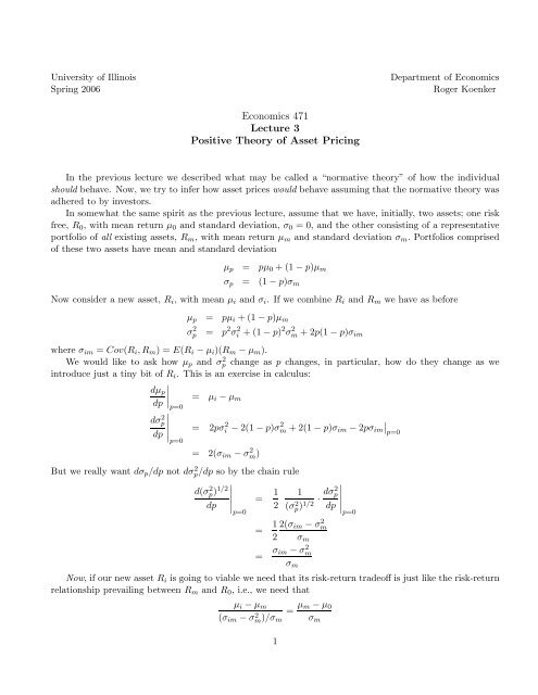
University of IllinoisSpring 2006Department of EconomicsRoger KoenkerEconomics 471Lecture 3Positive Theory of Asset PricingIn the previous lecture we described what may be called a “normative theory” of how the individualshould behave. Now, we try to infer how asset prices would behave assuming that the normative theory wasadhered to by investors.In somewhat the same spirit as the previous lecture, assume that we have, initially, two assets; one riskfree, R 0 , with mean return µ 0 and standard deviation, σ 0 = 0, and the other consisting of a representativeportfolio of all existing assets, R m , with mean return µ m and standard deviation σ m . Portfolios comprisedof these two assets have mean and standard deviationµ p = pµ 0 + (1 − p)µ mσ p= (1 − p)σ mNow consider a new asset, R i , with mean µ i and σ i . If we combine R i and R m we have as beforeµ p = pµ i + (1 − p)µ mσ 2 p= p 2 σ 2 i + (1 − p) 2 σ 2 m + 2p(1 − p)σ imwhere σ im = Cov(R i ,R m ) = E(R i − µ i )(R m − µ m ).We would like to ask how µ p and σp 2 change as p changes, in particular, how do they change as weintroduce just a tiny bit of R i . This is an exercise in calculus:dµ pdpdσ 2 pdp∣ = µ i − µ mp=0= 2pσi 2 − 2(1 − p)σ 2 ∣m + 2(1 − p)σ∣ im − 2pσ ∣p=0 imp=0= 2(σ im − σ 2 m )But we really want dσ p /dp not dσp 2 /dp so by the chain ruled(σp 2)1/2= 1 1dp ∣ 2 (σ 2 · dσ2 p∣p=0p )1/2 dp= 1 2(σ im − σm22 σ m= σ im − σ 2 mσ mNow, if our new asset R i is going to viable we need that its risk-return tradeoff is just like the risk-returnrelationship prevailing between R m and R 0 , i.e., we need thatµ i − µ m(σ im − σ 2 m)/σ m= µ m − µ 0σ m1∣p=0

orSubtract µ m − µ 0 to both sides to obtain,(σim − σ 2 )mµ i − µ m = (µ m − µ 0 )µ i − µ 0 = (µ m − µ 0 )σ 2 m(σimThis is a fundamental relationship – what does it say? Very simply it says that expected excess returns ofasset i,µ i − µ 0 , is proportional to the expected excess returns on the market portfolio, µ m − µ 0 , with factorof proportionality σ im /σm 2 . The latter factor is a regression coefficient.Suppose we have the classical bivariate linear regression modely i = α + βx i + u iand we estimate α and β by minimizing the sum of squared deviations of the y i ’s from the estimated line,that is we solve∑min (yi − α − βx i ) 2α,βThe solution isˆβ =ˆα = ȳ − ˆβ¯xσ 2 m∑ (yi − ȳ)(x i − ¯x)∑ (xi − ¯x) 2we can interpret ˆβ as an estimate that simply a ratio of estimates of the covariance of x and y to the estimateof the variance of x.Looking back at our fundamental CAPM relationship we see that this precisely what our factor σ im /σ 2 mis – the ratio of covariance of R i and R m to the variance of R m . This yields the basic model,)(∗)R it − R 0t = α + β(R mt − R 0t ) + u twhere β now represents σ im /σm 2 . Of course in the model we derived α = 0, so we need to consider this abit further. But the basic message is simple: Expected returns of R i given market returns follows a simple,linear regression model.The regression formulation of our CAPM relationship yields a variety of new insights. The expectedexcess return, µ i − µ 0 , is sometimes called the risk premium of asset R i since it measures how much abovethe risk free rate of return the expected return on R i needs to be to justify its uncertain return. Similarly,µ m − µ 0 is the risk premium for the market portfolio. The coefficient β can then be viewed as establishinga connection between the risk premium of asset, R i , and the risk premium of the market as a whole. If β isgreater (less) than one, then R i has a larger (smaller) risk premium than the market risk premium.The regression formulation (∗) allows us to decompose the variance of R i into a portion attributed tovariation in the market and a portion independent of the market,σ 2 R = β2 σ 2 M + σ2 u .So if we take variance as a measure of risk we can view the first component as risk associated with the marketthat can’t be avoided, and the second component as risk that can be avoided by diversification. To seehow the latter works imagine a large number, n, of stocks that have random contributions u 1t ,u 2t ,... ,u nt2

independent of the market return. For simplicity suppose that we form a portfolio with equal portfolioweights, 1/n, thenV (ū t ) = V ( 1 n∑u it ) = 1 ∑σ2n n 2 iAs long as the σ 2 i are all roughly the same magnitude, say σ 2 i ≤ σ2 0i=1V (ū t ) ≤ σ 2 0/nfor all i, thenso for large n the contribution of these components to the portfolio variance is small.On the other hand, the portion of the variance associated with the market can’t be diversified away.Assets with β > 1 have variability that magnifies the market variation and they – according to the CAPMtheory – can expect to earn a large risk premium to compensate. Assets with β < 1 vary less violently thanthe market as a whole and therefore earn less than the market rate of return.What if β ≤ 0? If β = 0, the model predicts that ER i = µ 0 , that is that the asset should earn the riskfree rate of return; this is true because in this case there is only diversifiable risk. When β < 0 the situationis even more extreme: when the market goes up the expectation is that such assets go down and vice-versa.This makes them ideal diversification investments: when the market declines they tend to soften the blow.Unfortunately such assets are hard to find. In some periods gold has shown some tendency to exhibit anegative β. This is explored in the last part of the first problem set.Finally, a word about α in the regression model (∗). As derived, α should take the value zero. If whenwe estimate the model we see an ˆα > 0 it means that over the estimation period the asset in question hadreturns that exceeded that predicted by the CAPM, and likewise if ˆα < 0 its performance was worse thanpredicted. Of course, when estimating such models from historical data, ˆα’s are always non zero, what ismore important is to ask: how strong is the evidence that α ≠ 0. Typically this evidence is very weak.3