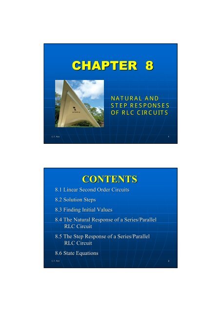
8.4 The Natural Response of a Series/Parallel RLC Circuit

8.1 Linear Second Order Circuits• Circuits containing two energy storage elements.• Described by differential equations that containsecond order derivatives.• Need two initial conditions to get the uniquesolution.C.T. Pan 38.1 Linear Second Order Circuits• Examples(a) RLC parallel circuit(b) RLC series circuitis() t+vt ()−vs() tit ()C.T. Pan 4

8.1 Linear Second Order Circuits(c) 2L+R , RL circuitR1R2vs() tL L12(d) 2C+R , RC circuitRis() tC 1C 2C.T. Pan 58.2 Solution StepsStep1 : Choose nodal analysis or meshanalysis approachStep2 : Differentiate the equation as manytimes as required to get the standardform of a second order differentialequation .2d x dxa + b + x=yt ()2dt dtC.T. Pan 6

8.3 Finding Initial ValuesUnder transient condition, L is like an open circuitand C is like a short circuit because i L (t) ) and v C (t)are continuous functions if the input is bounded.C.T. Pan 98.3 Finding Initial ValuesUnder transient condition, L is like an open circuitand C is like a short circuit because i L (t) ) and v C (t)are continuous functions if the input is bounded.C.T. Pan 10

8.3 Finding Initial Values• Example 1 (cont.)t < 0∴ i(0 + ) = i(0 - ) = 2 Av(0 + ) = v(0 - ) = 4 Vi(0 - ) = 2 Av(0 - ) = 4 VC.T. Pan 138.3 Finding Initial Values• Example 1 (cont.)t = 0 ++di d + VL(0 )Q L = VL, ∴ i(0 ) =dt dt L+dv d + iC(0 )QC= iC, ∴ v(0 ) =dt dt CC.T. Pan 14

8.3 Finding Initial Values• Example 1 (cont.)+KVL: 2A× 4 + v (0 ) + 4V = 12V+∴ v (0 ) = 0d i+∴ (0 ) = 0dt+KCL: i (0 ) = 2ACLLd v+∴ (0 ) = 0dt+iC(0 ) 2∴ = = 20 V/SC 0.1C.T. Pan 158.3 Finding Initial Values• Example 1 (cont.)4Ω 0.25Hi2Ω12V0.1F + v-t=0t →∞L is short circuitdC is open∴i( ∞ ) = 0v( ∞ ) = 12VC.T. Pan 16

• Example 28.3 Finding Initial Values4Ω3u(t)A 2Ω__ 12 F ++ vcv R --0.6H20Vi L+ d +Find : ( a) iL(0 ) , iL(0 ) , iL( ∞)dt+ d +( b) vC(0 ) , vC(0 ) , vC( ∞)dt+ d +() c vR(0 ) , vR(0 ) , vR( ∞)dtC.T. Pan 178.3 Finding Initial Values• Example 2 (cont.)4Ω3u(t)A 2Ω1__2 F ++ vcv R --0.6H20Vi Lt < 02Ω+v R-4Ω20V+v c-i L−∴ i (0 ) = 0L−v (0 ) =−20VvcR−(0 ) = 0C.T. Pan 18

8.3 Finding Initial Values• Example 2 (cont.)4Ω3u(t)A 2Ω__ 12 F ++ vcv R --0.6H20Vi L t = 0 ++ −∴ i (0 ) = i (0 ) = 0LL+ −v (0 ) = v (0 ) =−20VccC.T. Pan 198.3 Finding Initial Values• Example 2 (cont.)4Ω3u(t)A 2Ω__ 12 F ++ vcv R --0.6H20V3A2Ωt = 0 ++ v o (0 + ) -4Ω+v R (0 + )-i c (0 + )i L+ 4i2Ω(0 ) = 3A× = 2A2+4+vR(0 ) = 2A× 2=4V+ 2ic(0 ) = 3A× = 1A2+4+d vL(0 ) 0i+∴L(0 ) = = = 0dt L L+d + ic(0 ) 1vc(0 ) = = = 2dt c 1 2d v+R(0 ) = ?dtC.T. Pan 20VS

8.3 Finding Initial Values• Example 2 (cont.)4Ω3u(t)A 2Ω__ 12 F ++ vcv R --0.6H20Vi L t > 0 +3A2Ω+ v o -4Ω1__ + i L+ 2 F vcv R-- 0.6H20VFrom KVL: − v + v + v + 20=0R o cTake derivatived d dvR() t = vo() t + vc()tdt dt dtd + d + d +∴ vR(0 ) = vo(0 ) + vc(0 ) LL( A)dt dt dtC.T. Pan 218.3 Finding Initial Values• Example 2 (cont.)4Ω3u(t)A 2Ω__ 12 F ++ vcv R --0.6H20Vi L t > 0 +3A2Ω+ v o -4Ω1__ + i L+ 2 F vcv R-- 0.6H20VvR()t vo()tAlso , from KCL: 3A= +2 4Take derivative1 d 1 d0 = vR() t + vo() t LL(B)2 dt 4 dtC.T. Pan 22

8.3 Finding Initial Values• Example 2 (cont.)d + d +From ( B) vo(0 ) =−2 vR(0 ) LL( C)dt dtFrom ( A) and ( C)d + d +vR(0 ) =− 2 vR(0 ) + 2dtdtd 2 v+∴ (0 ) VR=dt 3 SC.T. Pan 238.3 Finding Initial Values• Example 2 (cont.)4Ω3u(t)A 2Ω__ 12 F ++ vcv R --0.6H20Vi Lt →∞3A2Ω4Ω+v R ( )-+v c ( )-20Vi L2∴iL( ∞ ) = 3A× = 1A2+4v ( ∞ ) =−20Vcv ( ∞ ) = 3 A× (2ΩP4 Ω ) = 4VRC.T. Pan 24

8.4 The Natural Response of a Series/ParallelRLC Circuit(a) The source-free series RLC circuitThis section is an important background for studyingfilter design and communication networks .initial conditions⎧i(0)= I0⎨⎩v(0)= V0C.T. Pan 258.4 The Natural Response of a Series/ParallelRLC Circuitinitial conditions⎧i(0)= I0⎨⎩v(0)= V0Step 1 : Mesh analysisdi 1 tRi+ L + idt 0dt C∫=−∞To eliminate the integral , take derivative2di di 12dt dt CL + R + i = 0C.T. Pan 26

8.4 The Natural Response of a Series/ParallelRLC Circuitinitial conditions⎧i(0)= I0⎨⎩v(0)= V0Step 2 : Homogeneous solution , characteristic equation2 R 1S + S+ =0L LC2 2 R 2 1S +2αS+ω0=0 ⇒ α @ , ω0@2L LCω : undamped resonant frequency (rad/s)0α : damping factor or neper frequencyC.T. Pan 278.4 The Natural Response of a Series/ParallelRLC Circuitinitial conditions⎧i(0)= I0⎨⎩v(0)= V0characteristic roots (natural frequencies)S =-α+ α -ω2 21 0S =-α- α -ω2 22 0St 1 St 2() 1 2∴ i t = Ae + Ae+ d +Need two initial conditions , i.e. , i(0 ) and i(0 ) .diC.T. Pan 28

8.4 The Natural Response of a Series/ParallelRLC CircuitCase 1 Overdamped Case ( α > ω )Two real rootsSt 1 St 2() =1+2i t Ae AeCase 2 Critically Damping Case ( α= ω )Equal real rootsRS1 = S2=− =−α2Li t = A + At e −αt() ( )2 100C.T. Pan 298.4 The Natural Response of a Series/ParallelRLC CircuitCase 3 Underdamped Case ( α < ω )Complex conjugate rootsSS12=− α + jω()dd=−α− jωω @ ω −αd2 20−αti t = e B cosωt+B sinω1 d 20damping frequency( )Once i(t) is obtained ,solutions of other variables can beobtained from this mesh current.dtC.T. Pan 30

8.4 The Natural Response of a Series/ParallelRLC Circuit• The damping effect is due to the presence of resistance R .• The damping factor α determines the rate at which theresponse is damped .• If R=0 , the circuit is said to be lossless and theoscillatory response will continue .• The damped oscillation exhibited by the underdampedresponse is known as ringing . It stems from the ability ofthe L and C to transfer energy back and forth betweenthem .C.T. Pan 318.4 The Natural Response of a Series/ParallelRLC CircuitStep 3 : Initial Condition+ + −t = 0, i(0 ) = i(0 ) = IFrom mesh equation , let t = 0+1 0+ d +Ri(0 ) + L i(0 ) + idt 0dt C∫=−∞d + R + V0R∴ i(0 ) =− i(0 ) − =− Idt L L L0+0V0−LC.T. Pan 32

8.4 The Natural Response of a Series/ParallelRLC Circuitor from equivalent circuit at t=0d +L i(0 ) = vL=− ( IR0+ V0)dtd IR0Vi+0∴ (0 ) =− −dt L L+RI 0v LV 0iC.T. Pan 338.4 The Natural Response of a Series/ParallelRLC Circuit(b) The source-free parallel RLC circuitinitial inductor current I oinitial capacitor voltage V oStep 1 : Nodal Equationv 1 t dv+ vdt C 0R L∫+ =dtTaking derivative to eliminate the integral2dv 1 dv 1+ + v = 02dt RC dt LCC.T. Pan 34

8.4 The Natural Response of a Series/ParallelRLC CircuitStep 2 : Homogeneous solutionCharacteristic equation2 1 1S + S+ = 0RC LC2 2 1 2 1S + 2αS+ ω0 = 0 ⇒ α @ , ω0@2RCLCcharacteristic roots ( naturalfrequencies)SS=− α + α −ω2 21 0=−α − α −ω2 22 0C.T. Pan 358.4 The Natural Response of a Series/ParallelRLC CircuitCASE 1. Overdamped Case (α>w(>w 0 )St 1 2( ) = +v t Ae Ae1 2CASE 2. Critically Damped Case (α=w(0 )( ) = ( + )1 2CASE 3. Underdamped Case (α

8.4 The Natural Response of a Series/ParallelRLC CircuitStep 3 : Initial Condition+ −v(0 ) = i(0 ) = VFrom nodal equation+( )+( )C.T. Pan 370v 0+1 0 d ++ vdt C v( 0 ) 0R L∫+ =−∞dtv 0+d1 0+∴ C v( 0 ) =− − vdtdt R L∫−∞V0=− −I0Rd V0 Iv+0∴ ( 0 ) =− −dt RC C8.4 The Natural Response of a Series/ParallelRLC Circuitor from equivalent circuit at t=0d + +C v(0 ) = iC( 0 )dt+d iC(0 )v+∴ (0 ) =dt C+ V0From KCL, iC(0 ) =−I0−ROnce the nodal voltage is obtained, any other unknownof the circuit can be found .+C.T. Pan 38

8.5 The Step Response of a Series/Parallel RLCCircuit(a) Step response of a seriesRLC circuitStep 1. Mesh analysis (i=i L )di 1L + Ri+ idt = Vs, t > 0dt C∫Case(i) take derivatived 2i + Rdi + i = 02Ldt dt CC.T. PanSame as natural response but with i(0 + )=I 0+ Vs−IR 0−V0( 0 ) =39d idtL8.5 The Step Response of a Series/Parallel RLCCircuitCase(ii) use v as unknowndvi = C dt2dv Rdv v V+ + = s2dt Ldt LC LCStep 2. Complete solution = v h +v pph( )v t = VsSt 1 St 2⎧ Ae1+ Ae2overdamped⎪v t A At e critically damped−αt() = ⎨( 1+2 )⎪ −αt( cos + sin )⎩e A1 wtdA2wtdunderdampedC.T. Pan 40

8.5 The Step Response of a Series/Parallel RLCCircuitStep 3. Initial conditions+ −( 0 ) ( 0 )v = v = Vd vdtdvC+( )0 = ?= idtC0+( 0 ) I0d iCv+∴ ( 0 ) = =dt C CThen the unique solution can be determinedC.T. Pan 418.5 The Step Response of a Series/Parallel RLCCircuit(b) Step response of a parallel RLC circuitI 0 , V 0 GivenStep 1.Nodal equationv 1 t dv+ vdt C Is, t 0R L∫+ = >dtCase (i) Take derivativeC2dv 1 dv 12dt Rdt L+ + v=0Same as natural responseC.T. Pan 42

8.5 The Step Response of a Series/Parallel RLCCircuitCase (ii) Let2di di 1 di 1 I s2dt dt RC dt LC LCv= L ⇒ + + i = , t > 0Step 2. Complete solution = i h (t)+i p (t)Step 3.ph( )i t = IsSt 1 St 2⎧ Ae1+ Ae2overdamped⎪i t A At e critically damped−αt() = ⎨( 1+2 )⎪ −αt( cos + sin )⎩e A1 wtdA2wtdundererdampedInitial Condition+ −( 0 ) ( 0 )i = i = I0di d vL ( 0)(0)+Vdt dt L L+0C.T. Pan L = vL⇒ i = =438.5 The Step Response of a Series/Parallel RLCCircuit• Example1 F2- -t < 0 , i(0 )=0 , v(0 ) =12Vt>01 F2C.T. Pan44

8.5 The Step Response of a Series/Parallel RLCCircuitC.T. PanMethod (a)v 1 dvFrom KCL ⇒ i = +2 2 dt(A)diFrom KVL ⇒ 4i+ 1 + v = 12dt(B)Substitute (A) into (B)2dv 1 dv 1 d v(2v+ 2 )+( + )+ v= 122dt 2 dt 2 dt2⇒ d v dv5 6v24V2dt+ dt+ =Characteristic equation( s+ 2)( s+ 3) = 0s=− 2, s =−31 2458.5 The Step Response of a Series/Parallel RLCCircuitv () t = A e + A eh−2t−3t1 224vp() t = = 4V6∴ vt () = 4+ A e + A e−2t−3t1 2+ -Initial Condition v(0 )= v(0 )=12V+t=01 F2C.T. PandvC = icdt++dv(0 ) ic(0 ) −646∴ = = =−12 V/Sdt C 1/2

8.5 The Step Response of a Series/Parallel RLCCircuit∴ 4+ A + A = 121 2−2A − 3A =−121 2∴ A = 12, A =−41 2∴ vt = + e − e t ≥2 3() 4 12 − t − t4 , 0Method (b) Using Mesh Analysist>04Ωi1HC.T. Pan12V2Ω1i 1 i 2v F2478.5 The Step Response of a Series/Parallel RLCCircuitdi1 + 4 i+ ( i1− i2)2=12 ......(A)dt1 t( i2 − i1) × 2Ω+ 20 ......(B)1/2∫idt =di2 di1From (B) , 2 − 2 + 2i2= 0dt dtdi+ 6i1− 2i2= 12dtdi1 di2− 2 + 2 + 2i2= 0dt dt1 F2C.T. Pan48

8.5 The Step Response of a Series/Parallel RLCCircuitdIn matrix form with operator D@dt⎡D+ 6 −2 ⎤⎡i1⎤ ⎡12⎤⎢ =− 2D2D+2⎥⎢ i⎥ ⎢20⎥⎣ ⎦⎣ ⎦ ⎣ ⎦(C)C.T. Pan+ + −Initial Condition , i (0 ) = i(0 ) = i(0 ) = 0A+ +i (0 ) = i (0 ) =−6A2c+ +di1(0 ) vL(0 )= = 0dt L+di2(0 )= 0 A/Sdt1498.5 The Step Response of a Series/Parallel RLCCircuitEliminate ivariable from (C)2di1 di1+ 5 + 6i21= 12dt dt∴ i t = − e + e t ≥−2t−3t1() 2 6 4 , 0Or eliminate i2variable from (C)2di2 di2+ 5 + 6i22= 0dt dt∴ i t =− e + e t ≥1−2t−3t2() 12 6 , 0C.T. Pan50

8.5 The Step Response of a Series/Parallel RLCCircuitProblem : (a) Time consuming to eliminate the othervariable to get a higher order differentialequation.(b) It is also necessary to obtain the desiredinitial conditions.(c) As the order gets higher when thenetwork contains more energy storageelements, the process gets morecomplicated.The difficulty can be overcome by using state equationformulation.C.T. Pan518.6 State EquationWhen the differential equations of a circuit is written inthe following form:d x = f ( xut , ,)dtTx = [ x x .... x ] state vectorT1 2u = [ u u .... u ] input vector1 2Tf = [ f f .. f ] vector function1 2nnmC.T. Pan52

8.6 State EquationIt is said that the circuit equations are in the stateequation form.(a) This form lends itself most easily to analog or digitalcomputer programming.(b) The extension to nonlinear and/or time varyingnetworks is quite easy.(c) In this form, a number of theoretic concepts ofsystems are readily applicable to networks.C.T. Pan 53For a linear time-invarying circuit , a simpler formd x = A x + B u , state equationdty= Cx+D u , output equationA : n×n matrix.B : n×m matrix.C :8.6 State Equationl×n matrix.D: l × m matrix.Note that on the right hand side of the state or outputequation, only x and u are allowed.C.T. Pan54

8.6 State EquationStep1. Pick a tree which contains all the capacitors andnone of inductors.Step2. Use the tree-branch capacitor voltages and thelink inductor currents as unknown (i.e. , state)variables.Note: (a) Nodal AnalysisEvery unknown of the circuit can becalculated from nodal voltages.(b) Mesh AnalysisEvery unknown of the circuit can becalculated from mesh currents.C.T. Pan558.6 State Equation(c) State Equation• The chosen variables include bothvoltage and current unknown. It belongsto mixed type.• Every unknown of the circuit can becalculated from the state variables byreplacing each inductor with a currentsource and each capacitor with a voltagesource and then solving the resultingresistive circuit.C.T. Pan56

8.6 State EquationStep3. Write a fundamental cutset equation (i.e. KCLequation) for each capacitor.Note that in these cutsetequations, all branchcurrents must be expressed in terms of x and u.Step4. Write a fundamental loop equation (i.e. KVLequation) for each inductor.Note that in these loop equations, all branchvoltages must be expressed in terms of x and u.Step5. Rearrange the above equations into standard formand find the solution for the given initial condition.C.T. Pan57•Example 18.6 State EquationStep1treeC.T. Pan58

8.6 State EquationStep2 choose i and v as state variables.Step3 fundamental cutsetabout the capacitor tree branch.dvvC = i -dt 2Step4 fundamental loop for the inductor link.C.T. PandiL + v -12V +4 i = 0dt598.6 State EquationStep5⎡ 1 -1 ⎤⎡0⎤d ⎡v⎤ ⎢C 2C⎥⎡v⎤ = + ⎢1⎥ (12V)dt⎢i⎥ ⎢ ⎥-4 -1⎢i⎥⎣ ⎦ ⎢ ⎥⎣ ⎦ ⎢ ⎥⎢⎣L⎦⎣LL ⎥⎦[ A ] [ B]The desired solutions are v and i⎡v⎤ ⎡1 0⎤⎡v⎤ ⎡0⎤y = ⎢ = + (12V)i⎥ ⎢0 1⎥⎢i⎥ ⎢0⎥⎣ ⎦ ⎣ ⎦⎣ ⎦ ⎣ ⎦[ C ] [ D]with initial condition +v(0 ) = 12V+i(0 ) = 0AC.T. Pan 60

•Example 2C.T. Pan8.6 State Equation3 2d v d v dv+5 +4 +3 v=u(t)3 2dt dt dt⎧⎧ dx1⎪=xx21= v(t)⎪dt⎪⎪⎪ d(t) v ⎪ dx2Let ⎨x 2= ⇒ ⎨ =x3⎪ dt ⎪ dt2 3⎪ d v(t) ⎪dx3d v⎪x 3= =3 ⎪3⎩ dt ⎩ dt dt2d v dv= -5 - 4 -3 v+u(t)2dt dt61= -5x - 4x -3x +u(t)3 2 1State space representation8.6 State Equation⎡x1⎤ ⎡0 1 0⎤⎡x1⎤⎡0⎤d ⎢ x⎥ =⎢ 0 0 1⎥⎢ x⎥ +⎢ 0⎥ u(t)⎢ ⎥ ⎢ ⎥x ⎢⎣-3 -4 -5⎥⎦ x ⎢⎣1⎥⎦⎡x1⎤y = [ 1 0 0⎢] x⎥2+0u(t)⎢ ⎥[ ]⎢⎣x3⎥⎦∴2 2dt ⎢ ⎥ ⎢ ⎥⎢⎣ 3⎥⎦ ⎢⎣ 3⎥⎦A high order differential equation can be representedin the form of state equation.C.T. Pan62

• Example 3 : Find v R48.6 State Equationai 3Ri 43C 1L 1 L 2b hi L1 i L2g R 1e scR 2 R 4+- v C1d+C 2- v C2efR 5There are 8 nodes.C.T. Pan 638.6 State EquationStep1 Pick a tree as follows :ai L1i L2gbhC.T. Panc+ dv C1- +e -fv C2There are 7 tree branchesand 3 links.64

8.6 State EquationStep2 Choose i L1 , i L2 , v C1 , v C2 as unknowns.Step3 Fundamental cutsets (KCL) for capacitors.dvC1C1= iL1dtdvC2C2= iL1+iL2dtStep4 Fundamental loops (KVL) for inductors.diL1L1= -vR1- vC1- vC2- vR5 + vR4dt= -R i - v - v - R ( i + i ) + v1L1 C1 C2 5 L1 L2 R4Note that v R4 should be expressed in terms of x and uC.T. Pan658.6 State EquationAbsorb voltages v R1and v C1 in currentsource i L1 ,and v R2 in i L2 .Absorb voltages v C2and v R5 in (i L1 + i L2 )current source.C.T. Pan66

8.6 State EquationR∴v = e - ( i + i )RR43 4R4 s L1 L2R+R3 4R+R3 4C.T. Pan67Step5⎡1⎤⎢0 0 0C ⎥10⎢⎥⎡ ⎤⎡vC1⎤ ⎢1 1 ⎥ ⎡vC1⎤⎢0⎥⎢ 0 0d v⎥ ⎢C2 C2 C⎥ ⎢2 v⎥⎢ ⎥⎢ ⎥ C2 1 R= ⎢⎥ ⎢ ⎥⎢ ⎥+ 4 esdt ⎢iL1⎥ ⎢⎢1 1 (R1 R 2)R iL1L⎥− − − + − ⎥ ⎢ ⎥ 1 R 3+R4⎢ ⎥ ⎢⎥ ⎢ ⎥⎢ ⎥⎣iL2⎦ ⎢L1 L1 L1 L1⎥ ⎣iL2⎦ ⎢ 1 ⎥⎢⎢ ⎥−1 −R− (R2+ R) ⎥ L0⎣ 2 ⎦⎢⎥⎣ L2 L2 L2⎦C.T. Pan8.6 State Equation⎡vC1⎤⎡ -R3R4 -R3R4 ⎤⎢v⎥C2 Rv4R4 = ⎢0 0 ⎥ ⎢ ⎥ + es⎣ R3 + R4 R3 + R4⎦ ⎢ iL1⎥ R3 + R4⎢ ⎥⎣iL2⎦RRwhere R @ R 3 45 + R 3 +R 468

Special case8.6 State Equation(a)i 1 i 3i 2From KCLi 1 +i 2 +i 3 = 0∴ i 3 = -i 1 -i 2Inductor current i 3 is dependent on i 1 and i 2 andis no longer a state variable.One can choose only n-1 (here 2) inductorcurrents as state variables.C.T. Pan698.6 State Equation(b)From KVLv C1 +v C2 = v C3One can choose n-1 (here 2) capacitorvoltages as state variables.C.T. Pan70

Summary• Objective 1 : Be able to find the initial values and theinitial derivative values.• Objective 2 : Be able to determine the natural responseand the step response of a series RLC circuit.• Objective 3 : Be able to determine the natural responseand the step response of a parallel RLC circuit.• Objective 4 : Be able to obtain the state equation andoutput equation of a linear circuit.C.T. Pan 71SummaryChapter Problems : 8.168.258.328.408.44Due within one week.C.T. Pan 72