A Short Introduction to Classical and Quantum Integrable Systems

A SHORT INTRODUCTION TO CLASSICAL AND QUANTUM INTEGRABLE SYTEMS.O. BabelonLaboratoire de Physique Théorique et Hautes Energies 1 , (LPTHE)Unité Mixte de Recherche UMR 7589Université Pierre et Marie Curie-Paris6; CNRS; Université Denis Diderot-Paris7;20071 Tour 24-25, 5ème étage, Boite 126, 4 Place Jussieu, 75252 Paris Cedex 05.

DIRECTION DES SCIENCES DE LA MATIÈRESERVICE DE PHYSIQUE THÉORIQUEUnité de recherche associée au CNRSCOURS DE PHYSIQUE THÉORIQUE DU SPHTANNÉE 2006-2007Les vendredis de 14h30 à 16h30 au SPhT, Orme des Merisiers, Bat.774, Salle ItzyksonPetite introduction aux systèmesintégrables classiques et quantiquesDu 19 janvier au 16 février 2007Organisé en commun avec l’École Doctorale de Physique de la Région Parisienne (ED107)Olivier BABELONLab. de Phys. Théoriqueet Hautes EnergiesUniversités Paris VI et VIILe but de ce cours est d'introduire les méthodes analytiques de résolution des systèmesintégrables classiques et quantiques.Systèmes classiques:1- Paires de Lax, orbites coadjointes, matrice r classique.2- Courbe spectrale, linéarisation du flot sur la jacobienne, variables séparées.3- Théorie des champs, matrice de monodromie, solitons, solutions finite zones.Systèmes quantiques:4- Modèle de Gaudin, Ansatz de Bethe.5- Des équations de Bethe a la courbe spectrale. Limite semi classique.6- Chaine XXX, Ansatz de Bethe, équation de Baxter. Chaine de Toda...Les cours sont de nature introductive et accessibles aux étudiants en deuxième année de troisièmecycle. Ils sont ouverts aux physiciens de toute discipline et à toute personne intéressée.Pour tout renseignement : www-spht.cea.fr ou lectures@spht.saclay.cea.fr

Contents1 Integrable dynamical systems 71.1 The Liouville theorem . . . . . . . . . . . . . . . . . . . . . . . . . . . . . 71.2 Lax pairs . . . . . . . . . . . . . . . . . . . . . . . . . . . . . . . . . . . . 101.3 The Zakharov-Shabat construction. . . . . . . . . . . . . . . . . . . . . . . 101.4 Coadjoint Orbits. . . . . . . . . . . . . . . . . . . . . . . . . . . . . . . . . 141.5 Classical r-matrix. . . . . . . . . . . . . . . . . . . . . . . . . . . . . . . . 181.6 Examples. . . . . . . . . . . . . . . . . . . . . . . . . . . . . . . . . . . . . 211.6.1 The Jaynes-Cummings-Gaudin model. . . . . . . . . . . . . . . . . 211.6.2 The KdV hierarchy. . . . . . . . . . . . . . . . . . . . . . . . . . . 252 Solution by analytical methods 312.1 The spectral curve. . . . . . . . . . . . . . . . . . . . . . . . . . . . . . . . 312.2 Riemann surfaces. . . . . . . . . . . . . . . . . . . . . . . . . . . . . . . . 322.2.1 Desingularisation . . . . . . . . . . . . . . . . . . . . . . . . . . . . 322.2.2 Riemann-Hurwitz theorem. . . . . . . . . . . . . . . . . . . . . . . 342.2.3 Riemann-Roch theorem. . . . . . . . . . . . . . . . . . . . . . . . . 352.2.4 Jacobi variety and Theta functions. . . . . . . . . . . . . . . . . . 362.3 Genus of the spectral curve. . . . . . . . . . . . . . . . . . . . . . . . . . . 402.4 Dimension of the reduced phase space. . . . . . . . . . . . . . . . . . . . . 412.5 The eigenvector bundle. . . . . . . . . . . . . . . . . . . . . . . . . . . . . 432.6 Separated variables. . . . . . . . . . . . . . . . . . . . . . . . . . . . . . . 462.7 Riemann surfaces and integrability. . . . . . . . . . . . . . . . . . . . . . . 492.8 Solution of the Jaynes-Cummings-Gaudin model. . . . . . . . . . . . . . . 522.8.1 Degenerate case. . . . . . . . . . . . . . . . . . . . . . . . . . . . . 532.8.2 Non degenerate case . . . . . . . . . . . . . . . . . . . . . . . . . . 563 Infinite dimensional systems. 673.1 Integrable field theories and monodromy matrix. . . . . . . . . . . . . . . 673.2 Abelianization. . . . . . . . . . . . . . . . . . . . . . . . . . . . . . . . . . 693.3 Poisson brackets of the monodromy matrix. . . . . . . . . . . . . . . . . . 723.4 Dressing transformations. . . . . . . . . . . . . . . . . . . . . . . . . . . . 743.5 Soliton solutions. . . . . . . . . . . . . . . . . . . . . . . . . . . . . . . . . 763.5.1 KdV solitons. . . . . . . . . . . . . . . . . . . . . . . . . . . . . . . 785

3.6 Finite zones solutions. . . . . . . . . . . . . . . . . . . . . . . . . . . . . . 803.7 The Its-Matveev formula. . . . . . . . . . . . . . . . . . . . . . . . . . . . 814 The Jaynes-Cummings-Gaudin model. 894.1 Physical context. . . . . . . . . . . . . . . . . . . . . . . . . . . . . . . . . 894.1.1 Rabi oscillations. . . . . . . . . . . . . . . . . . . . . . . . . . . . . 894.1.2 Cold atoms condensates. . . . . . . . . . . . . . . . . . . . . . . . . 924.2 Settings. . . . . . . . . . . . . . . . . . . . . . . . . . . . . . . . . . . . . . 934.3 Bethe Ansatz. . . . . . . . . . . . . . . . . . . . . . . . . . . . . . . . . . . 954.4 Riccati equation. . . . . . . . . . . . . . . . . . . . . . . . . . . . . . . . . 994.5 Baxter Equation. . . . . . . . . . . . . . . . . . . . . . . . . . . . . . . . . 1024.6 Bethe eigenvectors and separated variables. . . . . . . . . . . . . . . . . . 1044.7 Quasi-Classical limit. . . . . . . . . . . . . . . . . . . . . . . . . . . . . . . 1084.8 Riemann surfaces and quantum integrability. . . . . . . . . . . . . . . . . 1105 The Heisenberg spin chain. 1175.1 The quantum monodromy matrix . . . . . . . . . . . . . . . . . . . . . . . 1175.2 The XXX spin chain. . . . . . . . . . . . . . . . . . . . . . . . . . . . . . . 1185.3 Algebraic Bethe Ansatz. . . . . . . . . . . . . . . . . . . . . . . . . . . . . 1235.3.1 Baxter equation. . . . . . . . . . . . . . . . . . . . . . . . . . . . . 1275.3.2 Separated variables. . . . . . . . . . . . . . . . . . . . . . . . . . . 1296 Nested Bethe Ansatz. 1356.1 The R-matrix of the Affine sl n+1 algebra. . . . . . . . . . . . . . . . . . . 1356.2 sl n+1 generalization of the XXZ model. . . . . . . . . . . . . . . . . . . . 1366.3 Commutation relations. . . . . . . . . . . . . . . . . . . . . . . . . . . . . 1376.4 Reference state. . . . . . . . . . . . . . . . . . . . . . . . . . . . . . . . . . 1386.5 Bethe equations. . . . . . . . . . . . . . . . . . . . . . . . . . . . . . . . . 1416

Chapter 1Integrable dynamical systemsThe usually accepted definition of an integrable system in the sense of Liouville is asystem with phase space of dimension 2n for which one knows n conserved quantities ininvolution. This a rather puzzling definition since by Darboux theorem one can alwaysfind locally a system of canonical coordinates on phase space (P 1 , · · · , P n ; Q 1 , · · · , Q n )with H = P 1 hence fulfilling the hypothesis of Liouville theorem. However the genericdynamical system is certainely not what we mean by integrable system, so the hypothesismust be made more precise by requiring some global existence properties of the conservedquantities. A good starting point is to ask, following Moser, that the conserved quantitiesexist on an open domain of the phase space invariant under the dynamical flow, that isany trajectory starting in the domain stays in it.In all the examples that we will consider the conserved quantities are even analyticfunctions of canonical coordinates on some open domain and the known solutions aresimilarly analytic.1.1 The Liouville theoremWe consider a dynamical hamiltonian system with phase space M, dim M = 2n. Introducecanonical coordinates p i , q i such that the non degenerate Poisson bracket reads{p i , q j } = δ ij . As usual a non degenerate Poisson bracket on M is equivalent to the dataof a non-degenerate closed 2-form ω, dω = 0, defined on M. In the canonical coordinatesω = ∑ j dp j ∧ dq j . Let H be the hamiltonian of the system. For any function f on M,the equations of motion are Hamilton’s equations:dfdt ≡ f ˙ = {H, f}Here and in the following, a dot will refer to a time derivative.Definition 1 The system is Liouville integrable if it possesses n independent conservedquantities F i , i = 1, · · · , n, {H, F j } = 0, in involution,{F i , F j } = 07

There cannot be more than n independent quantities in involution otherwise the Poissonbracket would be degenerate. In particular, the hamiltonian H is a function of the F i ’s.Theorem 1 (The Liouville theorem.) The solution of the equations of motion of anintegrable system is obtained by quadrature.Proof. Let α = ∑ i p idq i be the canonical 1-form and ω = dα = ∑ i dp i ∧ dq i be thesymplectic 2-form on the phase space M. We will construct a canonical transformation(p i , q i ) → (F i , Ψ i ) such that the F i ’s are among the new coordinates. i.e., a transformationsuch thatω = ∑ dp i ∧ dq i = ∑ dF i ∧ dΨ iiiIf we succeed to do that, the equations of motion become trivial:Their solutions are:˙ F j = {H, F j } = 0˙ψ j = {H, ψ j } = ∂H∂F j= Ω j (F ).F j (t) = F j (0)ψ j (t) = ψ j (0) + tΩ j .To construct this canonical transformation, we exhibit its generating function S. LetM f be the level manifold F i (p, q) = f i . Suppose we can solve for p i , p i = p i (f, q), andconsider the functionS(F, q) =∫ mm 0α =∫ qq 0∑ip i (f, q)dq i ,where the integration path is drawn on M f and goes from the point of coordinate(p(f, q 0 ), q 0 ) to the point (p(f, q), q), where q 0 is some reference value.If this function exists, i.e. if it does not depend on the path from m 0 to m, it is thefunction we are looking for. Indeed, from the definition of S, p j = ∂S∂q j. Defining ψ j byψ j = ∂S∂F j,we havedS = ∑ jψ j dF j + p j dq j ,Since d 2 S = 0 we deduce that ω = ∑ j dp j ∧ dq j = ∑ j dF j ∧ dψ j . This shows that if Sis a well defined function then the transformation is canonical.8

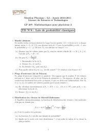
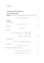
Figure 1.1: Integration path on the level manifold M f .To show that S exists, we must prove that it is independent of the integration path, ie.we have to prove thatdα| Mf = ω| Mf = 0Let X i be the hamiltonian vector field associated to F i , defined by dF i = ω(X i , ·),X i = ∑ k∂F i∂q k∂∂p k− ∂F i∂p k∂∂q k.These vector fields are tangent to the manifold M f because the F j are in involution,X i (F j ) = {F i , F j } = 0Since the F j are assumed to be independent functions, the tangent space to the submanifoldM f is generated at each point m ∈ M by the vectors X i | m (i = 1, . . . , n). But thenω(X i , X j ) = dF i (X j ) = 0 and we have proved that ω| Mf = 0, and therefore S exists.Remark. From the closedness of α on M f , the function S is unchanged by continuousdeformations of the path (m 0 , m). However, if M f has non trivial cycles, which isgenerically the case, S is a multivalued function defined in a neighborhood of M f . Thevariation over a cycle∫∆ cycle S = αis a function of F only. This induces a multivaluedness of the variables ψ j : ∆ cycle ψ j =∂∂F j∆ cycle S.9cycle

1.2 Lax pairsThe new concept which emerged from the modern studies of integrable systems is thenotion of Lax pairs. A Lax pair L, M consists of two functions on the phase space of thesystem, with values in some Lie algebra G, such that the hamiltonian evolution equationsmay be written asdLdt ≡ ˙L = [M, L](1.1)Here, [ , ] denotes the bracket in the Lie algebra G. We will denote by G the connectedLie group having G as a Lie algebra.Although eq.(1.1) only requires a Lie algebra structure to be written down, we usuallyuse finite dimensional representations of G, so that L and M are matrices. However itwill be important to keep in mind the more abstract formulation.The interest in the existence of such a pair originates in the fact that it allows for aneasy construction of conserved quantities. Indeed the solution of eq(1.1) is of the formL(t) = g(t)L(0)g −1 (t)where g(t) ∈ G is determined by the equationM = dgdt g−1It follows that the eigenvalues of L are conserved. We say that the evolution equation(1.1) is isopsectral which means that the spectrum of L is preserved by the time evolution.Alternatively the quantitiesare conserved.H n = Tr (L n )Integrability of the system in the sense of Liouville demands (i) that the system isHamiltonian, (ii) that the number of independent conserved quantities equals the numberof degree of freedom, and (iii) that these conserved quantities are in involution.The interest in the concept of Lax pairs relies on the existence of a tool allowing toproduce such pairs fulfilling these constraints.1.3 The Zakharov-Shabat construction.Given an integrable system, there does not yet exists a useful algorithm to construct aLax pair. There does exist however a general procedure, due to Zakharov and Shabat, toconstruct consistent Lax pairs giving rise to integrable systems. This is a general method10

to construct matrices L(λ) and M(λ), depending on a spectral parameter λ ∈ C, suchthat the Lax equation∂ t L(λ) = [M(λ), L(λ)] (1.2)is equivalent to the equations of motion of an integrable system. The main result iseq.(1.13) expressing the possible forms of the matrix M in the Lax pair.Let us consider matrices L(λ) and M(λ) of dimension N × N. We will assume thatthe matrices L(λ) and M(λ) are rational functions of the parameter λ. Let {ɛ k } bethe set of their poles, namely the poles of L(λ) and those of M(λ). With the abovenotations, assuming no pole at infinity, we can write quite generally:andL(λ) = L 0 + ∑ kM(λ) = M 0 + ∑ kL k (λ), with L k (λ) ≡M k (λ) with M k (λ) ≡∑−1r=−n kL k,r (λ − ɛ k ) r (1.3)∑−1r=−m kM k,r (λ − ɛ k ) r (1.4)Here n k and m k refer to the order of the poles at the corresponding point ɛ k . Thecoefficients L k,r and M k,r are matrices. We will assume that the positions of the polesɛ k are constants independent of time.We now want to impose that the Lax equation (1.2), with L(λ) and M(λ) given byeqs.(1.3,1.4), holds identically in λ. It is important to realize that this is a very nontrivial equation. Indeed looking at eqs.(1.2) we see that the pole at ɛ k in the left handside is a priori of order n k while in the right hand side it is potentially of order n k + m k .Hence we have two types of equations. The first type does not contain time derivativesand comes from setting to zero the coefficients of the poles of order greater than n k inthe right hand side of the equation. This will be interpreted as m k constraint equationson M k . The equations of the second type are obtained by matching the coefficients ofthe poles of order less or equal to n k on both sides of the equation. These equationscontain time derivatives and are thus the true dynamical equations. It turns out thatone can solve the constraints equations.We introduce a notation. For any matrix valued rational function f(λ) with poles oforder n k at points ɛ k at finite distance, we can decompose f(λ) asf(λ) = f 0 + ∑ kf k (λ), with f k (λ) =∑−1r=−n kf k,r (λ − ɛ k ) r ,with f 0 a constant. The quantity f k (λ) is called the polar part at ɛ k . When there is noambiguity about the pole we are considering, we will often use the alternative notationf − (λ) ≡ f k (λ). Around one of the point ɛ k , f(λ) may be decomposed as follows:f(λ) = f(λ) + + f(λ) − (1.5)11

with f(λ) + regular at the point ɛ k and f(λ) − = f k (λ) is the polar part.Assuming that L(λ) has distinct eigenvalues in a neighbourhood of ɛ k , one can performa regular similarity transformation g (k) (λ) diagonalizing L(λ) in a vicinity of ɛ k .L(λ) = g (k) (λ) A (k) (λ) g (k)−1 (λ) (1.6)where A (k) (λ) is diagonal and has a pole of order n k at ɛ k . Obviously, we can write thepolar decomposition of L(λ) asL = L 0 + ∑ kL k , with L k =(g (k) A (k) g (k)−1) −(1.7)A first consequence of the Lax equation is that M(λ) admits a similar polar decompositionProposition 1 The decomposition of M(λ) in polar parts readsM = M 0 + ∑ kM k , with M k =(g (k) B (k) g (k)−1) −(1.8)where B (k) (λ) is diagonal and has a pole of order m k at ɛ k .Proof.Defining B (k) (λ) bythe Lax equation becomes:M(λ) = g (k) (λ) B (k) (λ) g (k)−1 (λ) + ∂ t g (k) (λ) g (k)−1 (λ) (1.9)˙ A (k) (λ) = [B (k) (λ), A (k) (λ)]This implies A ˙ (k) = 0 as expected (because the commutator with a diagonal matrix hasno element on the diagonal), and moreover if we assume that the diagonal elements ofA (k) are all distinct this equation implies that B (k) is also diagonal. Finally the term∂ t g (k) g (k)−1 is regular and does not contribute to the singular part M k of M at ɛ k . HenceM k = (g (k) B (k) g (k)−1 ) − which only depends on B (k)− . This simultaneous diagonalizationof L(λ) and M(λ) works around any point where L(λ) has distinct eigenvalues.This proposition clarifies the structure of the Lax pair. Only the singular parts ofA (k) and B (k) contribute to L k and M k . The independent parameters in L(λ) are thusL 0 , the singular diagonal matrices A (k)−A (k)−1− = ∑of the formr=−n kA k,r (λ − ɛ k ) r (1.10)12

and jets of regular matrices ĝ (k) of order n k − 1, defined up to right multiplication by aregular diagonal matrix d (k) (λ):ĝ (k) =n∑k −1r=0g k,r (λ − ɛ k ) r (1.11)From these data, we can reconstruct the Lax matrix L(λ) by defining L = L 0 + ∑ k L kwith(L k ≡ ĝ (k) A (k)−(1.12)ĝ(k)−1)−Then around each ɛ k , one can diagonalize L(λ) = g (k) A (k) g (k)−1 . This yields an extensionof the matrices A (k)− and ĝ(k) to complete series A (k) and g (k) in (λ − ɛ k ). Finally todefine M(λ) = M 0 + ∑ k M k, we choose a set of diagonal polar matrices (B (k) (λ)) − anduse the series g (k) to define M k by eq.(1.8).In the vicinity of a singularity, L(λ) and M(λ) can be simultaneously diagonalizedif the Lax equation holds true. In this diagonal gauge, the Lax equation simply statesthat the matrix A (k) (λ) is conserved and that B (k) (λ) is diagonal. When we transformthese results into the original gauge, we get the general solution of the non dynamicalconstraints on M(λ):Proposition 2 Let L(λ) be a Lax matrix of the form eq.(1.3). The general form of thematrix M(λ) such that the orders of the poles match on both sides of the Lax equationis M = M 0 + ∑ k M k withM k =( )P (k) (L, λ)−where P (k) (L, λ) is a polynomial in L(λ) with coefficients rational in λ and (the singular part at λ = ɛ k .(1.13)) −denotesProof. It is easy to show that this is indeed a solution. We have to check that the orderof the poles is correct. Let us look at what happens around λ = ɛ k . Using a beautifulargument first introduced by Gelfand and Dickey we write:[M k , L] − ==[ (P (k) (L, λ))− , L ][(]P (k) (L, λ) − P (k) (L, λ))+ , L−−[ ( ]= − P (k) (L, λ))+ , L −where we used that a polynomial in L commutes with L. From this we see that the orderof the pole at ɛ k is less than n k . To show that this is a general solution, recall eqs. (1.6,13

1.8). Since A (k) (λ) is a diagonal N × N matrix with all its elements distinct in a vicinityof ɛ k , its powers 0 up to N − 1 span the space of diagonal matrices and one can writeB (k) = P (k) (A (k) , λ) (1.14)where P (k) (A (k) , λ) is a polynomial of degree N − 1 in A (k) . The coefficients of P (k)are rational combinations of the matrix elements of A (k) and B (k) hence admit Laurentexpansions ( in λ −)ɛ k in a vicinity of ɛ k . Inserting eq. (1.14) into eq. (1.8) one getsM k = P (k) (L, λ) . Moreover in this formula the Laurent expansions of the coefficients−of P (k) can be truncated at some positive power of λ − ɛ k since a high enough powercannot contribute to the singular part, yielding a polynomial with coefficients Laurentpolynomials in λ − ɛ k .The above propositions give the general form of M(λ) as far as the matrix structureand the λ–dependence is concerned. One should keep in mind however that the coefficientsof the polynomials P (k) (L, λ) are a priori functions of the matrix elements of Land require further characterizations in order to get an integrable system. In the settingof the next section these coefficients will be constants.Remark. The Lax equation is invariant under similarity transformations,L → L ′ = gLg −1 , M → M ′ = gMg −1 + ∂ t gg −1 (1.15)If this similarity transformation is independent of λ, it will not spoil the analytic propertiesof L(λ) and M(λ). We can use the gauge freedom eq.(1.15) to diagonalize L 0 ,L 0 = Diag(a 1 , · · · , a N )Consistency of eq.(1.2) then requires M 0 to be also diagonal and thus ˙L 0 = [M 0 , L 0 ] = 0.Hence M 0 is a polynomial P of L 0 , so that replacing M(λ) → M(λ) − P (L(λ)) gets ridof M 0 .1.4 Coadjoint Orbits.In this section we show that the Zakharov–Shabat construction, when the matrices A (k)−are non dynamical, can be interpreted as coadjoint orbits. This introduces a naturalsymplectic structure in the problem and gives a Hamiltonian interpretation to the Laxequation.Let G be a connected Lie group with Lie algebra G. The group G acts on G by theadjoint action denoted Ad:X −→ (Ad g)(X) = gXg −1g ∈ G, X ∈ GSimilarly the coadjoint action of G on the dual G ∗ of the Lie algebra G (i.e. the vectorspace of linear forms on the Lie algebra) is defined by:(Ad ∗ g.Ξ)(X) = Ξ(Ad g −1 (X)),g ∈ G, Ξ ∈ G ∗ , X ∈ G14

The infinitesimal version of these actions provides actions of the Lie algebra G on G andG ∗ denoted ad and ad ∗ respectively and given by:ad X(Y ) = [X, Y ] X, Y ∈ G,ad ∗ X.Ξ(Y ) = −Ξ([X, Y ]) X, Y ∈ G, Ξ ∈ G ∗On the space F(G ∗ ) of functions on G ∗ there is a canonical Poisson bracket calledthe Kostant-Kirillov bracket. Let Ξ ∈ G ∗ and X, Y ∈ G, we define{Ξ(X), Ξ(Y )} = Ξ([X, Y ])(1.16)If e a is a basis of G and e ∗a is the dual basis of G ∗ , then we haveX = ∑ aX a e a ∈ G,Ξ a e ∗a ∈ G ∗Ξ = ∑ aandSetting X = e a , Y = e b in eq.(1.16) we findΞ(X) = ∑ Ξ a X a{Ξ a , Ξ b } = f abc Ξ cwhere we have introduced the structure constants of the Lie algebra G[e a , e b ] = f abc e cThis formula define the Poisson bracket of the coordinates Ξ a on G ∗ . We can extend iton the functions on G ∗ (i.e. functions of the Ξ a ) in the usual way{F, G}(Ξ) = ∑ a,bIntroducing the differentials dF, dG ∈ G asdF dG{Ξ a , Ξ b } = ∑ dF dGΞ c f abcdΞ a dΞ b dΞ a dΞ ba,b,cdF (Ξ) = ∑ adFdΞ ae a ,dG(Ξ) = ∑ bdGdΞ be bthe above formula can be rewritten in the more invariant way{F, G}(Ξ) = Ξ([dF, dG])The Kostant-Kirillov bracket is degenerate, meaning that there exists functions whichPoisson commutes with everything. For instance if the basis e a is chosen so that thestructure constants f abc are totally antisymmetric the functionΞ 2 = ∑ aΞ 2 a15

is in the center of the Poisson bracket. Indeed{Ξ 2 , Ξ b } = 2 ∑ a,cf abc Ξ a Ξ c = 0In the context of Hamiltonian mechanics, it is important to identify all such functionsand to set them to constants since they cannot contribute to the dynamics. This iswhere the notion of coadjoint orbit plays a very important role. The coadjoint orbit ofan element A ∈ G ∗ is the set of elements of G ∗ defined asOrbit(A) = {Ad ∗ g · A, ∀g ∈ G}The center of the Kostant-Kirillov bracket consists of the functions which are Ad ∗ -invariant, i.e. which are constant on coadjoint orbits. In fact for such a function wehaveF (Ξ) = F (Ad ∗ g · Ξ)Taking an infinitesimal g = 1 + ɛX, this translates toF (Ξ) = F (Ξ + ɛ ad ∗ X · Ξ) = F (Ξ) + ɛ ad ∗ X · Ξ(dF ) + O(ɛ 2 )hence, the Ad ∗ -invariance of F (Ξ) can be written asad ∗ X · Ξ(dF ) = Ξ([dF, X]) = 0,∀X ∈ GOn the other hand, if F (Ξ) is in the kernel of the Kostant-Kirillov bracket we have{F (Ξ), Ξ(X)} = Ξ([dF, X]) = 0, ∀X ∈ Gso that the Ad ∗ -invariant functions are in the kernel and vice versa. On coadjoint orbits,the Kostant-Kirillov bracket becomes non degenerate.To see how these notions relate to our problem, let us consider first a Lax matrixwith only one polar singularity at λ = 0:L(λ) =()g(λ) A − (λ) g −1 (λ)−with A − (λ) = ∑ −1r=−n A rλ r , and g(λ) has a regular expansion around λ = 0.(1.17)Let G be the loop group of invertible matrix valued power series expansion aroundλ = 0. The elements of G are regular series g(λ) = ∑ ∞r=0 g r λ r . The product law isthe pointwise product: (gh)(λ) = g(λ)h(λ). Formally, the Lie algebra G of G consistsof elements of the form X = ∑ ∞r=0 X r λ r . Its Lie bracket is given by the pointwisecommutator.16

The dual G ∗ of G can be identified with the set of polar matrices Ξ(λ) = ∑ r≥1 Ξ r λ −r ,where the sum contains a finite but arbitrary large number of terms, by the pairing:〈Ξ, X〉 ≡ Tr Res λ=0 (Ξ(λ)X(λ)) = ∑ rTr (Ξ r+1 X r )where Res λ=0 is defined to be the coefficient of λ −1 .The coadjoint action of G on G ∗ is defined by ((Ad ∗ g) · Ξ) (X) = Ξ(g −1 Xg) forΞ ∈ G ∗ and any X ∈ G. Using the above model for G ∗ , and since 〈Ξ, g −1 Xg〉 =〈gΞg −1 , X〉 = 〈(gΞg −1 ) − , X〉, we get(Ad ∗ g) · Ξ(λ) = ( g · Ξ · g −1) −This is precisely eq.(1.17). The Lax matrix can thus be interpreted as belonging to thecoadjoint orbit of the element A − (λ) of G ∗ under the loop group G.()L(λ) = g(λ) A − (λ) g −1 (λ) = Orbit(A −(λ))−If we take any element of the orbit and try to diagonalize it, the singular part of thematrix of eigenvalues is precisely A − (λ) which is therefore an Ad ∗ -invariant function andshould be put to constants. This interpretation of L(λ) as a coadjoint orbit thereforeassumes that A − (λ) is not a dynamical variable. The coadjoint orbit is then equippedwith the Kostant-Kirillov symplectic structure.This construction can be extended to the multi–pole case. We consider the directsum of loop algebras G k , around λ = ɛ k :G ≡ ⊕ kG kAn element of this Lie algebra has the form of a multipletX(λ) = (X 1 (λ), X 2 (λ), · · ·)where X k (λ), defined around ɛ k , is of the form X k (λ) = ∑ n≥0 X k,n (λ − ɛ k ) n . The Liebracket is such that [X k (λ), X l (λ)] = 0 if k ≠ l. The group G is the direct product ofthe groups G k of regular invertible matrices at ɛ k :The dual G ∗ of this Lie algebra consists of multipletsG ≡ (G 1 , G 2 , · · ·) (1.18)Ξ = (Ξ 1 (λ), Ξ 2 (λ), · · ·)17

where Ξ k (λ) around ɛ k is of the form Ξ k (λ) = ∑ r≥1 Ξ k,r(λ − ɛ k ) −r . In this sum thenumber of terms is finite but arbitrary. The pairing is simply〈Ξ, X〉 ≡ ∑ k〈Ξ k , X k 〉 = ∑ kTr Res ɛk (Ξ k (λ)X k (λ))The coadjoint action of G on G ∗ is given by the usual formula: if g = (g 1 , g 2 , · · ·) ∈ Gand Ξ = (Ξ 1 , Ξ 2 , · · ·) ∈ G ∗(Ad ∗ g).Ξ(λ) = ((g 1 Ξ 1 g −11 ) −, (g 2 Ξ 2 g −12 ) −, · · ·)A coadjoint orbit consists of elements Ξ k with a fixed maximal order of the pole. Then,we can interpret eq.(1.7) as the coadjoint orbit of the element ((A 1 ) − , (A 2 ) − , · · ·).Alternatively, we can consider the function on G ∗L(λ) = L 0 + ∑ kΞ k (1.19)with poles at the points ɛ k . Given this function we can recover the Ξ k by extracting thepolar parts. The constant matrix L 0 is added to match the formula for the Lax matrixeq.(1.7). By choice it is assumed to be invariant by coadjoint action. The pairing canbe rewritten as〈L, X〉 = ∑ Tr Res ɛk L(λ)X k (λ)kRemark that only Ξ k contributes to the residue at ɛ k and the formula is compatible withthe matrix L 0 being invariant by coadjoint action.1.5 Classical r-matrix.We can now use this symplectic form to evaluate the Poisson brackets of the elements ofthe Lax matrix and show that they take the r–matrix form. Let us first introduce somenotations. Let E ij be the canonical basis of the N × N matrices, (E ij ) kl = δ ik δ jl . Wecan writeL(λ) = ∑ L ij (λ)E ijijLetL 1 (λ) ≡ L(λ) ⊗ 1 = ∑ ijL ij (λ)(E ij ⊗ 1),L 2 (µ) ≡ 1 ⊗ L(µ) = ∑ ijL ij (µ)(1 ⊗ E ij )The index 1 or 2 means that the matrix L sits in the first or second factor in the tensorproduct. More generally when we have tensor products with more copies, we denote byL α the embedding of L in the α position, e.g. L 3 = 1 ⊗ 1 ⊗ L ⊗ 1 ⊗ · · ·. Finally, we define{L 1 (λ), L 2 (µ)} as the matrix of Poisson brackets between the elements of L:{L 1 (λ), L 2 (µ)} = ∑ ij,kl{L ij (λ), L kl (µ)}E ij ⊗ E kl18

We assume that each L k (λ) is a generic element of an orbit of the loop groupGL(N)[λ] that L 0 and the A (k)− are non–dynamical. Each orbit L k(λ) is equipped withthe Kostant-Kirillov Poisson bracket and{L k (X), L k ′(Y )} = 0, k ≠ k ′ (1.20)Proposition 3 With these assumptions, the Poisson brackets of the matrix elements ofL(λ) can be written as:[ ]C12{L 1 (λ), L 2 (µ)} = −λ − µ , L 1(λ) + L 2 (µ)(1.21)with C 12 = ∑ i,j E ij⊗E ji where the E ij are the canonical basis matrices. The commutatorin the right hand side of eq.(1.21) is the usual matrix commutator.Proof. Let us first assume that we have only one pole and L = (gA − g −1 ) − . Becausewe are dealing with a Kostant-Kirillov bracket for the loop algebra of gl(N), we canimmediately write the Poisson bracket of the Lax matrix using the defining relation{L(X), L(Y )} = L([X, Y ]). Using, L(X) = Tr Res λ=0 (L(λ)X(λ)), this gives:{L(X), L(Y )} = Tr Res λ=0 (L(λ)[X(λ), Y (λ)]) (1.22)By definition of the notation {L 1 , L 2 }, we have:{L(X), L(Y )} = 〈{L 1 (λ), L 2 (µ)} , X(λ) ⊗ Y (µ)〉where 〈, 〉 = Tr 12 Res λ Res µ . We need to factorize X(λ) ⊗ Y (µ) in eq.(1.22). To this end,we introduce the operator, assuming |λ| < |µ|,:C 12 (λ, µ) = C 12∞ ∑n=0λ nµ n+1 = − C 12λ − µ ,C 12 = ∑ i,jE ij ⊗ E jiThis operator is such that for Y (λ) = ∑ ∞n=0 Y nλ n we haveWe can now write:Y 1 (λ) = Tr 2 Res µ C 12 (λ, µ)Y 2 (µ)〈L(λ)[X(λ), Y (λ)]〉 = 〈[C 12 (λ, µ), L(λ) ⊗ 1] , X(λ) ⊗ Y (µ)〉Consider the rational function of λ: ϕ(λ) = {L 1 (λ), L 2 (µ)} − [C 12 (λ, µ), L(λ) ⊗ 1]. Byinspection ϕ contains only negative powers of µ, and we have 〈ϕ, X(λ) ⊗ Y (µ)〉 = 0.Hence ϕ contains only positive powers of λ and is regular at λ = 0. It has a pole atλ = µ, due to the form of C(λ, µ). We remove this pole by subtracting to ϕ the quantity[C 12 (λ, µ), 1⊗L(µ)] which contains only positive powers of λ and is therefore in the kernel19

of 〈·, X(λ) ⊗ Y (µ)〉. The pole at λ = µ disappears since [C 12 , L(µ) ⊗ 1 + 1 ⊗ L(µ)] = 0.The redefined ϕ is regular everywhere and vanishes for λ → ∞ hence vanishes identically.This proves eq.(1.21) in the one-pole case.We can now study the multi–pole situation occuring in eq.(1.7). Consider L =L 0 + ∑ k L k. Each L k lives in a coadjoint orbit as above equipped with its own symplecticstructure. From eq.(1.20) they have vanishing mutual Poisson brackets{(L k (λ)) 1 , (L k ′(µ)) 2 } = 0, k ≠ k ′We assume further that L 0 does not contain dynamical variables{(L 0 ) 1 , (L 0 ) 2 } = 0, {(L 0 ) 1 , (L k (λ)) 2 } = 0Then since C 12 /(λ − µ) is independent of the pole ɛ k , it is obvious that the r-matrix relationsfor each orbit combine by addition to give eq.(1.21) for the complete Lax matrixL(λ).We have obtained a very simple formula for the r-matrix specifying the Poissonbracket of L(λ):r 12 (λ, µ) = −r 21 (µ, λ) = − C 12(λ − µ)(1.23)The Jacobi identity is satisfied because this r-matrix verifies the classical Yang–Baxterequation[r 12 , r 13 ] + [r 12 , r 23 ] + [r 13 , r 23 ] = 0where r ij stands for r ij (λ i , λ j ). Note that r 12 is antisymmetric: r 12 (λ 1 , λ 2 ) = −r 21 (λ 2 , λ 1 ).These Poisson brackets for the Lax matrix ensure that one can define commutingquantities. The associated equations of motion take the Lax form.Proposition 4 The functions on phase space:H (n) (λ) ≡ Tr( )L n (λ)are in involution. The equations of motion associated to H (n) (µ) can be written in theLax form with M = ∑ k M k:M k (λ) = −n( L n−1 )(λ)λ − µk(1.24)20

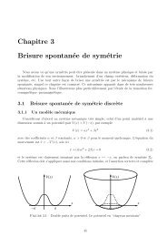
Proof.The quantities H (n) (λ) are in involution because{Tr L n (λ), Tr L m (µ)} = nmTr 12 {L 1 (λ), L 2 (µ)}L n−11 (λ)L m−12 (µ)= − nmλ − µ Tr 12 ([C 12 , L n 1 (λ)]L m−12 (µ) + [C 12 , L m 2 (µ)]L1 n−1 (λ)) = 0where we have used that the trace of a commutator vanishes. Similarly, we have:[ ]˙L(λ) = {H (n) C12(µ), L(λ)} = nTr 2λ − µ Ln−1 2 (µ), L 1 (λ)Performing the trace and remembering that Tr 2 (C 12 M 2 ) = M 1 , we get˙L(λ) = [M (n) (λ, µ), L(λ)], M (n) (λ, µ) = n Ln−1 (µ)λ − µ(1.25)This M (n) (λ, µ) has a pole at λ = µ and is otherwise regular. According to the generalprocedure we can remove this pole by subtracting some polynomial in L(λ) withoutchanging the equations of motion. Obviously one can redefine:M (n) (λ, µ) → M (n) (λ, µ) − n Ln−1 (λ)λ − µ = (λ) − L n−1 (µ)−nLn−1λ − µ(1.26)This new M has poles at all ɛ k and is regular at λ = µ. Decomposing it into its polarparts, we write M = ∑ k M k with( L n−1 )(λ)M k (λ) = −nλ − µkThis is of the form eq.(1.13) withP (k) (L, λ) = −nλ − µ Ln−1 (λ) (1.27)Notice that the coefficients of the polynomial P (k) (L, λ) are pure numerical constants.This proposition shows that the generic Zakharov-Shabat system, equipped withthis symplectic structure, is an integrable Hamiltonian system (the precise counting ofindependent conserved quantities will be done in Chapter [2]).1.6 Examples.1.6.1 The Jaynes-Cummings-Gaudin model.We consider the following Hamiltoniann−1∑n−1∑H = 2ɛ j s z −j + ω¯bb + g(¯bsjj=0j=021+ bs + j)(1.28)

The ⃗s j are spins variables, and b, ¯b is a harmonic oscillator. The Poisson brackets read{s a j , s b j} = −ɛ abc s c j, {b, ¯b} = i (1.29)The ⃗s j brackets are degenerate. We fix the value of the Casimir functions⃗s j · ⃗s j = s 2Phase space has dimension 2(n + 1). The equations of motion readWe introduce the Lax matricesn−1∑ḃ = −iωb − ig s − j(1.30)j=0ṡ z j = ig(¯bs − j − bs+ j ) (1.31)ṡ + j= 2iɛ j s + j − 2ig¯bs z j (1.32)ṡ − j= −2iɛ j s − j + 2igbsz j (1.33)L(λ) = 2 g 2 λσz + 2 g (bσ+ + ¯bσ − ) − ω n−1∑ ⃗s j · ⃗σg 2 σz +(1.34)λ − ɛ jM(λ) = −iλσ z − ig(bσ + + ¯bσ − ) (1.35)where σ a are the Pauli matrices.j=0σ ± = 1 2 (σx ± iσ y ), [σ z , σ ± ] = ±2σ ± , [σ + , σ − ] = σ zIt is not difficult to check that the equations of motion are equivalent to the Lax equation˙L(λ) = [M(λ), L(λ)] (1.36)Letwe have( )A(λ) B(λ)L(λ) =C(λ) −A(λ)A(λ) = 2λg 2 − ω n−1g 2 + ∑B(λ) = 2b n−1g + ∑j=0C(λ) = 2¯b n−1g + ∑22j=0j=0s − jλ − ɛ js + jλ − ɛ js z jλ − ɛ j

It is very simple to check that{A(λ), A(µ)} = 0{B(λ), B(µ)} = 0{C(λ), C(µ)} = 0{A(λ), B(µ)} =i(B(λ) − B(µ))λ − µ{A(λ), C(µ)} = − i (C(λ) − C(µ))λ − µ{B(λ), C(µ)} =2i(A(λ) − A(µ))λ − µOne can rewrite these equations in the usual form[ ]P12{L 1 (λ), L 2 (µ)} = −iλ − µ , L 1(λ) + L 2 (µ)where⎛⎞1 0 0 0P 12 = ⎜ 0 0 1 0⎟⎝ 0 1 0 0 ⎠0 0 0 1It follows that12 Tr (L2 (λ)) = A 2 (λ) + B(λ)C(λ)generates Poisson commuting quantities. One has12 Tr L2 (λ) = 1 g 4 (2λ − ω)2 + 4 g 2 H n + 2 n−1∑g 2where the (n + 1) Hamiltonians readj=0n−1H j∑+λ − ɛ jj=0⃗s j · ⃗s j(λ − ɛ j ) 2 (1.37)H n = b¯b + ∑ js z jandH j = (2ɛ j − ω)s z j + g(bs + j+ ¯bs − j ) + g2 ∑ k≠js j · s kɛ j − ɛ k, j = 0, · · · , n − 1The Hamiltonian eq.(1.28) isn−1∑H = ωH n +Let us see how these formulae fit into our general scheme. The Lax matrix is a sumof simple poles at ɛ j . The loop group at each one of these points isj=0H jg (j) (λ) = g (j)0 + (λ − ɛ j )g (j)1 + · · ·23

where g (j)kthe coadjoint orbit.are SU(2) matrices. In fact the pole being simple, only g (j)0 contributes toL j (λ) =(g (j) (λ)At infinity we consider the loop groupsσ z )g (j)−1 (λ) = s g (j)0λ − ɛ j −λ − ɛ σz g (j)−10jg (∞) (λ) = 1 + λ −1 g (∞)−1 + · · ·and the coadjoint orbitL ∞ (λ) = 2 )(g (∞)g 2 (λ) λσ z g (∞)−1 (λ) = 2 + g 2 λσz + 2 g 2 [g(∞) −1 , σz ] ≡ 2 g 2 λσz + 2 g (bσ+ +¯bσ − )IdentifyingL 0 = − ω g 2 σzwe do haven−1∑L(λ) = L 0 + L ∞ (λ) + L j (λ)To see how M(λ) also fits into the scheme, we consider separately the evolution withrespect to the Hamiltonians H j , H n . Since H j is the coefficient of2g 2 (µ−ɛ j ) in 1 2 Tr L2 (µ)we just have to extract this coefficient in eq.(1.26), which for n = 2 reads (there is anextra factor i coming from the definition of the Poisson bracket)We findj=0M (2) L(λ) − L(µ)(λ, µ) = −iλ − µM j (λ) = i g22⃗s j · ⃗σλ − ɛ jSimilarly, for ωH n we have to extract the term in µ 0 in the same expression. We findHenceM(λ) = M ∞ (λ) + M j (λ) = i g22M ∞ (λ) = −i ω 2 σz (1.38)⎛⎝− ω g 2 σz +n−1∑j=0⎞⃗s j · ⃗σ⎠λ − ɛ j(= −i λσ z + g(bσ + + ¯bσ) − ) + i g22 L(λ)Since the L(λ) term does not contribute to the Lax equation, we have recovered theexpression eq.(1.35) for the matrix M(λ).24

1.6.2 The KdV hierarchy.In the one pole case, we have seen that the general structure of a Lax equation is[ ( ]˙L(λ) = P (L, λ))− , L(λ) (1.39)The KdV hierarchies are constructed exactly on the same pattern but replacing loopalgebras by the algebra of pseudo differential operators which we now describe.The algebra of pseudo-differential operators is the algebra of elements of the formA =N∑i=−∞with N finite but arbitrary. The coefficients a i are functions of x, ∂ is the usual derivationwith respect to x and the “integration” symbol, ∂ −1 is defined by the following algebraicrules:We denote by P =Let P + ={A = ∑ −1a i ∂ i∂ −1 ∂ = ∂∂ −1 = 1∞∑∂ −1 a = (−1) i (∂ i a)∂ −i−1 (1.40)i=0{A = ∑ N−∞ a i∂ i }the set of formal pseudo-differential operators.{A = ∑ Ni=0 a i∂ i }be the subalgebra of differential operators, and let P − =}−∞ a i∂ i be the subalgebra of integral operators.decomposition of P as a vector space:We have the direct sumP = P + ⊕ P −Notice that P is naturally a Lie algebra. P + and P − are Lie subalgebras. but P + andP − do not commute.The formal group G = exp(P − ) is called the Volterra group. We have G ∼ 1 + P −because powers of elements in P − are in P − . Let Φ be an element of G:Φ = 1 +∞∑w i ∂ −i ∈ (1 + P − ) (1.41)i=1The coefficients of its inverse Φ −1 = 1 + ∑ ∞1 w′ i ∂−i can be computed recursively fromthe relation Φ −1 Φ = 1.25

For A ∈ P we define its residue, denoted Res ∂ A, as the coefficient of ∂ −1 in A:Res ∂ A ≡ a −1 (x)(1.42)On P there exists a natural linear form called the Adler trace, denoted 〈 〉, defined by:∫〈A〉 =∫dx Res ∂ A =dx a −1 (x)(1.43)This linear form satisfies the fundamental trace property 〈AB〉 = 〈BA〉.Returning to integrable systems, we now let L be a differential operator of order nn−2∑L = ∂ n − u i ∂ i (1.44)In the algebra of pseudo differential operators its n-th root existsi=0Q = L 1 n , Q = ∂ + q−1 ∂ −1 + · · ·The generalized KdV hierarchies are defined by the Lax equations (compare witheq.(1.39). In both cases the projection is on the dual of the Lie algebras G[λ] and P −respectively.)[ ( ]∂ tk L = L k n)+ , L(1.45)These equations are consistent for all k ∈ IN in the sense that we have a differentialoperator of order n − 2 on both side. To see it, we notice that Q k , ∀k ∈ N commuteswith L since LQ k = Q n+k = Q k L. Then, we have:[ (Q k) + , L ]=[ ]Q k , L −[ (Q k) − , L ][ (= − Q k) ], L−[ (QFrom the last equality, it follows that the differential operatork ) ]+ , L is of order lessor equal to n − 2, so that the Lax equation eq.(1.45) is an equation on the coefficientsof L. This is the original Gelfand-Dickey argument.The differential operator L is an element of P + . If we view P + as the dual of theLie algebra P − through the Adler trace, there is a natural Poisson bracket on P + : theKostant–Kirillov bracket. For any functions f and g on P + , it is defined as usual by:{f, g}(L) = 〈L , [df, dg]〉 ∀ L ∈ P + (1.46)26

where we understand that df, dg ∈ P − . In particular, for any X = ∑ ∞j=0 ∂−j−1 x j ∈ P − ,we define the linear function f X (L) by:f X (L) = 〈L, X〉 (1.47)we have df X = X ∈ P − . Therefore {f X , f Y } = 〈L, [X, Y ]〉 = f [X,Y ] for any X, Y ∈ P − .Proposition 5 Let L ∈ P + be the differential operator of order n as in eq.(1.44). Definethe functions of L byH k (L) = 11 + k n〈L k n +1 〉(i) The functions H k (L) are the Hamiltonians of the generalized KdV flows under thebracket eq.(1.46):[ ( ]∂ tk L = {H k , L} = L k n)+ , L (1.48)(ii) The functions H k (L) are in involution with respect to this bracket.Proof. We first need to compute the differential of the Hamiltonian H k . Let L and δLbe differential operators of the form eq.(1.44). One has, using the cyclicity of Adler’strace:〈(L + δL) ν 〉 = 〈L ν 〉 + ν〈L ν−1 δL〉 + · · ·which implies d〈L ν 〉 = ν(L ν−1 ) (−n) where the notation ( ) (−n) means projection on P −truncated at the first n − 1 terms. This projection appears because δL = −δu n−2 ∂ n−2 −· · · − δu 0 which is dual to elements of the form ∂ −1 x 0 + · · · + ∂ −n+1 x n−1 under the Adlertrace. Hence:((dH k (L) = L k n)(−n) = Q k) ∈ P − (1.49)(−n)We call θ (k)−(n)the terms left over in the truncation:( )L k n = dH k + θ (k)−−(n)(1.50)We now prove eq.(1.48). Consider the function f X (L) = 〈LX〉, then˙ f X = 〈 ˙L, X〉 = {H k , f X }(L) = 〈L, [dH k , df X ]〉 = 〈[L, dH k ], X〉where we used the invariance of the Adler trace. Since X ∈ P − , only [L, dH k ] + contributesto this expression. But[ ( ) ] [ ] [ ( ][L, dH k ] + = L, L k n − L, θ (k)−−(n)= L k n+)+ , L+where we have used [L k n , L] = 0, and the fact that [L, θ (k)−(n) ] + = 0. So [L, dH k ] + is adifferential operator of order at most n − 2, and this proves eq.(1.48).27

Next we show that the Hamiltonians H k are in involution. We have:{H k , H k ′}(L) = 〈L, [dH k , dH k ′]〉 = 〈[L, dH k ] + , dH k ′〉( ]= 〈[L k n)+ , L , dH k ′〉Using again the fact that [L, dH k ] + is of order at most n − 2, we can replace dH k ′) (L k′n , and get:−{H k , H k ′}(L) = 〈[ (L k n] ( ) [ ( ])+ , L L k′n 〉 = 〈 L k n−)+ , LL k′n 〉byIn the last step we used that 〈P + , P + 〉 = 0 in order to replacefrom the invariance of the trace, we obtain:({H k , H k ′}(L) = 〈L k n)+] [L, L k′n 〉 = 0(L k′k′n by L n . Finally,)−These systems are called the generalized KdV hierarchies. They are field equationsor infinite dimensional systems. They are integrable in the sense that they possess aninfinite number of Poisson commuting conserved quantities but we are already beyondthe strict framework of the Liouville theorem.The KdV hierarchy corresponds to n = 2 and the generalized ones to n = 3, 4, · · ·.Let us consider the KdV case n = 2. The operator L is the second order differentialoperatorL = ∂ 2 − uWe first find Q such that Q 2 = L. One has Q 2 = ∂ 2 + 2q −1 + (2q −2 + ∂q −1 )∂ −1 + · · · sothat q −1 = − 1 2 u, q −2 = 1 4∂u, etc...Q = ∂ − 1 2 u∂−1 + 1 4 (∂u)∂−2 + · · ·We again check on this simple example that all the q −j are recursively determined interms of u by requiring that no ∂ −j terms occur in Q 2 . To obtain the KdV flows, we onlyhave to compute (Q k ) + , k = 1, 2, · · ·. For k = 1, we have (Q) + = ∂, and ∂ 1 L = [∂, L].This reduces to the identification ∂ t1 = ∂. For k = 2, we have (Q 2 ) + = L and we getthe trivial equation ∂ t2 L = 0. The first non trivial case is k = 3. We have(Q 3 ) + = ∂ 3 − 3 2 u∂ − 3 4 (∂u)so the Lax equation reads ∂ t3 u = [(Q 3 ) + , ∂ 2 −u] which is the Korteweg–de Vries equation:4∂ t3 u = ∂ 3 u − 6u(∂u)This is the first of a hierarchy of equations obtained by taking k = 3, 5, 7, · · · called theKdV hierarchy (note that for k even we get trivial equations).28

Bibliography[1] J. Liouville [1809-1882]. “Note sur l’intégration des équations différentiellesde la dynamique”. Journal de Mathématiques (Journal de Liouville) T. XX(1855), p. 137.[2] C. S. Gardner, J. M. Greene, M. D. Kruskal, R. M. Miura. “Method for solvingthe Korteweg-de Vries equation”. Phys. Rev. Lett. 19 (1967), p. 1095.[3] P. D. Lax. “Integrals of non linear equations of evolution and solitary waves”.Comm. Pure Appl. Math. 21 (1968), p. 467.[4] V. Arnold. “Méthodes mathématiques de la mécanique classique”.MIR 1976. Moscou.[5] I.M. Gelfand, L.A. Dickey “Fractional powers of operators and Hamiltoniansystems”. Funct. Anal. Appl. 10 (1976) 259.[6] V.E.Zakharov, A.B.Shabat. “ Integration of Non Linear Equations of MathematicalPhysics by the Method of Inverse Scattering.II” Funct.Anal.Appl.13,(1979) 166.[7] M. Adler. “On a trace functional for formal pseudodifferential operators andsymplectic structure of the Korteweg-de Vries type equations”. Inv. Math. 50(1979), p. 219.[8] A.G. Reyman, M.A. Semenov–Tian–Shansky. “Reduction of Hamiltonian Systems,Affine Lie Algebras and Lax Equations.” Inventiones Mathematicae 54,(1979) p. 81-100.[9] A.G. Reyman, M.A. Semenov-Tian-Shansky. “Reduction of Hamiltonian Systems,Affine Lie Algebras and Lax Equations II.” Inventiones Mathematicae63, (1981) p. 425-432.[10] M. Semenov-Tian-Shansky. “What is a classical r-matrix”. Funct. Anal. Appl.17, 4 (1983), p. 17.[11] O.Babelon, D. Bernard, M. Talon, Introduction to Classical IntegrableSystems. Cambridge University Press (2003).29

Chapter 2Solution by analytical methodsWe present the general ideas for the solution of Lax equations when a spectral parameteris present. The method uses the geometry of the spectral curve and its complex analysis.2.1 The spectral curve.Let us consider a N × N Lax matrix L(λ), depending rationally on a spectral parameterλ ∈ C with poles at points ɛ kL(λ) = L 0 + ∑ kL k (λ) (2.1)As before L 0 a constant matrix is independent of λ and L k (λ) is the polar part of L(λ)at ɛ k , i.e.L k =∑−1r=−n kL k,r (λ − ɛ k ) rThe analytical method of solution of integrable systems is based on the study of theeigenvector equation:(L(λ) − µ1) Ψ(λ, µ) = 0(2.2)where Ψ(λ, µ) is the eigenvector with eigenvalue µ. The characteristic equation for theeigenvalue problem (2.2) is:Γ : Γ(λ, µ) ≡ det(L(λ) − µ 1) = 0(2.3)This defines an algebraic curve in C 2 which is called the spectral curve. A point on Γis a pair (λ, µ) satisfying eq.(2.3). Since the Lax equation ˙L = [M, L] is isopsectral, thiscurve is independent of time.31

If N is the dimension of the Lax matrix, the equation of the curve is of the form:N−1∑Γ : Γ(λ, µ) ≡ (−µ) N + r q (λ)µ q = 0 (2.4)The coefficients r q (λ) are polynomials in the matrix elements of L(λ) and therefore havepoles at ɛ k . The coefficients of these rational functions are independent of time.From eq.(2.4), we see that the spectral curve appears as an N-sheeted covering of theRiemann sphere. To a given point λ on the Riemann sphere there correspond N pointson the curve whose coordinates are (λ, µ 1 ), · · · (λ, µ N ) where the µ i are the solutions ofthe algebraic equation Γ(λ, µ) = 0. By definition µ i are the eigenvalues of L(λ).Our goal is to determine the analytical properties of the eigenvector Ψ(λ, µ) andsee how much of L(λ) can be reconstructed from them. The result is that one canreconstruct L(λ) up to global (independent of λ) similarity transformations. This is nottoo surprising since the analytical properties of L(λ) and the spectral curve are invariantunder global gauge transformations consisting in similarity transformations by constantinvertible matrices. So from analyticity we can only hope to recover the system whereglobal gauge transformations have been factored away.In general, we may fix the gauge by diagonalizing L(λ) for one value of λ. To bespecific, we choose to diagonalize at λ = ∞, i.e. we diagonalize the coefficient L 0 .q=0L 0 = limλ→∞ L(λ) = diag(a 1, · · · , a N ) (2.5)We assume for simplicity that all the a i ’s are different. Then on the spectral curve, wehave N points above λ = ∞:Q i ≡ (λ = ∞, µ i = a i )In the gauge (2.5) there remains a residual action which consists in conjugating the Laxmatrix by constant diagonal matrices. Generically, these transformations form a groupof dimension N − 1 and we will have to factor it out.2.2 Riemann surfaces.2.2.1 DesingularisationA Riemann surface is a compact analytic variety of dimension one. This means thatthere is a covering by open neighborhoods U i and local homeomorphisms mapping themto the open disks |z i | < 1. On the intersection U i ∩ U j the local parameters z i and z jare related by an analytic bijection.We will deal however with curves in C 2 as in eq.(2.4). To relate it to the abstractdefinition we have to find around any point of Γ a local analytic parameter z.A point λ 0 , µ 0 is regular if none of the derivatives of Γ(λ, µ) vanish at that point.∂ λ Γ(λ 0 , µ 0 ) ≠ 0, ∂ µ Γ(λ 0 , µ 0 ) ≠ 032

Around such a point we can choose the local parameter z as either λ − λ 0 or µ − µ 0 anduse the equation Γ(λ, µ) = 0 to express the other one analytically in terms of z.A point λ 0 , µ 0 is a branch point if one of the derivatives of Γ(λ, µ) vanish at thatpoint, but not both. Let us assume∂ λ Γ(λ 0 , µ 0 ) ≠ 0, ∂ µ Γ(λ 0 , µ 0 ) = 0Around such a point the curve looks like (for a branch point of order 2)Γ(λ, µ) ≃ ∂ λ Γ(λ 0 , µ 0 )(λ − λ 0 ) + 1 2 ∂2 µΓ(λ 0 , µ 0 )(µ − µ 0 ) 2 + · · ·Clearly, one cannot use λ−λ 0 as a local parameter because then µ−µ 0 ≃ a √ λ − λ 0 +· · ·is not analytic at λ = λ 0 . However choosing z = µ − µ 0 is perfectly legal.A point λ 0 , µ 0 is a singular point if both derivatives of Γ(λ, µ) vanish at that point∂ λ Γ(λ 0 , µ 0 ) = 0, ∂ µ Γ(λ 0 , µ 0 ) = 0An example of such a point is given by the curveµ 2 = aλ 2 + bλ 3To give a meaning to the singular point we perform a birational transformationwhich can be inverted rationaly as long as (λ, µ) ≠ (0, 0)λ = z, µ = zy (2.6)z = λ,y = µ λUnder the transformation eq.(2.6) the curve becomesy 2 = a + bz (2.7)Now, instead of the singular point (0, 0), we get two regular points (z = 0, y = ± √ a)which are mapped to the singuar point (0, 0) by eq.(2.6). We say that we have resolved(or blown up) the singularity by performing the birational transformation. It is alwaysthe desingularized curve like eq.(2.7) that we must consider to give a meaning to asingular point. We can use z as a local parameter on the desingularized curve.Finally a special care must be taken for the points at ∞ where λ and (or) µ becomeinfinite. Then we setλ = 1/x, µ = 1/y (2.8)this brings it to the origin (0, 0). In general we get a singular point and we have to blowit up with the above procedure.Important examples are the cases of hyperelliptic curves. They are defined byµ 2 = P 2n+2 (λ), or µ 2 = P 2n+1 (λ) (2.9)33

where P 2n+2 (λ) and P 2n+1 (λ) are polynomials of degree 2n + 2 and 2n + 1 respectively.P 2n+2 (λ) = aλ 2n+2 + bλ 2n+1 + · · · , or P 2n+1 (λ) = aλ 2n+1 + bλ 2n + · · ·To understand the point at ∞, we perform the transformation eq.(2.8). We gety 2 (a + bx + · · ·) = x 2n+2 , or y 2 (a + bx + · · ·) = x 2n+1The point (x, y) = (0, 0) is now a singular point. To blow it up we set{x = x′y = x ′n+1 y ′or{x = x′y = x ′n y ′we obtainy ′2 =1(a + bx ′ + · · ·) , or y′2 =x ′(a + bx ′ + · · ·)In the first case the singularity has been resolved into two regular points, the localparameter can be taken to be z = x ′ . In the second case it has been resolved into abranch point, the local parameter can be taken to be z = y ′ . Summarizing, at infinitywe have⎧⎨ λ = 1 ⎧z⎨ λ = 1 1a+ · · ·z 2√ or⎩µ = ± a⎩+ · · · µ = 1 1z n+1 a+ · · ·n z 2n+1Notice that the number of branch points in both cases is 2n + 2.2.2.2 Riemann-Hurwitz theorem.This is the tool to compute the genus of a Riemann surface. Given a triangulation ofthe surface, the Euler-Poincaré characteristic is defined byχ = F − A + Vwhere F is the number of faces of the triangulation, A the number of edges and V thenumber of vertices. The Euler-Poincaré characteristic is a topological invariant. It isrelated to the genus by the formulaχ = 2 − 2gFor instance in the case of the sphere, there is a triangulation with 8 faces, 12 edges and6 vertices. Henceχ 0 = 2, g 0 = 0If Γ is a branched covering of Γ 0 , we can lift a triangulation of Γ 0 to Γ. Let us choose thetriangulation of Γ 0 such that the projections of the branch points are among its vertices.34

Let F 0 , A 0 , V 0 be the number of faces, edges and vertices of this triangulation. Let Nbe the number of sheets of the covering Γ → Γ 0 . When we lift the triangulation of Γ 0to Γ, we get a triangulation with F = NF 0 faces, A = NA 0 edges and V = NV 0 − Bvertices where B is the total index of the branch points. At a branch point the index isthe number of sheets that coalesce minus one. Hence we findχ = Nχ 0 − Bor2g − 2 = N(2g 0 − 2) + BThis is the Riemann-Hurwitz formula. Let us apply it to compute the genus of thehyperelliptic curves given by eqs.(2.9). They are coverings of the Riemann sphere withtwo sheets. Each branch point is of index 1. In both cases we have seen that there areexactly 2n + 2 branch points. Therefore 2g − 2 = 2(2 × 0 − 2) + 2n + 2, that is g = n.2.2.3 Riemann-Roch theorem.This is the tool to count the number of meromorphic functions on a Riemann surface.A Divisor is a formal sum of points with multiplicites.D = n 1 P 1 + n 2 P 2 + · · · + n r P r ,n i ∈ ZThe degree of the divisor isdeg D = ∑ in iIf f is a meromorphic function, we denote by (f) its divisor of zeroes and poles. LetM(D) the space of meromorphic functions whose is such that(f) ≥ Dthat is M(D) is the det of meromorphic funtions whose order of the poles are at mostthe one specified by D and the order of zeroes are at least the one specified by D.The Riemann-Roch theorem asserts thatdim M(−D) = i(D) + deg D − g + 1where i(D) is the dimension of the space of meromorphic differentials ω such that(ω) ≥ DThere are two cases where the theorem leads to simple answer. If D = 0, then M(D)is the set of holomorphic functions on the Riemann surface. We know that the only suchfunction is the constant. Hence dim M(D) = 1. Similarly i(D) is the dimension of the35

space of holomorphic differentials. The theorem then give i(D) = g. We therefore getthe very important resultdim (holomorphic differentials) = gIf D < 0, then dim M(D) = 0 and this allows to count the meromorphic differentialsi(D) = −deg D + g − 1, deg D < 0Notice that it is the degree of the divisor which is relevant. The freedom gained byadding a pole is compensated by the restriction of adding a zero.The next simple case is when deg D ≥ g where generically i(D) = 0. For instance ifD = P 1 + P 2 + · · · + P gthen i(D) is the dimension of the space of holomorphic differentials with zeroes at thepoint of D. To construct such differentials we expand them on a basis ω i of the gholomorphic differentials and try to impose the conditions∑ω i (P j )c i = 0, j = 1, · · · , g.iThis system in general has no solution because for a generic set of g points P j we havedet ω i (P j ) ≠ 0. Hence i(D) = 0. Then the theorem givesdim M(−D) = deg D − g + 1,deg D ≥ gThe difficult case is when 0 < deg D < g and a careful investigation is needed.2.2.4 Jacobi variety and Theta functions.Consider a Riemann surface Γ of genus g. Let a i , b i be a basis of cycles on Γ withcanonical intersection matrix (a i · a j ) = (b i · b j ) = 0, (a i · b j ) = δ ij . One can continuouslydeform these loops without changing the intersection index which is the sum of signs ±1at each intersection according to the orientation of the tangent vectors. In particularone can deform the loops a i and b i so that they have a common base point and thencut the Riemann surface along them. We get a polygon with some edges identified. Theboundary of this polygon can be described as a 1 · b 1 · a −11 · b −11 · · · a g · b g · a −1g · b −1g wherethe identifications are obvious. The common base point becomes all the vertices of thepolygon.The globally defined analytic one–forms on Γ are called Abelian differentials of firstkind. They form a space of dimension g over the complex numbers. There is a natural36

pairing between these forms and loops obtained by integrating the form along the loop. Itcan be shown that the pairing between a-cycles and differentials is non degenerate (notethey have the same dimension g). We choose a basis of first kind Abelian differentials,which we denote by ω j , j = 1, · · · , g, normalized with respect to the a-cycles :∮a jω i = δ ij . (2.10)The matrix of b-periods is then defined as the matrix B with matrix elements :∮B ij = ω j (2.11)b iTaking the example of an hyperelliptic surface y 2 = P 2g+1 (x) where P (x) is a polynomialof degree 2g + 1, a basis of regular Abelian differentials is provided by the formsω j = xj−1 dxyfor j = 1, · · · , gThese forms are regular except perhaps at the branch points and at ∞. At a branchpoint the local parameter is y and we have y 2 = a(x − b) + · · · hence x j−1 dx/y =(2b j−1 /a)(1 + · · ·)dy which is regular. At ∞ we take x ′ = 1/x and y ′ = y/x (g+1) so thaty ′2 = ax ′ + · · · and x j−1 dx/y = by ′ 2(g−j) dy ′ which is regular for 1 ≤ j ≤ g since y ′ is thelocal parameter. Of course these forms are unnormalized.Similarly Abelian differentials of second kind are meromorphic differentials with polesof order greater than 2. Given a point p on Γ, there exists a unique normalized (all a–periods vanish) Abelian differential of second kind whose only singularity is a pole ofsecond order at p. Indeed applying the Riemann-Roch theorem with deg D = −2, wefind i(D) = g +1. The g comes from the first kind differentials which are included in thiscounting. Adding a proper combination of differentials of first kind one can always insurethat all a–periods of the second kind differential vanish and the differential becomesuniquely determined.We define Abelian differentials of third kind as general meromorphic differentials withfirst order poles whose sum of residues vanish (this condition results from the Cauchytheorem). Given two points p and q there exists a unique normalized (all a–periodsvanish) third kind differential whose only singularities are a pole of order 1 at p withresidue 1, and a pole of order 1 at q with residue -1.On a Riemann surface on which we have chosen canonical cycles, there is a pairingbetween meromorphic differentials. Namely, let Ω 1 and Ω 2 be two meromorphic differentialson Σ. The pairing (Ω 1 • Ω 2 ) is defined by integrating them along the canonicalcycles as follows:(Ω 1 • Ω 2 ) =⎛g∑∮⎜⎝i=1a jΩ 1∮b j37∮Ω 2 −a jΩ 2∮b jΩ 1⎞⎟⎠

The Riemann bilinear identity expresses this quantity in terms of residues:Proposition 6 Let g 1 be a function defined on the Riemann surface, cut along thecanonical cycles, and such that dg 1 = Ω 1 . We have:(Ω 1 • Ω 2 ) = 2iπ ∑ polesres(g 1 Ω 2 ) (2.12)Corollary 2 The matrix of b–periods B is symmetric.Corollary 3 Let Ω 2 be a normalized differential of second kind with a pole of ordern, with principal part z −n dz at z = 0 for some local parameter z. Let Ω 1 = ω k be anormalized holomorphic differential expanded asaround z = 0. One has:∞∑ω k = ( c i z i )dz∮i=0b kΩ 2 = 2πi c n−2n − 1By linearity, if Ω (P ) is a normalized second kind differential with principal part dP (z)where P (z) = ∑ Nn=1 p nz −n , then we have∮1Ω (P ) = −Res (ω k P ) (2.13)2iπ b kConsider a divisor of degree 0 which can always be written D = ∑ i (p i − q i ), withnon necessarily distinct points. Choose paths γ i from q i to p i and associate to D thepoint in C g of coordinates:ρ k (D) = ∑ ∫ω k , k = 1 · · · giγ iwhere the ω i are holomorphic differentials. Such sums are called Abel sums. If the pathsare homotopically deformed these integrals remain constant by the Cauchy theorem. Ifone makes a loop around a k then ρ l → ρ l + δ kl . If one makes a loop around b k , thenρ l → ρ l + B kl . Hence the maps ρ k give a well–defined point on the torus:J(Γ) = C g / (Z g + BZ g ) (2.14)where B is the matrix of the b-periods. If one permutes independently the points p i andq i the point in the torus does not change. To see it, let the paths γ 1 ′ connect q 1 to p 2 ,γ 2 ′ connect q 2 to p 1 and σ connect q 1 to q 2 . One has ∫ γ 1ω = ∫ γω − ∫1 ′ σω up to periodsand ∫ γ 2ω = ∫ γω + ∫2 ′ σ ω up to periods, so ∫ σω cancels in the sum.The theorems of Abel and Jacobi state that the point on the torus J(Γ) characterizesthe divisor D up to equivalence.38

Theorem 4 (Abel) A divisor D = ∑ i (p i−q i ) is the divisor of a meromorphic functionif and only if, for any first kind Abelian differential ω, the Abel sum ∑ ∫i γ iω vanishesmodulo Z + BZ for any choice of paths γ i from q i to p i .Theorem 5 (Jacobi) For any point u ∈ J(Γ) and a fixed reference divisor D 0 =∑ gi=1 q i, one can find a divisor of g points D = p 1 + · · · + p g on Σ such that ρ k (D − D 0 )maps to u. Moreover for generic u the divisor D is unique.One can embed the Riemann surface Γ into its Jacobian J(Γ) by the Abel map.Namely, choose a point q 0 ∈ Γ and define the vector A(p) with coordinates A k (p)modulo the lattice of periods:A : Γ ↦−→ J(Γ) (2.15)A k (p) =∫ pq 0ω k (2.16)Clearly, the Abel map depends on the point q 0 . But changing this point just amountsto a translation in J(Γ).One can show using Riemann bilinear type identities that the imaginary part of theperiod matrix B is a positive definite quadratic form. This allows to define the Riemanntheta-function:θ(z 1 , . . . , z g ) = ∑ m∈Z g e 2πi(m,z)+πi(Bm,m) . (2.17)Since the series is convergent, it defines an analytic function on C g .The theta function has simple automorphy properties with respect to the periodlattice of the Riemann surface: for any l ∈ Z g and z ∈ C gθ(z + l) = θ(z)θ(z + Bl) = exp[−iπ(Bl, l) − 2iπ(l, z)]θ(z) (2.18)The divisor of the theta function is the set of points in the Jacobian torus where θ(z) = 0.Note that this is an analytic subvariety of dimension g − 1 of the torus, well–defined dueto the automorphy property.The fundamental theorem of Riemann expresses the intersection of the image of theembedding of Γ into J(Γ) with the divisor of the theta function.Theorem 6 (Riemann) Let w = (w 1 , · · · , w g ) ∈ C g arbitrary. Either the functionθ(A(p) − w) vanishes identically for p ∈ Γ or it has exactly g zeroes p 1 , · · · , p g such that:A(p 1 ) + · · · + A(p g ) = w − K (2.19)where K is the so–called vector of Riemann’s constants, depending on the curve Γ andthe point q 0 but independent of w.39

2.3 Genus of the spectral curve.Before doing complex analysis on Γ, one has to determine its genus. A general strategyis as follows. As we have seen, Γ is a N-sheeted covering of the Riemann sphere. There isa general formula expressing the genus g of an N-sheeted covering of a Riemann surfaceof genus g 0 (in our case g 0 = 0). It is the Riemann-Hurwitz formula:2g − 2 = N(2g 0 − 2) + B (2.20)where B is the branching index of the covering. Let us assume for simplicity that thebranch points are all of order 2. To compute B we observe that this is the number ofvalues of λ where Γ(λ, µ) has a double root in µ. This is also the number of zeroes of∂ µ Γ(λ, µ) on the surface Γ(λ, µ) = 0. But ∂ µ Γ(λ, µ) is a meromorphic function on Γ, andtherefore the number of its zeroes is equal to the number of its poles and it is enoughto count the poles. These poles can only be located where the matrix L(λ) itself has apole. So we are down to a local analysis around the points of Γ such that L(λ) has apole. Around such a point the curve reads(µ −l ·)1(λ − ɛ k ) n + · · · · ·k(µ −l ·)N(λ − ɛ k ) n + · · = 0kwhere l j are the eigenvalues of L k,−nk that are assumed all distinct. When λ tends toɛ k , µ tends to infinity. We bring this point to the origin by settingAround the point (0, 0) the curve readsµ = 1 y , λ − ɛ k = z(l 1 y − z n k+ · · ·) · · · (l N y − z n k+ · · ·) = 0Clearly the point (0, 0) is a singular point. To desingularise the curve, we set y = z n ky ′and we find(l1 y ′ − 1 + · · ·) · · · (lN y ′ − 1 + · · ·) = 0The singular point has blown up to the N points z = 0, y ′ = lj−1 . Hence, above a poleɛ k , we have N branches of the formµ j = l jz n k + · · · , λ − ɛ k = zOn such a branch we have ∂ µ Γ(λ, µ)| (λ,µj (λ)) = ∏ i≠j (µ j(λ) − µ i (λ)) which thus has apole of order (N − 1)n k . Summing on all branches the total order of the poles over ɛ k isN(N − 1)n k . Summing on all poles ɛ k of L(λ) we see that the total branching index isB = N(N − 1) ∑ k n k. This gives:g =N(N − 1)2∑n k − N + 1k40

2.4 Dimension of the reduced phase space.For consistency of the method it is important to observe that the genus is related tothe dimension of the phase space and to the number of action variables occuring asindependent parameters in eq.(2.4), which should also be half the dimension of phasespace. The original phase space M is the coadjoint orbitL = L 0 + ∑ kL k ,L k = (g (k) A (k)− g(k)−1 ) −Let us compute its dimension. The matrices A (k)−characterize the orbit and are non–dynamical. The dynamical variables are the jets of order (n k −1) of the g (k) ’s which givesN 2 n k parameters. But L k is invariant under g (k) → g (k) d (k) with d (k) a jet of diagonalmatrices of the same order. Hence the dimension of the L k orbit is (N 2 − N)n k , and thedimension of the orbit is the even number:dim M = (N 2 − N) ∑ kn kThe reduced phase space M reduced is obtained by performing the quotient by the residualglobal diagonal gauge transformations.Proposition 7 The reduced phase space M reduced has dimension 2g and there are gproper action variables in eq.(2.4).Proof. The residual global gauge transformations act by diagonal matrices as g k → dg k ,or L(λ) → dL(λ)d −1 . This preserves the diagonal form of L 0 . The orbits of this actionare of dimension (N − 1), since the identity does not act. The action of this diagonalgroup is Hamiltonian and its generators are given just below. The phase space M reducedis obtained by Hamiltonian reduction by this action. First one fixes the momentum,yielding (N − 1) conditions, and then one takes the quotient by the stabilizer of themomentum which is here the whole group since it is Abelian. As a result, the dimensionof the phase space is reduced by 2(N − 1), yielding:dim M reduced = (N 2 − N) ∑ kn k − 2(N − 1) = 2gLet us now count the number of independent coefficients in eq.(2.4). It is clear thatr j (λ) is a rational function of λ. The value of r j (λ) at ∞ is known since µ j → a j . Notethat r j (λ) is the symmetrical function σ j (µ 1 , · · · , µ N ) where µ i are the eigenvalues ofL(λ). Above λ = ɛ k , they can be written asµ j =n k ∑n=1c (j)n+ regular (2.21)(λ − ɛ k ) n41

where all the coefficients c (j)1 , · · · , c(j) n kare fixed and non–dynamical because they are thematrix elements of the diagonal matrices (A k ) − , while the regular part is dynamical.We see that r j (λ) has a pole of order jn k at λ = ɛ k , and so can be expressed on j ∑ k n kparameters, namely the coefficients of all these poles. Summing over j we have altogethera pool of 1 2 N(N + 1) ∑ k n k parameters. They are not all independent however, becausein eq.(2.21) the coefficients c (j)n are non dynamical. This implies that the n k highestorder terms in r j (λ) are fixed and yields Nn k constraints on the coefficients of r j (λ) .We are left with 1 2 N(N − 1) ∑ k n k parameters, that is g + N − 1 parameters.It remains to take the symplectic quotient by the action of constant diagonal matrices.We assume that the system is equipped with the Poisson bracket (1.21). Consider theHamiltonians H n = (1/n) Res λ=∞ Tr (L n (λ)) dλ, i.e. the term in 1/λ in Tr (L n (λ)).These are functions of the r j (λ) in eq.(2.4). We show that they are the generators ofthe diagonal action. First we have:Res λ=∞ Tr (L n (λ))dλ = n Res λ=∞ Tr (L n−10∑L k (λ))dλk= n Res λ=∞ Tr (L n−10 L(λ))dλ (2.22)since all L k (λ) are of order 1/λ at ∞. Using the Poisson bracket we get[ ]{H n , L(µ)} = − Res λ=∞ Tr 1 L0 n−1 C12⊗ 1λ − µ , L(λ) ⊗ 1 + 1 ⊗ L(µ) dλThe term L(λ) ⊗ 1 in the commutator does not contribute because the L 0 part producesa vanishing contribution by cyclicity of the trace and all other terms are of order at least1/λ 2 . The term 1⊗L(µ) yields −[L0 n−1 , L(µ)] which is the coadjoint action of a diagonalmatrix on L(µ). Since L 0 is generic, the L n 0 generate the space of all diagonal matrices, sowe get exactly N −1 generators H 1 , · · · , H N−1 . In the Hamiltonian reduction procedure,the H n are the moments of the group action and are to be set to fixed (non–dynamical)values. Settingµ j (λ) = a j + b jλ + · · · (2.23)around the point Q j = (∞, a j ), we have H n = ∑ j an−1 jb j . So, both a i (by definition)and b i are non dynamical. On the functions r j (λ) this implies that their expansion atinfinity starts as r j (λ) = r (0)j+ r(−1) jλ+ · · ·, with r (0)jand r (−1)jnon dynamical. Hencewhen the system is properly reduced we are left with exactly g action variables.The constraints eqs.(2.21,2.23) can be summarized in an elegant way. Introduce thedifferential δ with respect to the dynamical moduli. Then our constraints mean that thedifferential δµdλ is regular everywhere on the spectral curve because the coefficients ofthe various poles being non dynamical, they are killed by δ:δµ dλ = holomorphic42

Since the space of holomorphic differentials is of dimension g, the right hand side of theabove equation is spanned by g parameters which shows that the space of dynamicalmoduli is g dimensional. Notice that these action variables are coefficients in the poleexpansions of the functions r j (λ), and thus appear linearly in the equation of Γ. Henceeq.(2.4) can be written in the formg∑Γ : R(λ, µ) ≡ R 0 (λ, µ) + R j (λ, µ)H j = 0j=1(2.24)2.5 The eigenvector bundle.Let P be a point on the spectral curve. We assume that P = (λ, µ) is not a branch pointso that all eigenvalues of L(λ) are distinct and the eigenspace at P is one–dimensional.Let Ψ(P ) be an eigenvector, and ψ j (P ) its N components:⎛ ⎞ψ 1 (P )Ψ(P ) = ⎝.ψ N (P )⎠Since the normalization of the eigenvector Ψ(λ, µ) is arbitrary, one has to make a choicebefore making a statement about its analytical properties. We choose to normalize itsuch that its first component is equal to one, i.e.ψ 1 (P ) = 1, at any point P ∈ Γ.It is then clear that the ψ j (P ) depend locally analytically on P . As a matter of fact:Proposition 8 With the above normalization, the components of the eigenvectors Ψ(P )at the point P = (λ, µ) are meromorphic functions on the spectral curve Γ.Proof. Let ˆ∆(λ, µ) be the matrix of cofactors of (L(λ) − µ1), which, by definition, issuch that (L(λ) − µ1) ˆ∆ = Γ(λ, µ)1. Therefore at P = (λ, µ) ∈ Γ, each column of thematrix ˆ∆ is proportional to the eigenvector Ψ(P ). Hence we havewhich is a meromorphic function on Γ.ψ i (P ) = ∆ ij(λ, µ)∆ 1j (λ, µ)In fact the matrix ˆ∆(P ) is a matrix of rank one, since the kernel of (L(λ) − µ1) is ofdimension one. Hence, for P ∈ Γ the matrix elements of ˆ∆(P ) are of the form α i (P )β j (P )and the components of the normalised eigenvector are ψ i (P ) = α i(P )β 1 (P )α 1 (P )β 1 (P ) = α i(P )α 1 (P ) . Wethus expect cancellations to occur when we take the ratio of the minors and we cannotdeduce the number of poles of the normalized eigenvector by simply counting the numberof zeroes of the first minor.43

Proposition 9 We say that the vector Ψ(P ) possesses a pole if one of its componentshas a pole. The number of poles of the normalized vector Ψ(P ) is:m = g + N − 1(2.25)Proof.Let us introduce the function W (λ) of the complex variable λ defined by:W (λ) =(det ̂Ψ(λ)) 2where ˆΨ(λ) is the matrix of eigenvectors of L(λ) defined as follows:̂Ψ(λ) =⎛⎜⎝1 1 · · · 1ψ 2 (P 1 ) ψ 2 (P 2 ) · · · ψ 2 (P N ). . . .ψ N (P 1 ) ψ N (P 2 ) · · · ψ N (P N )⎞⎟⎠ (2.26)where the points P i are the N points above λ. The function W (λ) is well–defined as arational function of λ on the Riemann sphere since the square of the determinant doesnot depend on the order of the P j ’s. It has a double pole where Ψ(P ) has a simple pole.To count its poles, we count its zeroes. First notice that W (λ) only vanishes on branchpoints where there are at least two identical columns. Indeed, let P i = (µ i , λ) be theN points above λ. Then the Ψ(P i ) are the eigenvectors of L(λ) corresponding to theeigenvalues µ i are thus linearly independent when all the µ i ’s are different. ThereforeW (λ) cannot vanish at such a point. The other possibility for the vanishing of W (λ)would be that the vector Ψ(P ) itself vanish at some point (all components have a commonzero at this point), but this is impossible because the first component is always 1. Letus assume now that λ 0 corresponds to a branch point, which is generically of order 2.At such a point W (λ) has a simple zero. Indeed let z be an analytical parameter onthe curve around the branch point. The covering projection P → λ gets expressed asλ = λ 0 + λ 1 z 2 + O(z 3 ). The determinant vanishes to order z, hence W vanishes to orderz 2 . This is precisely proportional to λ − λ 0 . Hence W (λ) has a simple zero for valuesof λ corresponding to a branch–point of the covering, therefore m = B/2. Recall thatfrom eq.(2.20) the number of branch points is B = 2(N + g − 1).We now need to examine the behavior of the eigenvector around λ = ∞. At the Npoints Q i above λ = ∞, the eigenvectors are proportional to the canonical vectors e i ,(e i ) k = δ ik , since L(λ = ∞) is diagonal, cf eq.(2.5). While this is compatible with thenormalization ψ 1 (P ) = 1 at the point Q 1 , it is not compatible at the points Q i , i ≥ 2,if the proportionality factor remains finite. The situation is described more precisely bythe following:Proposition 10 The k th component ψ k (P ) of Ψ(P ) has a simple pole at Q k and vanishesat Q 1 for k = 2, 3, · · · , N.44

Proof. Around Q k (λ = ∞, µ = a k ), k = 1, · · · , N, the eigenspace of L(λ) is spanned bya vector of the form V k (λ) = e k +O(1/λ). The first component of V k is Vk 1 = δ 1k+O(1/λ).To get the normalized Ψ one has to divide V k by Vk 1 . So we get:⎛ ⎞1⎛ ⎞1O(1/λ)O(1)..Ψ(P )| P ∼Q1 =., Ψ(P )| P ∼Qk =O(λ), k ≥ 2 (2.27).O(1)⎜ ⎟⎜ ⎟⎝ . ⎠⎝.⎠O(1/λ)O(1)where O(λ) is the announced pole of the k th component of Ψ(P )| P ∼Qk .The previous proposition shows that fixing the gauge by imposing that L(λ) is diagonalat λ = ∞ introduces N − 1 poles at the positions Q i , i = 2, · · · , N. The location ofthese poles is independent of time, and is really part of the choice of the gauge condition.These poles do not contain any dynamical information. Only the positions of the otherg poles have a dynamical significance. Let D be the divisor of these dynamical poles.We call it the dynamical divisor. Recall that the vector Ψ(P ) possesses a pole if oneof its components has a pole. Therefore the two previous propositions tell us that thedivisor of the k th components of the eigenvector Ψ(P ) is bigger than (−D + Q 1 − Q k ).This information is enough to reconstruct the eigenvectors and the Lax matrix.Proposition 11 Let D be a generic divisor on Γ of degree g. Up to normalization,there is a unique meromorphic function ψ k (P ) with divisor (ψ k ) ≥ −D + Q 1 − Q k .Proof. This is a direct application of the Riemann–Roch theorem, since ψ k is requiredto have g + 1 poles and one prescribed zero. Hence it is generically unique apart frommultiplication by a constant ψ k → d k ψ k .Equipped with these functions ψ k (P ) for k = 2, · · · , N we construct a vector functionwith values in C N :⎛1⎞ψ 2 (P )Ψ(P ) =⎜⎝.ψ N (P )Consider the matrix ̂Ψ(λ) whose columns are the vectors ψ(P i ) with P i = (λ, µ i )are the N points above λ, cf. eq.(2.26). This matrix depends on the ordering of thecolumns, i.e., on the ordering of the points P i . However, the matrix⎟⎠L(λ) = ̂Ψ(λ) · ̂µ · ̂Ψ −1 (λ) (2.28)does not depend on this ordering and is a well defined function on the base curve. Herêµ is the diagonal matrix ̂µ = diag (µ 1 , · · · , µ N ).45

It should be emphasized however that Ψ(P ) is defined up to normalizations ψ k →d k ψ k . In fact the normalization ambiguity of the ψ k translates into left multiplicationof the vector Ψ(P ) by a constant diagonal matrix d = diag (1, d 2 , · · · , d N ). On the Laxmatrix L(λ) this amounts to a conjugation by a constant diagonal matrix. Hence theobject we reconstruct is actually the Hamiltonian reduction of the dynamical system bythis group of diagonal matrices as emphasized at the beginning of this chapter.2.6 Separated variables.We show here in the example of the Jaynes-Cummings-Gaudin model that the coordinatesof the dynamical poles of the eigenvectors form a set of separated variables. Ageneral proof exists but it is cumbersome.Let us write the Lax matrix as( )A(λ) B(λ)L(λ) =C(λ) −A(λ)The spectral curve reads det(L(λ) − µ) = 0 orClearly we haveΓ : µ 2 − A 2 (λ) − B(λ)C(λ) = 0A 2 (λ) + B(λ)C(λ) =Q 2n+2(λ)∏j (λ − ɛ j) 2where Q 2n+2 (λ) is a polynomial of degree 2n+2. Defining y = µ ∏ j (λ−ɛ j), the equationof the curve becomesy 2 = Q 2n+2 (λ)which is an hyperelliptic curve of genus n. The dimension of the phase space of themodel is 2(n + 1). However, we have to reduce that model by the action of the group ofconjugation by diagonal matrices which in our case is of dimension 1. Hence we confirmthatg = 1 2 dim M reduced = nThe generator of the group is the Hamiltonian H n as shown by eq.(1.38).compute easily⎛⎞n−11 ∏δµdλ = √ (λ − ɛ j ) ⎝ 4Q2n+2 (λ)g 2 δH n + 2 n−1∑ δH j⎠g 2 λ − ɛ jj=0j=0We canThe coefficients of δH j are polynomials of degree n − 1 = g − 1, hence give rise toholomorphic differentials. The coefficient of δH n is a polynomial of degree n = g andlead to a singular differential. It is absent in the reduced model where δH n = 0.46

At each point of the spectral curve, we can solve the equation( )L(λ) − µ Ψ = 0Normalizing the second component (instead of the first for later convenience) of Ψ to be1, we find( )ψ1Ψ = , ψ1 1 = A(λ) + µC(λ)Hence the poles of Ψ are located above the zeroes of C(λ). Note that if C(λ k ) = 0, thenthe points on Γ above λ k have coordinates µ k = ±A(λ k ). The pole of Ψ is at the pointµ k = A(λ k ), since at the other point µ k = −A(λ k ) the numerator of ψ 1 has a zero.Recalling thatC(λ) = 2¯b n−1g + ∑ s + j= 2¯b ∏ nk=1 (λ − λ k)∏λ − ɛ j g n−1j=0 (λ − ɛ j)j=0(2.29)This shows that indeed the eigenvector has n = g dynamical poles.At infinity, we have two pointsRemembering thatQ ± : µ = ± 1 g 2 (2λ − ω)(1 + O(λ−2 ))A(λ) = 1 g 2 (2λ − ω) + O(λ−1 )C(λ) = 2¯bg + O(λ−1 )we find the following behavior of the function ψ 1 at the two points Q ±Q + : ψ 1 = 1 g¯b (2λ − ω) + O(λ−1 )Q − : ψ 1 = O(λ −1 )showing that the eigenvector has a pole at Q + and a zero at Q − in agreement with thegeneral result.We can now compute the symplectic form in the coordinates λ k , µ k . From the constraint(s z j )2 + s + j s− j= s 2 we we can eliminate s − j. Remembering the Poisson bracket{s z j , s+ j } = is+ j, we can write the symplectic form asΩ = −iδb ∧ δ¯b + i ∑ jδs + js + j∧ δs z j47

From eq.(2.29), we see that s + jis the residue of C(λ) at λ = ɛ j , so thats + j= 2¯bg∏∏ k(ɛ j − λ k )i≠j (ɛ j − ɛ i )it follows thatδs + js + j= δ¯b¯b+ ∑ kδλ kλ k − ɛ jthereforeButΩ = −iδb ∧ δ¯b + i δ¯b¯b∧ ∑ jδA(λ k ) = 2 g 2 δλ k + ∑ jδs z j + i ∑ k∑ δλ k ∧ δs z jλ k − ɛ jδs z j s z j−λ k − ɛ j (λ k − ɛ j ) 2 δλ kjThereforeΩ = −iδb ∧ δ¯b + i δ¯b ∧ ∑ ¯bj= i δ¯b [∧ δ(b¯b) + ∑ ¯bjδs z jδs z j + i ∑ δλ k ∧ δA(λ k )k]+ i ∑ δλ k ∧ δA(λ k )kFinallyΩ = iδ log ¯b ∧ δH n + i ∑ kδλ k ∧ δµ kThis shows that the variables λ k , µ k are canonically conjugate. Remark that the separatedvariables are invariant under the diagonal group action{H n , λ k } = 0, {H n , µ k } = 0 (2.30)so that they are really coordinates on the reduced phase space.Let us explain why the variables (λ k , µ k ) form a set of separated variables. Considerthe functionS({F j }, {λ k }) =∫ mm 0α = ∑ k∫ λkλ 0µ k dλ kThe integration contour is done on the level manifold F j = f j , and µ is obtained fromthe spectral curve. Just as in the proof of the Liouville theorem, this function does not48

depend on local variations of the integration path. It is explicitly separated since it canbe written as a sum of functions each one depending on only one variable λ k :S({F j }, {λ k }) = ∑ kS k ({F j }, λ k )Since ∑ k µ kdλ k is the canonical form, this function is a reduced action and satisfiesthe Hamilton-Jacobi equation. It depends on n arbitrary constants H j and is thus thecomplete integral of the Hamilton-Jacobi equation. The variables have been explicitlyseparated.2.7 Riemann surfaces and integrability.Consider a curve in C 2 Γ : R(λ, µ) ≡ R 0 (λ, µ) +g∑R j (λ, µ)H j = 0 (2.31)where the H i are the only dynamical moduli, so that R 0 (λ, µ) and R i (λ, µ) do not containany dynamical variables. If things are set up so that Γ is of genus g and there are exactlyg Hamiltonian H j , then the curve is completely determined by requiring that it passesthrough g points (λ i , µ i ), i = 1, · · · , g. Indeed, the moduli H j are determined by solvingthe linear systemwhose solution isj=1g∑R j (λ i , µ i )H j + R 0 (λ i , µ i ) = 0, i = 1, · · · , g (2.32)j=1H = −B −1 V (2.33)where⎛ ⎞ ⎛⎞ ⎛ ⎞H 1R 1 (λ 1 , µ 1 ) · · · R g (λ 1 , µ 1 )R 0 (λ 1 , µ 1 )....H =H⎜ i, B =R⎟ ⎜ 1 (λ i , µ i ) · · · R g (λ i , µ i ), V =R⎟ ⎜ 0 (λ i , µ i )⎟⎝ . ⎠ ⎝..⎠ ⎝.⎠H g R 1 (λ g , µ g ) · · · R g (λ g , µ g )R 0 (λ g , µ g )Here, of course, we assume that generically det B ≠ 0.Theorem 7 Suppose that the variables (λ i , µ i ) are separated i.e. they Poisson commutefor i ≠ j:{λ i , λ j } = 0, {µ i , µ j } = 0, {λ i , µ j } = p(λ i , µ i )δ ij (2.34)Then the Hamiltonians H i , i = 1 · · · g, defined by eq.(2.33) Poisson commute{H i , H j } = 049

Proof. Let us computeB 1 B 2 {(B −1 V ) 1 , (B −1 V ) 2 } = {B 1 , B 2 }(B −1 V ) 1 (B −1 V ) 2−{B 1 , V 2 }(B −1 V ) 1 − {V 1 , B 2 }(B −1 V ) 2 + {V 1 , V 2 }Taking the matrix element i, j of this expression, we get() ∑B 1 B 2 {(B −1 V ) 1 , (B −1 V ) 2 } = δ ij {B ik , B il }(B −1 V ) k (B −1 V ) lijk,l∑∑−δ ij {B ik , V i }(B −1 V ) k − δ ij {V i , B il }(B −1 V ) l + δ ij {V i , V i } = 0kwhere δ ij occurs because the variables are separated.It can hardly be simpler. The only thing we use is that the Poisson bracket vanishesbetween different lines of the matrices, and then the antisymmetry. We did not even needto specify the Poisson bracket between λ i and µ i . The Hamiltonian are in involutionwhatever this Poisson bracket is. This is the root of the multihamiltonian structure ofintegrable systems.Lax matrices built with the help of coadjoint orbits of loop groups lead to spectralcurves of the very special form eq.(2.31) where the H j are the Poisson commuting Hamiltonians.The coefficients R j (λ, µ) have a simple geometrical meaning. As we have seenvarying the moduli H i at λ constant one haslδµ dλ = holomorphic (2.35)Sinceδµ dλ = − ∑ jδH jR j (λ, µ)∂ µ R(λ, µ) dλwe see that the coefficients R j (λ, µ) are in fact the numerators of a basis of holomorphicdifferentials on Γ:ω j = R j(λ, µ)∂ µ R(λ, µ) dλ = σ j(λ, µ)dλ (2.36)Define the angles as the images of the divisor (λ k , µ k ) by the Abel map:θ j = ∑ k∫ λkσj (λ, µ)dλwhere σ j (λ, µ)dλ is any basis of holomorphic differentials.divisor {λ k , µ k } to a point on the Jacobian of Γ .This maps the dynamical50

Theorem 8 Under the above map, the flows generated by the Hamiltonians H i are linearon the Jacobian.Proof. We want to show that the velocities ∂ ti θ j are constants, or∂ ti θ j = ∑ k∂ ti λ k σ j (λ k , µ k ) = C steijOne has (no summation over k)∂ ti λ k = {H i , λ k } = −{B −1ilV l , λ k }= Bir −1 rs, λ k }B −1slV l − B −1il{V l , λ k }= −B −1ik[]{B ks , λ k }H s + {V k , λ k }where in the last line, we used the separated structure of the matrix B and the vectorV . Explicitly (p(λ, µ) = 1 in eq.(2.34) for coadjoint orbits)[]∂ ti λ k = B −1ik∂ µ R s (λ k , µ k )H s + ∂ µ R 0 (λ k , µ k )or∂ ti λ k = B −1ik ∂ µR(λ k , µ k )(2.37)which we rewrite as (remember that B kj = R j (λ k , µ k ))Recalling eq.(2.36), we have shown∂ ti λ kR j (λ k , µ k )∂ µ R(λ k , µ k ) = B−1 ik B kj (2.38)∑∂ ti λ k σ j (λ k , µ k ) = δ ij (2.39)kThere are cases where the condition eq.(2.35) is modified. This happens for instancewhen coadjoint orbits are non generic, or as we will see in the next Chapter when theLax matrix belongs to the group G ∗ instead of the Lie algebra G ∗ . In those cases thegeneralized condition readsδµdλ = holomorphic (2.40)f(λ, µ)Obviously the counting argument still works in this case. Moreover by adapting thefunction p(λ, µ) entering the Poisson bracket, eq.(2.34), we can preserve the condition51

that the flows linearize on the Jacobian. The condition eq.(2.40) defines the holomorphicdifferentials asR j (λ, µ)σ j (λ, µ)dλ =f(λ, µ)∂ µ R(λ, µ) dλThen eq.(2.39) becomes∑k∂ ti λ kf(λ k , µ k )p(λ k , µ k ) σ j(λ k , µ k ) = δ ij (2.41)which produces a linear flow on the Jacobian when f(λ, µ) = p(λ, µ).2.8 Solution of the Jaynes-Cummings-Gaudin model.In the Jaynes-Cummings-Gaudin model, the spectral curve readsso thatµ 2 = 1 g 4 (2λ − ω)2 + 4 g 2 H n + 2 g 2 ∑R j (λ, µ) = 2 g 2 1λ − ɛ j,jH jλ − ɛ j+ ∑ j⃗s j · ⃗s j(λ − ɛ j ) 2R 0 (λ, µ) = −µ 2 + 1 g 4 (2λ − ω)2 + 4 g 2 H n + ∑ j⃗s j · ⃗s j(λ − ɛ j ) 2Imposing that the points (λ k , µ k ) belong to the spectral curve, we get the set of equations∑jH j= g2λ k − ɛ j 2 µ2 k − 12g 2 (2λ k − ω) 2 − 2H n − g2 ∑ ⃗s j · ⃗s j2 (λj k − ɛ j ) 2The matrix B kj is the Cauchy matrixB kj =1λ k − ɛ j(2.42)Since the Hamiltonian is H = ωH n + ∑ j H j the equation of motion takes the form,using eq.(2.37)˙λ k = ∑ ∑∂ tj λ k = −ig 2 µ k B −1jk(2.43)jjor∏λ˙k = ig 2 jµ (λ √k − ɛ j )k ∏l≠k (λ k − λ l ) = Q2n+2 (λ k )ig2 ∏l≠k (λ k − λ l )(2.44)µ −1kLet us check that eq.(2.44) is of the form eq.(2.39). In fact, multiplying eq.(2.43) byB ki with B ki given by eq.(2.42), and summing over k, we find∑kB kiµ k˙ λ k = −ig 252

or equivalently∑k∏j≠i (λ k − ɛ j )√ ˙λ k = −ig 2Q2n+2 (λ k )The coefficients of ˙λ k are precisely a basis of holomorphic differentials. In general suchan equation is solved by the Abel transformation and θ-functions (see e.g. [5]).2.8.1 Degenerate case.Let us consider the degenerate case whereQ 2n+2 (λ) = 4 n+1∏g 4 (λ − E l ) 2This happens for instance when we start from an initial condition whereThe energy of this configuration isl=1b = ¯b = 0, s ± j = 0, sz j = e j s, e j = ±1 (2.45)H = 2s ∑ jɛ j e jAt time t i we have B(λ)| t=ti = C(λ)| t=ti = 0 and⎛⎞Q 2 22n+2∏(λ)j (λ − ɛ j) 2 = A2 (λ)| t=ti = 4 ⎝λg 4 − ω 2 + sg2 n−1∑ e j⎠2 λ − ɛj=0 jThe zeroes of Q 2n+2 (λ) are located at the zeroes of A(λ)| t=ti and are thus the roots ofthe equationE = ω 2 − sg22n−1∑j=0e jE − ɛ j(2.46)This equation has also a remarkable interpretation. Its solutions E l are the eigenfrequencies of the small fluctuations around the configuration eq.(2.45). To perform theanalysis of the small fluctuations around this configuration, we assume that b, ¯b, s ± jarefirst order and s z j = se j + δs z j . Then δsz j is determined by saying that the spin is oflength s and is of second order.δs z j = − e j2s s− j s+ jThis is compatible with eq.(1.31). The linearized equations of motion areḃ = −iωb − ig ∑ js − j(2.47)ṡ − j= −2iɛ j s − j + 2isge jb (2.48)53

and their complex conjugate. We look for eigenmodes of the formWe get from eq.(2.48)b(t) = b(0)e −2iEt , s − j = s− j (0)e−2iEt , ∀js − j = −sg e jE − ɛ jbInserting into eq.(2.47), we obtain the self-consistency equation for Ewhich is exactly eq.(2.46).E = ω 2 − sg22∑je jE − ɛ j(2.49)Let us assume first that ɛ j > 0. The minimal energy state among the configurationseq.(2.45) corresponds to all the spins down: e j = −1, j = 0, · · · , n − 1. The graph of∑ n−1j=0e jɛ j −λthe curves y = λ − ω/2 and y = sg22when all spins are down is presented inFig.[2.1]. We see that we have n + 1 real roots, meaning that the state is localy stable.Figure 2.1: The solutions of eq.(2.49) when ɛ j > 0, e j = −1.Let us assume next that ɛ j < 0. The minimal energy state among the configurationseq.(2.45) now corresponds to all the spins up: e j = 1, j = 0, · · · , n − 1. The graphs nowlook like Fig[2.2]. We see that we have n + 1 real roots if ω > ω sup or ω < ω inf . Inbetween we have n − 1 real roots and a pair of complex conjugate roots, which meansthat an instability develops. The question then arises to determine the time evolutionof the non linear system.The equations of motion of the separated variables are in that case∏λ˙i = 2i∏ k(λ i − E k )j≠i (λ i − λ j )(2.50)54

Figure 2.2: The solutions of eq.(2.49) when ɛ j < 0, e j = 1.One can solve explicitly these equations, hence finding the solution of the reducedmodel on the unstable surface. From eq.(2.50), we have∏˙λ ik≠l= 2i(λ i − E k )∏λ i − E l j≠i (λ i − λ j )Therefore∑i∫˙λ i= 2iλ i − E l C ∞∏dz k≠l (z − E k)∏2iπj (z − λ = 2i(Σ 1 − σ 1 (E) + E l )j)where C ∞ is a big circle at infinity surrounding all the λ j . Hencelog ∏ j(E l − λ j ) = 2iE l t + 2i∫ tdt(Σ 1 (t) − σ 1 (E))where Σ 1 (t) = ∑ j λ j(t). Defineso that⎡˙γ = 2i(Σ 1 (t) − σ 1 (E))γ⎤log ⎣γ −1 (t) ∏ j(E l − λ j ) ⎦ = 2iE l t + C lIntroducingP(λ, t) = ∏ j(λ − λ j )55

the above equation becomes (we parametrize e C l= A l∏k≠l (E l − E k ) for convenience)∏P(E l , t) = γ(t)A l (E l − E k ) e 2iElt , l = 1, · · · n + 1.k≠lThese are n + 1 conditions on the polynomial P(λ, t) of degree n in λ. It can then bereconstructed by the Lagrange interpolation formulaP(λ, t) = γ(t) ∑ lA l e 2iE lt ∏ k≠l(λ − E k )(2.51)Imposing that the term of degree n should be normalized to λ n , we getγ(t) =1∑l A le 2iE lt(2.52)FromP(λ, t) =( ∑γ(t)l) ( ∑A l e 2iE ltλ n − γ(t)l(σ(E) − E l )A l e 2iE lt)λ n−1 + · · ·= λ n − Σ 1 λ n−1 + · · ·we deduce that ∑∑ l A lE l e 2iE ltl A le 2iE = σ 1 (E) − Σ 1 (t) = − 1 ˙γlt2i γwhich shows the consistency of the construction. The original variables are given byb(t) = γ(t)s − j (t) = 2 γ(t)P(ɛ j , t)∏gk≠j (ɛ j − ɛ k )s z j(t) = −s + 4 P(ɛ j , t)g 2 ∏k≠j (ɛ j − ɛ k )[ɛ j + Σ 1 (t) − σ 1 (ɛ) − ω ]2This is an exact solution of the Jaynes-Cummings-Gaudin model. It can be viewed as anon linear superposition of the eigenmodes of the system.2.8.2 Non degenerate caseIn the non degenerate case, we can find the generalization of eq.(2.51). The result iseq.(2.66). Consider the hyperelliptic curvey 2 = P 2g+2 (x) =562g+2∑i=0p i x i (2.53)

We choose a partition of the branch points into g +1 disjoint pairs. The branch points atwhich the cuts start are called a i and the end points of the cuts are called b i , i = 0, 1, · · · g.A basis of holomorphic differentials isω i = xi−1 dx, i = 1, · · · , gyThe dual basis of second kind differentials isη j =2g+1−j∑k=j(k + 1 − j)p k+1+jx k dx4y= xj d4y dx (P 2g+2(x)x −2j ) + ,j = 1, · · · , gwhere () + means the polynomial part in the expansion at x = ∞. The first thing tocheck is that η j is a second kind differential, i.e. has no residue at infinity. For this, weremark thatx j4yddx (P 2g+2(x)x −2j ) + = xj4yd)(P 2g+2 (x)x −2j − (P 2g+2 (x)x −2j ) −dx= 1 d2 dx (yx−j ) − xj d4y dx (P 2g+2(x)x −2j ) − (2.54)The first term is a total derivative and cannot have a residue. The second term is regularat infinity. To compute (η j • ω i ), let us apply eq.(2.12). Using eq.(2.54) we see that wecan take g 1 = 1 2 (yx−j ) + regular. Hence(η j • ω i ) = 1 2 res ∞(x i−j−1 dx + regular) = 1 2 δ ijThe periods of these differentials are denoted as follows (i, j = 1, · · · , g)∫∫(2ω) ij = ω i , (2ω ′ ) ij = ω ia j b∫∫j(2η) ij = η i , (2η ′ ) ij = η ia j b jThe Riemann bilinear identities implyω ′ t ω − ω t ω ′ = 0, η ′ t ω − η t ω ′ = − iπ 2 Id, η′ t η − η t η ′ = 0Let us introduce the symmetric functionF (x 1 , x 2 ) = P 2g+2 ( √ x 1 x 2 ) + P 2g+2 (− √ x 1 x 2 ) + x 1 + x 22 √ x 1 x 2(P 2g+2 ( √ x 1 x 2 ) − P 2g+2 (− √ x 1 x 2 ))∑g+1= 2 p 2i x i 1x i 2 + (x 1 + x 2 )i=0g∑p 2i+1 x i 1x i 2i=057

With it, we construct the fundamental symmetrical bi-differentialΩ(x 1 , x 2 ) = 2y 1y 2 + F (x 1 , x 2 )4(x 1 − x 2 ) 2 dx 1y 1dx 2y 2If x 2 → x 1 + ɛ, we haveF (x 1 , x 2 ) = 2P 2g+2 (x 1 ) + ɛP ′ 2g+2(x 1 ) + O(ɛ 2 ) = 2y(x 1 )y(x 2 ) + O(ɛ 2 )from which it follows that()1Ω(x 1 , x 2 ) =(x 1 − x 2 ) 2 + O(1) dx 1 dx 2 (2.55)Alternatively, we can writeΩ(x 1 , x 2 ) = ∂ ( )y1 + y 2dx 1 dx 2 +∂x 2 2y 1 (x 1 − x 2 )g∑ω i (x 1 )η i (x 2 ) (2.56)i=1= − ∂ ( )y1 + y 2dx 1 dx 2 +∂x 1 2y 2 (x 1 − x 2 )g∑η i (x 1 )ω i (x 2 ) (2.57)i=1In general the fundamental Kleinian σ-function is defined byσ(z) =( ) 1√1 4 π gD(Γ) det(2ω) e 1 2 〈z|ηω−1 |z〉 θ[ɛ R ](z, ω, ω ′ )where [ɛ R ] is the characteristic of the vector of Riemann constants. The function D(Γ)is the discriminant of the equation R(λ, µ) defining the curve Γ. Its main property isthat it is invariant under modular transformationsσ(z, ω, ω ′ ) = σ(z, ˆω, ˆω ′ )where (ˆω, ˆω ′ ) is related to (ω, ω ′ ) by a Sp(2g, Z) transformation. From this we definethe Kleinian ζ and ℘-functions byandζ i (z) =∂ log σ(z)∂z i, i = 1, · · · g℘ ij (z) = − ∂2 log σ(z)∂z i ∂z j, i, j = 1, · · · gThe functions ℘ ij (z) are automorphic functions with respect to the Sp(2g, Z) transformations.58

The functions σ(z), ζ i (z) and ℘ ij (z) have the following periodicity properties:σ(z + |Ω(m, m ′ )〉) = e 〈E(m,m′ )|z+Ω(m,m ′)〉 e −iπ〈m|m〉+2iπ(〈m|q′ 〉−〈m ′ |q〉) σ(z)ζ i (z + Ω(m, m ′ )) = ζ i (z) + E i (m, m ′ )℘ ij (z + Ω(m, m ′ )) = ℘ ij (z)where we have introduced the vectors of periods|E(m, m ′ )〉 = 2η|m〉 + 2η ′ |m ′ 〉, |Ω(m, m ′ )〉 = 2ω|m〉 + 2ω ′ |m ′ 〉For an hyperelliptic curve, things can be made more explicit.readsThe function σ(z)σ(z) = e 〈z|(2ω)−1 η|z〉+4iπ〈q ′ |(2ω) −1 |z〉+iπ〈q ′ |τ|q ′ 〉−2iπ〈q ′ |q〉 θ((2ω) −1 z − K a0 )where K a0is the vector of Riemann constantsK a0 =g∑k=1∫ aka 0(2ω) −1 ω(x)Because a 0 is a branch point, K a0 is a half period and can be written as K a = q + τq ′with half integers q and q ′ . The characteristic [ɛ R ] is[ t]q[ɛ R ] = t q ′Notice that ifz j =we have (2ω) −1 z − K a0 = (2ω) −1 u whereg∑k=1∫ xka 0ω j (x)u i =g∑∫ xkk=1a kx i−1 dxy(2.58)Theorem 9 Let (a 0 , y(a 0 )), (x, y) and (µ, ν) be arbitrary points on Γ. Let{(x 1 , y 1 ), · · · , (x g , y g )}, {(µ 1 , ν 1 ), · · · , (µ g , ν g )}be arbitrary distinct points. Then the following relation is valid⎧ (∫ x g∑∫ ∫xi⎨ xσa 0ω − ∑ g∫ ) (xi∫ µi=1 a iω σa 0ω − ∑ gΩ(x, x i ) = log (µi=1µ i⎩ ∫ xσa 0ω − ∑ ) (g∫ µi=1ω σa 0ω − ∑ gi=1∫ µia i∫ µii=1 a i∫ xia i) ⎫ω ⎬)ω ⎭59

Proof. Using eq.(2.55), the left hand side in this formula behaves like log(x − x i ) whenx → x i and − log(x − µ i ) when x → µ i and these are the only singularities. Moreoverit vanishes when x → µ. This behaviour is clearly reproduced by the right hand side.Then using eq.(2.56) one can check that the periods on both sides are the same. Hencethe two expressions are identical.Theorem 10 (Bolza)(∫ x)ζ j ω + u = −a 0g∑k=0∫ xka kη j (x) + 1 2(R(z)g∑y kk=0∣z−x kz)+−j ∣z=xkR ′ (x k )(2.59)Proof. Setting µ i = a i , we get⎧ (∫ x g∑∫ ∫ ) (xk⎨ x ∫ )µ⎫σa 0ω − u σa 0ω ⎬Ω(x, x k ) = log (µ a k⎩ ∫ ) (x ∫ )µσa 0ω σa 0ω − u ⎭k=1We now take the derivative of both sides with respect to u j . We obtain∫ x g∑Ω(x, x k ) ∂x (∫ x) (∫ µ)k= −ζ j ω − u + ζ j ω − uµ∂u j a 0 a 0k=1With the help of eq.(2.57) we find(∫ x) (∫ µ)ζ j ω − u − ζ j ω − ua 0 a 0From eq.(2.58) we have∑Hence(∫ x) (∫ µ)ζ j ω − u − ζ j ω − u = −a 0 a 0k= 1 2−g∑k=1∫ xµ[1 ∂x k y + yk− ν + y ]ky k ∂u j x − x k µ − x kdx ∑ iη i (x) ∑ kω i (x k ) ∂x k∂u jω i (x k ) ∂x k∂u j= δ ij (2.60)∫ xµdx η j (x) + 1 2g∑k=1[1 ∂x k y + yk− ν + y ]ky k ∂u j x − x k µ − x kApplying the hyperelliptic involution σ(x, y) = (x, −y), σ(µ, ν) = (µ, −ν), we get as well(∫ x) (∫ µ) ∫ xζ j ω + u − ζ j ω + u = − dx η j (x) + 1 g∑[1 ∂x k y − yk− ν − y ]ka 0 a 0 µ2 y k ∂u j x − x k µ − x kk=1(2.61)60

Let us introduce the Vandermonde matrixV ki = x i−1kthen eq.(2.60) giveswhereThe last formula is easy to prove∑j1 ∂x k= V −1y k ∂ujk= (P (z)z−j ) + | z=xkj P ′ (x k )P (z) =V lj V −1jk = 1P ′ (x k )g∏(z − x k )k=1∑j(P (z)z −j ) + | z=xk x j−1l(2.62)butg∑j=1(P (z)z −j ) + x j−1l= ∑ jx j−1l∑p r z r−j = ∑ rr≥jp r z r∑1≤j≤rx j−1lz −j = P (z) − P (x l)z − x lIf z → x k ≠ x l , we get zero because P (x k ) = P (x l ) = 0, while if z → x l , we get P ′ (x l ).Hence we have shown that ∑ j V ljV −1jk= δ kl.LetR(z) = (z − x)P (z)By simple polar decomposition, we have(P (z)z −j ) + | z=xR ′ (x)= ∑ k(P (z)z −j ) + | z=xkP ′ (x k )1x − x k= ∑ kV −1jk1(2.63)x − x kNext we have the identity( R(z)∣z−x kz)+−j ∣z=xkR ′ (x k )−(P (z)z−x kz)+−j−1 ∣z=xkP ′ (x k )∣= − (P (z)z−j ) + | z=xkP ′ (x k )1x − x k(2.64)This is because( R(z)z −j =z − x 1)+∑(P (z)z−j ) + = ∑r≤g−jr≤g−jz g−j−r (−1) r [xσ r−1 (x 2 , · · · , x g ) + σ r (x 2 , · · · , x g )]z g−j−r (−1) r [x 1 σ r−1 (x 2 , · · · , x g ) + σ r (x 2 , · · · , x g )]61

so that( R(z)z −j −z − x 1)+( P (z)z −j) + = (x − x 1) ∑z g−j−r (−1) r σ r−1 (x 2 , · · · , x g )r≤g−j( P (z)= −(x − x 1 ) z −jz − x 1)+It follows that(R(z)z−x kz)+−j ∣z=xkR ′ (x k )∣−(P (z)z−x kz)+−j−1 ∣z=xkP ′ (x k )∣= −V −1jk1(2.65)x − x kWe can now evaluate the sums appearing in the right hand side of eq.(2.61). Wehaveg∑k=11y k∂x k∂u jy − y kx − x k= y ∑ kV −1jk1x − x k− ∑ k= y (P (z)z−j ) + | z=xR ′ (x)+ ∑ ky k V −1jk⎛y k ⎜⎝1x − x k(R(z)z−x kz)+−j ∣z=xkR ′ (x k )∣−(P (z)z−x kz)+−j−1 ∣z=xkP ′ (x k )∣⎞⎟⎠Noticing that P (z) = R(z)/(z − x) and defining (x 0 , y 0 ) = (x, y), we get( R(z)(g∑ 1 ∂x k y − y kg∑ z−x kz −j P (z))+∣z=xkg∑= y ky k ∂u j x − x k R ′ − y k(x k )P ′ (x k )k=1k=1k=0k=0k=1k=1∣z−x kz)+−j−1 ∣z=xkDefining (x g+1 , y g+1 ) = (µ, ν), ˜R(z) = (z − µ)P (z), a g+1 = a 0 , we obtain( R(z)(g∑[1 ∂x k y − yk− ν − y ] g∑ z−x kz −j ˜R(z)k)+∣z=xk∑g+1= y ky k ∂u j x − x k µ − x k R ′ − y k(x k )˜R ′ (x k )Hence(∫ x)ζ j ω + u +a 0g∑k=0∫ xkk=1∣z−x kz)+−j−1 ∣z=xk( R(z)η j (x) − 1 g∑ z−x kz −j )+∣z=xky ka k2R ′ =(x k )k=0( ˜R(z)(∫ µ)∑g+1∫ xkζ j ω + u + η j (x) − 1 ∑g+1z−x kz −j ∣)+y ka 0 a k2˜R ′ (x k )62k=1∣z=xk

The left hand side is a symmetric function of x, x 1 , · · · , x g , but the right hand sidedoes not depend on x. Therefore the whole expression is a constant independent ofx, x 1 , · · · , x g . Applying the hyperelliptic involution, we see that this constant vanishes.The main interest in the Kleinian functions is that they give a very explicit solutionto the Jacobi problem.Theorem 11 Let Γ as in eq.(2.53). Then the preimage of the point u ∈ Jac(Γ) is givenby the set of points (P 1 , P 2 , · · · , P g ) where (x 1 , x 2 , · · · , x g ) are the zeroes of the polynomialP(x, u) = x g − P g (u)x g−1 − P g−1 (u)x g−2 − · · · − P 1 (u)(2.66)whereP i (u) ={ ∫1P+) ( ∫ P−) }√ ζ i(u + ω − ζ i u + ω − c i p2g+2 a 0a 0The coordinates (y 1 , y 2 , · · · , y g ) are given byy k = −∂P(x, u)∂u g∣∣∣∣x=xk(2.67)The constants c i are given by eq.(2.69).Proof. We now take the limit (x, y) → P ± in eq.(2.59). When x → ∞ we have, byeq.(2.65)( R(z)( ∣P (z)∣On the other handy(x)limx→∞(R(z)z−x)+z−j ∣z=xR ′ (x)∣z−x kz)+−j ∣z=xkR ′ (x k )= y(x)=(P (x)z−j ) +P (x)z−x kz)+−j−1 ∣z=xkP ′ (x k )= y(x) P (x)x−j − ( P (x)z −j) −P (x)When x → ∞, the first term behaves as y(x)x −j ≃ (y(x)x −j ) + , while in the secondterm, ( P (x)z −j) − ≃ (−1)g−j+1 σ g−j+1 (x 1 , x 2 , · · · , x g )x −1 + O(x −2 ) and we findy(x)(R(z)z−x)+z−j ∣z=xR ′ (x)∣≃ (y(x)x −j ) + − √ p 2g+2 (−1) g−j+1 σ g−j+1 (x 1 , x 2 , · · · , x g )63

Since the limits of the left hand side of eq.(2.59) are finite, so are the limits( ∫ xc (±)j= lim − η j + 1 )(x,y)→P ± a 02 (yx−j ) +(2.68)and they are obviously independent of x 1 , · · · , x g . Therefore we arrive atζ j(∫ P+a 0where we have set) (∫ P−)ω + u − ζ j ω + u = c j + √ p 2g+2 (−1) g−j σ g−j+1 (x 1 , x 2 , · · · , x g )a 0c j = c (+)jMultiplying by x j−1 and summing over j = 1, · · · , g, we getg∑j=1x j−1 (ζ j(∫ P+a 0Hence we have shown− c (−)j(2.69)) (∫ P−) )( g∏)ω + u − ζ j ω + u − c j = − √ p 2g+2 (x − x k ) − x ga 0k=1g∏(x − x k ) = x g −k=1which is eq.(2.66). From eq.(2.62), we have∂x k∂u g=g∑P g−j (u)x j−1j=1y k∏l≠k (x k − x l )andso thatThis proves eq.(2.67).∂ ∏(x − x l ) = − ∑ ∂u glk∂x k∏(x − x l )∂u gl≠k∂ ∏(x − x l )= −y∂u g ∣ kx=xklFor applications to the Jaynes-Cummings-Gaudin model, u ≡ u(t) is chosen to be alinear function of time. Once the (x k (t), y k (t)) are found by solving the inversion Jacobiproblem, it is easy to reconstruct the original variables of the model.64

Bibliography[1] H. Baker, Abelian functions: Abel’s theorem and allied theory includingthe theory of theta functions. Cambridge University Press (1897)(Reprinted 1995)[2] B. Dubrovin, V. Matveev, S. Novikov “Non–linear equations of Korteweg–deVries type, finite–zone linear operators, and Abelian varieties” Russian Math.Surveys 31 (1976) 59–146.[3] P. van Moerbeke, D. Mumford. “ The spectrum of difference operators andalgebraic curves.” Acta.Math. 143 (1979) p.93-154.[4] M. Adler, P. van Moerbeke. “Linearization of Hamiltonian Systems, JacobiVarieties and Representation Theory.” Advances in Mathematics 38, (1980)p.318-379.[5] D. Mumford “Tata Lectures on Theta” Vol. I and II Birkhauser (1983–1984).[6] B.A. Dubrovin, I.M. Krichever, S.P. Novikov. “Integrable Systems I”. Encyclopediaof Mathematical Sciences, Dynamical Systems IV Springer (1990), p.173-281.[7] V. Buchstaber, V. Enolskii, D. Leikin, Hyperelliptic Kleinian Functions andApplications. Amer. Math. Soc. Transl. Vol. 179, (1997), pp.1-33.[8] J. Eilbeck, V. Enolskii, H. Holden The hyperelliptic ζ-function and the integrablemassive Thirring model. Proc. R. Soc. Lond. A vol. 459 (2003) pp.1581-1610.[9] O.Babelon, D. Bernard, M. Talon, Introduction to Classical IntegrableSystems. Cambridge University Press (2003).65

Chapter 3Infinite dimensional systems.3.1 Integrable field theories and monodromy matrix.For a system with a finite number of degrees of freedom, we have seen that a Lax matrixcould be interpreted as a coadjoint orbit. In field theory we have seen that one possibilityis to consider the algebra of pseudo differential operators. We obtained in this way theKdV hierarchies. A more general approach consists is starting from the zero curvaturerepresentation which assumes that the field equations can be recast in the form∂ t U − ∂ x V − [V, U] = 0(3.1)As before the matrices U and V will in general depend on an extra parameter λ. Thezero curvature (3.1) condition expresses the compatibility condition of the associatedlinear system(∂ x − U) Ψ = 0, (∂ t − V ) Ψ = 0(3.2)The matrices U and V can be thought of as the x and t components of a connection.This connection will be called the Lax connection. Given U and V , the linear system(3.2) determines the matrix Ψ up to multiplication on the right by a constant matrix,which we can fix by requiring Ψ(λ, 0, 0) = 1. This Ψ will be called the wave function.Choosing a path γ from the origin to the point (x, t) the wave function can be writtensymbolically as[∫]Ψ(x, t) = exp←−(Udx + V dt)γ(3.3)where exp ←−denotes the path–ordered exponential. This is just the parallel transportalong the curve γ with the connection (U, V ). Since the Lax connection satisfies the zerocurvature relation (3.1) the value of the path–ordered exponential is independent of the67

choice of this path. In particular if γ is the path x ∈ [0, 2π], with fixed time t we callΨ(2π, t) the monodromy matrix T (λ, t):[∫ 2π]T (λ, t) ≡exp←−U(λ, x, t)dx0(3.4)where we assume that U(λ, x, t) and V (λ, x, t) depend on a spectral parameter λ.It is the monodromy matrix which plays the role of the Lax matrix in the fieldtheoretical context as the following proposition showsProposition 12 Assume that all fields are periodic in x with period 2π. Let T (λ, t) bethe monodromy matrix. Its time evolution is given by the Lax equation∂ t T (λ, t) = [V (λ, 0, t), T (λ, t)](3.5)As a consequence the quantitiesH (n) (λ) = Tr (T n (λ, t))(3.6)are independent of time.conserved quantities.Hence traces of powers of the monodromy matrix generateProof.Thinking of the path–ordered exponential on [0, 2π] as[∫ 2π]←−exp U(x)dx ∼ (1 + δxU(x n )) · · · (1 + δxU(x 1 ))0with a subdivision x 1 = 0 < x 2 < · · · < x n = 2π such that x i+1 − x i = δx → 0, we get(all exponentials are path–ordered exponentials):Performing the integral,∂ t T (t) ===∫ 2π0∫ 2π0∫ 2π0R 2πdxe x Udx x∂ t U(x) eR0 UdxR 2πdxe x Udx x(∂ x V + [V, U])eR0 Udxdx∂ x(eR 2πxUdx R xV eUdx)0∂ t T (λ, t) = V (λ, 2π, t)T (λ, t) − T (λ, t)V (λ, 0, t) (3.7)So, if the fields are periodic, we have V (λ, 2π, t) = V (λ, 0, t) and we obtain eq.(3.5).This is a Lax equation. It implies that H (n) (λ) is time independent. Expanding in λ weobtain an infinite set of conserved quantities.68

3.2 Abelianization.We consider the linear system eq.(3.2) where U(λ, x, t) and V (λ, x, t) are matrices dependingin a rational way on a parameter λ having poles at constant values λ k .U = U 0 + ∑ kV = V 0 + ∑ kU k with U k =V k with V k =∑−1r=−n kU k,r (λ − λ k ) r (3.8)∑−1r=−m kV k,r (λ − λ k ) r (3.9)The compatibility condition of the linear system (3.2) is the zero curvature condition(3.1). We demand that it holds identically in λ.As for finite dimensional systems we first make a local analysis around each poleλ k in order to understand solutions of eq.(3.1). Around each singularity λ k , one canperform a gauge transformation bringing simultaneously U(λ) and V (λ) to a diagonalform. The important new feature that must be to emphasized, as compared to the finitedimensional case, is that this construction is local in x. We haveProposition 13 There exists a local, periodic, gauge transformation∂ x − U = g (k) (∂ x − A (k) )g (k)−1 , ∂ t − V = g (k) (∂ t − B (k) )g (k)−1 (3.10)where g (k) (λ), A (k) (λ) and B (k) (λ) are formal series in λ − λ kg (k) =∞∑g r (λ − λ k ) r , A (k) =r=0∞∑r=−nA r (λ − λ k ) r , B (k) =∞∑r=−mB r (λ − λ k ) rsuch that the matrices A (k) (λ) and B (k) (λ) are diagonal. Moreover ∂ t A (k) (λ)−∂ x B (k) (λ) =0.As for finite dimensional systems, we can reconstruct all the matrices U k and V k , andtherefore the Lax connection, from simple data.U = U 0 + ∑ (U k , with U k ≡ g (k) A (k)− g(k)−1) −kV = V 0 + ∑ (V k , with V k ≡ g (k) B (k)− g(k)−1) −(3.11)(3.12)In this diagonal gauge it is easy to compute the conserved quantities:Proposition 14 The quantities Q (k) (λ) = ∫ 2π0A (k) (λ, x, t) dx are local conserved quantitiesof the field theory. They are related to eq.(3.6) byH (n) (λ) = Tr exp[n∫ 2π0]A (k) (λ, x, t)dx69[ ]= Tr exp nQ (k) (λ)

Notice that there is no problem of ordering in the exponential since the matrices A (k) arediagonal.We now give some examples of 2 dimensional field theories having a zero curvaturerepresentation.Example 1. The first example is the non–linear σ model. For simplicity, we lookfor a Lax connection in which U and V have only one simple pole at two different pointsand U 0 = V 0 = 0. Choosing these points to be at λ = ±1, we can thus parametrize Uand V as:U = 1λ − 1 J x, V = − 1λ + 1 J t (3.13)with J x and J t taking values in some Lie algebra. Decomposing the zero curvaturecondition [∂ x − U, ∂ t − V ] = 0 over its simple poles gives two equations:∂ t J x − 1 2 [J x, J t ] = 0,∂ x J t + 1 2 [J x, J t ] = 0.Taking the difference implies that [∂ t +J t , ∂ x +J x ] = 0. Thus J is a pure gauge and thereexists g such J t = g −1 ∂ t g and J x = g −1 ∂ x g. Taking now the sum of the two equationsimplies ∂ t J x + ∂ x J t = 0, or equivalently,∂ t (g −1 ∂ x g) + ∂ x (g −1 ∂ t g) = 0This is the field equation of the so-called non-linear sigma model, with x, t as light-conecoordinates.Example 2. Another important example is the sinh–Gordon model. It also has atwo poles Lax connection, one pole at λ = 0, the other at λ = ∞. Moreover, we requirethat in the light cone coordinates, x ± = x ± t, U(λ, x ± ) has a simple pole at λ = 0 andV (λ, x ± ) a simple pole at λ = ∞. The most general 2 × 2 system of this form is:(∂ x+ − U)Ψ = 0, U = U 0 + λ −1 U 1(∂ x− − V )Ψ = 0, V = V 0 + λV 1The matrices U i , V i are taken to be traceless matrices, so contain 12 parameters. One canreduce this number by imposing a symmetry condition under a discrete group, Namely,we consider the group Z 2 acting by:Ψ(λ) −→ σ z Ψ(−λ)σ −1z , σ z =( 1 0)0 −1(3.14)and we demand that Ψ be invariant by this action. This restriction means that the wavefunction belongs to the twisted loop group. It follows that: σ z U(−λ)σ z = U(λ) and70

σ z V (−λ)σ z = V (λ). We still have the possibility to perform a gauge transformation byan element g, independent of λ, in order to preserve the pole structure of the connection,and commuting with the action of Z 2 , i.e. g diagonal. This gauge freedom can be usedto set (V 0 ) ii = 0. The symmetry condition then gives:U =(u0 λ −1 )u 1λ −1 , V =u 2 −u 0In this gauge, the zero curvature equation reduces to :( 0 λv1λv 2 0∂ x− u 0 − u 1 v 2 + v 1 u 2 = 0 (3.15))∂ x− u 1 = 0, ∂ x− u 2 = 0 (3.16)∂ x+ v 1 − 2v 1 u 0 = 0, ∂ x+ v 2 + 2v 2 u 0 = 0 (3.17)From eq.(3.16) we have u 1 = α(x + ), u 2 = β(x + ). We set u 0 = ∂ x+ ϕ. Then, fromeq(3.17) we have v 1 = γ(x − ) exp 2ϕ and v 2 = δ(x − ) exp −2ϕ. Finally eq(3.15) becomes :∂ x+ ∂ x− ϕ + β(x + )γ(x − )e 2ϕ − α(x + )δ(x − )e −2ϕ = 0This is the sinh–Gordon equation. The arbitrary functions α(x + ), β(x + ) and γ(x − ), δ(x − )are irrelevant: they can be absorbed into a redefinition of the field ϕ and a change ofthe coordinates x + , x − . Taking them as constants, equal to m, we finally get(∂x+ ϕ mλU =−1mλ −1 −∂ x+ ϕ); V =(0 mλe 2ϕmλe −2ϕ 0)(3.18)Hence the Lax connection of the sinh–Gordon model is naturally recovered from two–poles systems with Z 2 symmetry. This construction generalizes to other Lie algebras,the reduction group being generated by the Coxeter automorphism and yields the Todafield theories.Example 3. The KdV equation reads:4∂ t u = −6u∂ x u + ∂ 3 xu (3.19)The KdV equation can be written as the zero curvature conditionF xt ≡ ∂ x V − ∂ t U − [U, V ] = 0with the connection U, V , depending on a spectral parameter λ:( ) 0 1U =, V = 1 ()∂ x u4λ − 2uλ + u 0 4 4λ 2 + 2λu + ∂xu 2 − 2u 2 −∂ x u(3.20)Alternatively one can recast the KdV equation in the Lax form ∂ t L = [M, L], whereL and M are the following differential operators:L = ∂ 2 − u (3.21)M = 1 4 (4∂3 − 6u∂ − 3(∂ x u)) = (L 3 2 )+71

The operator ∂ acts as ∂ x , and the notation (L 3 2 ) + refers to the pseudo differentialoperator formalism.Of course these two descriptions are not independent. To relate them, consider thelinear system:( )( )Ψ Ψ(∂ x − U) = 0, (∂χ t − V ) = 0 (3.22)χThe x-equation yields χ = ∂ x Ψ and(L − λ)Ψ = 0 with L = ∂ 2 x − u (3.23)The time evolution of Ψ is given by 4∂ t Ψ = ∂ x u · Ψ + (4λ − 2u) ∂ x Ψ. Using eq(3.23),this may be rewritten as:(∂ t − M)Ψ = 0 with M = 1 4 (4∂3 − 3u∂ − 3∂u) (3.24)The compatibility condition of eqs.(3.23,3.24) is the Lax equation ∂ t L = [M, L], whichis equivalent to the KdV equation.Eq.(3.23) is the Schroedinger equation with potential u. The parameter λ gets aninterpretation as a point of the spectrum of this operator. This is the origin of theterminology “spectral parameter”.3.3 Poisson brackets of the monodromy matrix.As we just saw, the zero curvature equation leads to the construction of infinite set oflocal conserved quantities. We want to compute their Poisson brackets. For this we willcompute the Poisson brackets of the matrix elements of the monodromy matrix.In order to do it we assume the existence of a r–matrix relation such that:{U 1 (λ, x), U 2 (µ, y)} = [r 12 (λ − µ), U 1 (λ, x) + U 2 (µ, y)]δ(x − y) (3.25)We assume that r 12 (λ−µ) is a r–matrix as in eq.(1.23). We say that the Poisson bracketeq.(3.25) is ultralocal due to the presence of δ(x−y) only. This hypothesis actually coversa large class of interesting integrable field theories, but certainly not all of them.Since we are computing Poisson brackets, let us fix the time t, and consider thetransport matrix from x to y(∫ y)T (λ; y, x) = exp←−U(λ, z)dzxIn particular the monodromy matrix is T (λ) = T (λ; 2π, 0). The matrix elements [T ] ijof T (λ; y, x) are functions on phase space. We use the usual tensor notation to arrangethe table of their Poisson brackets.72

Proposition 15 If eq.(3.25) holds, we have the fundamental Sklyanin relation for thetransport matrix:{T 1 (λ; y, x), T 2 (µ; y, x)} = [r 12 (λ, µ), T 1 (λ; y, x)T 2 (µ; y, x)] (3.26)As a consequence, the traces of powers of the monodromy matrix H (n) (λ) = Tr (T n (λ)),generate Poisson commuting quantities:{H (n) (λ), H (m) (µ)} = 0 (3.27)Proof. Let us first prove the relation (3.26) for the Poisson brackets of the transportmatrices. Notice that λ is attached to T 1 and µ to T 2 , so that there is no ambiguity if wedo not write explicitly the λ and µ dependence. The transport matrix T (y, x) verifiesthe differential equations∂ x T (y, x) + T (y, x)U(x) = 0 (3.28)∂ y T (y, x) − U(y)T (y, x) = 0Since Poisson brackets satisfy the Leibnitz rules, we have{T 1 (y, x), T 2 (y, x)} = (3.29)∫ y ∫ yxxdudv T 1 (y, u)T 2 (y, v){U 1 (u), U 2 (v)}T 1 (u, x)T 2 (v, x)Replacing {U 1 (u), U 2 (v)} by eq.(3.25), and using the differential equation satisfied byT (y, x) this yields:{T 1 (y, x), T 2 (y, x)}∫ y ∫ y=(dudv δ(u − v). T 1 (y, u)T 2 (y, v) r 12 (∂ u + ∂ v )T 1 (u, x)T 2 (v, x)x x)+(∂ u + ∂ v )(T 1 (y, u)T 2 (y, v)) r 12 T 1 (u, x)T 2 (v, x)∫ y)= dz ∂ z(T 1 (y, z)T 2 (y, z).r 12 .T 1 (z, x)T 2 (z, x)xIntegrating this exact derivative gives the relation (3.26). Let us now show that the traceof the monodromy matrix H (n) (λ) generates Poisson commuting quantities. Eq.(3.26)implies{T n 1 (λ), T m 2 (µ)} = [r 12 (λ, µ), T n 1 (λ)T m 2 (µ)]We take the trace of this relation. In the left hand side we use the fact that Tr 12 (A⊗B) =Tr (A)Tr (B) and get {H (n) (λ), H (m) (µ)}. The right hand side gives zero because it isthe trace of a commutator.Let us emphasis that it is the integration process involved in the transport matrixwhich leads from the linear Poisson bracket eq.(3.25) to the quadratic Sklyanin Poissonbracket eq.(3.26).The proposition shows that we may take as Hamiltonian any element of the familygenerated by H (n) (µ). We show that the corresponding equations of motion take theform of a zero curvature condition.73

Proposition 16 Taking H (n) (µ) as Hamiltonian, we havewhere˙U(λ, x) ≡ {H (n) (µ), U(λ, x)} = ∂ x V (n) (λ, µ, x) + [V (n) (λ, µ, x), U(λ, x)] (3.30)()V (n) (λ, µ; x) = nTr 1 T 1 (µ; 2π, x)r 12 (µ, λ)T 1 (µ; x, 0)T1 n−1 (µ, 2π, 0)This provides the equations of motion for a hierarchy of times, when we expand in µ.Proof. To simplify the notation, we do not explicitly write the λ, µ dependence asabove, noting that µ is attached to the tensorial index 1 and λ to the tensorial index 2.We have:{T 1 (2π, 0), U 2 (x)} =∫ 2πExpanding the commutator we get four terms{T 1 (2π, 0), U 2 (x)} =0dy T 1 (2π, y) {U 1 (y), U 2 (x)} T 1 (y, 0)= T 1 (2π, x) [r 12 , U 1 (x) + U 2 (x)] T 1 (x, 0)T 1 (2π, x) · r 12 · U 1 (x)T 1 (x, 0) +T} {{ } 1 (2π, x) · r 12 · U 2 (x) T 1 (x, 0)} {{ }use diff. eq.commute− T 1 (2π, x) U 1 (x) ·r} {{ } 12 · T 1 (x, 0) − T 1 (2π, x) U 2 (x) ·r} {{ } 12 · T 1 (x, 0)use diff. eq.commuteUsing the differential equations (3.28) and commuting factors as indicated gives{T 1 (2π, 0), U 2 (x)} = ∂ x V 12 (x) + [V 12 (x), U 2 (x)]where we have introduced V 12 (x) = T 1 (2π, x)·r 12·T 1 (x, 0). From this we get {T1 n(2π, 0), U 2(x)} =∂ x V (n)(n)12 (x) + [V 12 (x), U 2(x)] with V (n)12 (x) = ∑ i T 1 n−i−1 V 12 (x)T1 i . Taking the trace overthe first space, remembering that H (n) (µ) = Tr T n (µ), and setting V (n) (λ, µ, x) =Tr 1 V (n)12 (x), we find eq.(3.30).3.4 Dressing transformations.We now introduce a very important notion, the group of dressing transformations, whichis related to the Zakharov–Shabat construction. These transformations provide a wayto construct new solutions of the field equations of motion from old ones. It defines agroup action on the space of classical solutions of the model, and therefore on the phasespace of the model.Dressing transformations are special non-local gauge transformations preserving theanalytical structure of the Lax connection. These transformations are intimately relatedto the Riemann–Hilbert problem which we have discussed in the section on factorization.74

We choose a contour Γ in the λ-plane such that none of the poles λ k of the Laxconnection are on Γ. We will take for Γ the sum of contours Γ (k) each one surroundinga pole λ k as in the factorization problem.To define the dressing transformation, we pick a group valued function g(λ) ∈ ˜G onΓ. From the Riemann–Hilbert problem, g(λ) can be factorized as:g(λ) = g −1− (λ)g +(λ) (3.31)where g + (λ) and g − (λ) are analytic inside and ouside the contour Γ respectively. In thefollowing discussion we assume that g(λ) is close enough to the identity so that thereare no indices.Let U, V be a solution of the zero curvature equation eq.(3.1) with the prescribedsingularities specified in eqs.(3.8,3.9). Let Ψ ≡ Ψ(λ; x, t) be the solution of the linearsystem (3.2) normalized by Ψ(λ; 0, 0) = 1. We set:θ(λ; x, t) = Ψ(λ; x, t) · g(λ) · Ψ(λ; x, t) −1 (3.32)At each space-time point (x, t), we perform a λ decomposition of θ(λ, x, t) according tothe Riemann-Hilbert problem as:θ(λ; x, t) = θ −1− (λ; x, t) · θ +(λ; x, t) (3.33)with θ + and θ − analytic inside and outside the contour Γ respectively. Then,Proposition 17 The following function, defined for λ on the contour Γ,Ψ g (λ; x, t) = θ ± (λ; x, t) · Ψ(λ; x, t) · g± −1 (λ) (3.34)extends to a function Ψ g + defined inside Γ except at the points λ k where it has essentialsingularities and a function Ψ g −1− defined outside Γ. On Γ we have Ψg−Ψg + | Γ = 1. SoΨ g ± define a unique function Ψg which is normalized by Ψ g (λ, 0) = 1 and is solution ofthe linear system (3.2) with Lax connection U g and V g given byU g (λ; x, t) = θ ± · U · θ± −1 xθ ± · θ± −1(3.35)V g (λ; x, t) = θ ± · V · θ± −1 tθ ± · θ± −1(3.36)The matrices U g and V g , which satisfy the zero curvature equation (3.1), are meromorphicfunctions on the whole complex λ plane with the same analytic structure as thecomponents U(λ) and V (λ) of the original Lax connection.Proof. First it follows directly from the definitions of g ± and θ ± that for λ on Γ,θ + (λ; x, t) · Ψ(λ; x, t) · g −1+ (λ) = θ −(λ; x, t) · Ψ(λ; x, t) · g −1− (λ)so that, the two expressions of the right hand side of eq.(3.34) with the + and − signs areequal, and effectively define a unique function Ψ g on Γ. It is clear that this function can75

e extended into two functions Ψ g ± respectively defined inside and outside this contourby:Ψ g ± = θ ± · Ψ · g −1±These functions have the same essential singularities as Ψ at the points λ k . By construction,they are such that Ψ g −1− Ψg + | Γ = 1.We may use Ψ g ± to define the Lax connection U g ± , V g ± inside and ouside the contour Γ.Explicitly:U g ± = ∂ xΨ g ± · Ψg−1 ± = ∂ xθ ± θ± −1 ±Uθ±−1V g ± = ∂ tΨ g ± · Ψg−1 ± = ∂ tθ ± θ± −1 ±V θ±−1Since Ψ g −1− Ψg + | Γ = 1 we see that U + coincides with U − on the contour Γ and similarlyV + = V − for λ ∈ Γ and hence the pairs U g ± , V g ± define a conection U g , V g on the wholeλ–plane. Since θ ± are regular in their respective domains of definition, we see that U g ,V g have the same singularities as U, V .This proposition effectively states that the dressing transformations (3.34) map solutionsof the equations of motion into new solutions. Given a solution U, V of the zerocurvature equation with the prescribed pole structure and an element of the loop group˜G, we produce a new solution of the zero curvature equation with same analytical structure.But since this analytic structure is the main information which specifies the modelwe have produced a new solution of the equations of motion.3.5 Soliton solutions.In general, a matrix Riemann–Hilbert problem like eq.(3.31) cannot be solved explicitlyby analytical methods. This statement applies to the fundamental solution of the RiemannHilbert problem i.e., the one satisfying the conditions det θ ± ≠ 0. However, oncethe fundamental solution is known, new solutions “with zeroes” can easily be constructedfrom it. This can be used to produce new solutions to the equations of motion. Startingfrom a trivial vacuum solution, we obtain in this way the so called soliton solutions.Let ˜θ ± (λ) be the fundamental solution of a Riemann–Hilbert problem. A solution ofthe Riemann–Hilbert problem with zeroes at µ 1 , · · · , µ N , λ 1 , · · · , λ N is.(θ + (λ) = χ −1N1 − µ ) (N − λ NP N · · · χ −11 1 − µ )1 − λ 1P 1˜θ + (λ)λ − λ N λ − λ 1(θ− −1 −1(λ) = ˜θ − (λ) 1 − λ ) (1 − µ 1P 1 χ 1 · · · 1 − λ )N − µ NP N χ Nλ − µ 1 λ − µ N76

where P i are projectors Pi2 = P . We assume that the P i and the χ i are independentof λ. When λ = µ i , which we assume inside Γ, then θ + (λ) contains as a factor theprojector (1 − P i ) so that det θ(µ i ) = 0. Similarly, if λ = λ i , which we assume outsideΓ, then θ− −1 (λ) contains as a factor the projector (1 − P i) so that det θ(λ i ) = 0. Hencethe name Riemann-Hilbert problem with zeroes. We now extend the method of dressingtransformations to the case of a Riemann–Hilbert problem with zeroes.Let(Θ (n)+ = χ−1 n−1 1 − µ ) (n−1 − λ n−1P n−1 · · · χ −11 1 − µ )1 − λ 1P 1˜θ + (λ) ∣λ − λ n−1 λ − λ 1Θ (n)−1−=∣λ=µn(−1 ˜θ − (λ) 1 − λ ) (1 − µ 1P 1 χ 1 · · · 1 − λ ) ∣n−1 − µ n−1∣∣∣λ=λnP n−1 χ n−1λ − µ 1 λ − µ n−1Proposition 18 Given a Lax connection satisfying the zero curvature condition andthe associated wave function Ψ(λ, x, t), and given vector spaces V n (0), W n (0) we defineuniquely the projectors P n byKer P n (x, t) = Θ (n)− Ψ(λ n, x, t)V n (0)(3.37)Im P n (x, t) = Θ (n)+ Ψ(µ n, x, t)W n (0)Then for any g(λ) = g −1− (λ)g +(λ) on Γ, the transformation Ψ → Ψ g ,(3.38)Ψ g = θ ± Ψg −1± , θ−1 − θ + = Ψ −1 gΨis a dressing transformation, i.e. preserves the analytic structure of the Lax connection.Proof.We start with the linear system(∂ x − U(λ, x, t))Ψ = 0, (∂ t − V (λ, x, t))Ψ = 0and dress it with a solution with zeroes of the Riemann–Hilbert problem, according toeqs.(3.35, 3.36):U g = θ ± · U · θ± −1 + ∂ xθ ± · θ± −1 , V g = θ ± · V · θ± −1 + ∂ tθ ± · θ±−1In general, the components of the dressed connection will have simple poles at the pointsµ n , λ n . We must require that the residues of these poles vanish. At λ = µ n , isolatingthe terms containing P n , we haveθ + (λ) ≃ M n (1 − P n )Θ (n)+ , θ−1 + (λ) ≃ µ n − λ nΘ (n)−1+ P n Mn−1λ − µ n77

so thatθ + (∂ x − U)θ+ −1 ≃ µ n − λ nM n (1 − P n ) Θ (n)+λ − µ (∂ x − U| µn )Θ (n)−1+ P n Mn−1nTo kill the pole at λ = µ n , we chooseIm P n = Θ (n)+ Ψ(µ n, x, t)W(0)A vector in Im P n is a linear combination, with coefficients possibly depending on x, t, ofthe column of the matrix in the right hand side. Note that the factor 1−P n is importantto kill the terms coming from this x, t dependence of the coefficients. Clearly the sameargument works for ∂ t − V . Similarly, when λ ≃ λ n we haveso thatθ− −1 (λ) ≃ Θ(n)−1 − (1 − P n )N n , θ − (λ) ≃ λ n − µ nNn−1 P n Θ (n)−λ − λ nθ − (∂ x − U)θ −1−To kill the pole we choose≃ λ n − µ nNn−1 P n Θ (n)−λ − λ (∂ x − U| λn )Θ (n)−1−nKer P n = Im (1 − P n ) = Θ (n)− Ψ(λ n, x, t)V(0)Clearly the same argument works with ∂ t − V .(1 − P n )N nThe interest of this procedure is that it yields non trivial results even if the Riemann–Hilbert problem is trivial i.e. g(λ) = Id. Then its fundamental solution is also trivial˜θ ± (λ) = Id, and the solutions with zeroes are constructed by purely algebraic means.The resulting θ ± (λ) are rational functions of λ.To make this method effective, we need a simple solution of the zero curvaturecondition ∂ t U − ∂ x V − [V, U] = 0 to start with. Simple solutions can be found in theformU = A(λ, x), V = B(λ, t), [A, B] = 0( ∫ xThen Ψ = exp0 Adx + ∫ t0). Bdt The solutions obtained by dressing this simple typeof solutions by the trivial Riemann–Hilbert problem with zeroes are called soliton solutions.3.5.1 KdV solitons.Let us illustrate this construction for one soliton solution of the KdV equation. Recallthe famous KdV soliton:2k 2u soliton (x, t) = −cosh(kx + k 3 t)(3.39)78

We obtain it by dressing the vacuum solution u(x, t) = 0. The solution of the vacuumlinear system reads( )Ψ(x, t) = e (x+λt)U(λ) 0 1, U(λ) =λ 0We consider the trivial Riemann-Hilbert problem (g(λ) = 1).Letθ −1− (λ)θ +(λ) = 1θ −1− (λ) = (1 − k2λ P )χ, θ + (λ) = χ −1 (1 + k2λ − k 2 P )Hence θ− −1 (λ) has a zero at λ = k2 and θ + (λ) at λ = 0. Since( )( 0 xΨ(0, x, t) = , Ψ(k 2 cosh(kx + k, x, t) =3 t) k −1 sinh(kx + k 3 )t)0 0k sinh(kx + k 3 t) cosh(kx + k 3 t)we can chooseso thatIm P =( 10), Ker P =( k −1 tanh(kx + k 3 )t)( 1 −kP =−1 tanh(kx + k 3 )t)0 0Then, we find(U soliton = χ −1 −k tanh(kx + k 3 )t) 1λ − k 2 k tanh(kx + k 3 χ − χ −1 ∂t)x χWe see at this stage that the λ dependence is already essentially correct. Choosing()1 0χ =k tanh(kx + k 3 t) 1we find()0 1U soliton =λ − u soliton (x, t) 0with u soliton (x, t) given by eq.(3.39). We can repeat the procedure, and reach finally theN-solitons solutionwhereu N−solitons (x, t) = −2 ∂2∂x 2 log τ N1τ N = det(1 + W ), W ij =√Xi X jk i + k j, X i = a i e 2(k ix+k 3 i t)79

3.6 Finite zones solutions.In the field theory case, we can use the previous constructions to find particular classesof solutions to the field equations, called finite zone solutions. The equations we have tosolve are the first order differential system:(∂ x − U(λ))Ψ = 0 (3.40)(∂ t − V (λ))Ψ = 0 (3.41)whose compatibility conditions are equivalent to the field equations. The situation isvery different as compared to the finite dimensional case. As we saw, the analog of thespectral curve isdet(T (λ) − µ) = 0 (3.42)where T (λ) is the monodromy matrix of the linear system (3.40,3.41). This equationdefines an algebraic curve of infinite genus and the analytical tools must be carefullyadapted.If however, we restrict our goal to find only particular solutions to eqs.(3.40, 3.41),then we can look at situations where the curve eq.(3.42) is infinitely degenerate leavingonly a finite genus curve.One common way to do that is as follows. The two equations (3.40, 3.41) are exactlyof type of eq.(??) whose solution was built using the usual analytical tools.To interprete the two equations (3.40,3.41) as evolution equations with respect totwo different “times” for a system with finite number of degrees of freedom we need aLax matrix L(λ) satisfying[∂ x − U(λ), L(λ)] = 0 (3.43)[∂ t − V (λ), L(λ)] = 0To exhibit such Lax matrices, we consider the higher order flows associated to higherHamiltonians. They provide a family of compatible linear equations (∂ ti − V i )Ψ = 0 fori = 1, 2, 3, · · · where we have identified t 1 = x, V 1 = U and t 2 = t, V 2 = V . Since theseequations are compatible they satisfy a zero–curvature condition:F ij ≡ ∂ ti V j − ∂ tj V i − [V i , V j ] = 0,∀i, j = 1, · · · , ∞We now look for particular solutions which are stationnary for some given time t n , i.e.∂ tn V i = 0 for all i. The zero curvature conditions F ni = 0 reduce to a system of Laxequations:dLdt i= [M i , L], i = 1, · · · , ∞ with L = V n , M i = V iThis is an integrable hierarchy for a finite–dimensional dynamical system described bythe Lax matrix L(λ). Taking n larger and larger, the genus of the corresponding spectralcurve usually increases and we get families of solutions involving more and moreparameters.80

3.7 The Its-Matveev formula.Let us apply these ideas to construct solutions of the KdV equation. As explained, oneway to get a Lax matrix compatible with the equations of the KdV hierarchy is to seekfor stationary solutions with respect to some higher time t j .A very simple example of this situation occurs when u is stationary with respect tothe first time t 3 = t. In that case the Lax matrix is V given in eq.(3.20). The associatedspectral curve is:Γ : det(V − µ) = µ 2 − 1 4 λ3 + 1 4 (3u2 − u ′′ )λ + 116 (2uu′′ − u ′2 − 4u 3 ) = 0The zero–curvature condition becomes the Lax equation ∂ x V = [U, V ] and reduces tothe stationary KdV equation6uu ′ − u ′′′ = 0Integrating, one gets 3u 2 − u ′′ = C 1 and 2u 3 − u ′2 = 2C 1 u + C 2 for some constants C 1 ,C 2 . So the spectral curve readsµ 2 = λ 3 /4 − C 1 λ/4 − C 2 /16It is independent of x as it should be. This is a genus 1 curve and u is given by theWeierstrass function.u(x) = 2℘(x + ζ)For higher times the matrices V t2j−1are defined by( ) ( 2j−1 ) ( )Ψ (L 2 )∂ t2j−1 =+ ΨΨ∂ x Ψ ∂ x (L 2j−1 = V t2j−12 ) + Ψ∂ x ΨThe matrices V t2j−1 are not hard to compute but it is quite clear that they are 2 ×2 traceless matrices. Stationarity with respect to any higher time always lead to anhyperelliptic spectral curve and we will just retain this feature.Hence we consider an hyperelliptic curve of the generic form:Γ : µ 2 = R(λ) =2g+1∏(λ − λ i ) (3.44)The point at ∞ is a branch point, and a local parameter around that point is z = √ λ.Our goal is to construct a function Ψ on Γ satisfying the equationsi=1LΨ = (∂ 2 x − u)Ψ = λΨ,81∂ t2j−1 Ψ = (L 2j−12 ) + Ψ(3.45)

for some potential u. If we succeed to do it, u(x, t 3 , t 5 , · · ·) will have to satisfy the KdVhierarchy equations by consistency.Baker–Akhiezer functions are special functions with essential singularities on Riemannsurfaces. It is a fact that there exists a unique function Ψ on Γ with the followinganalytic properties• It has an essential singularity at the point P at infinity:Ψ(t, z) = e ξ(t,z)( 1 + α(t)z)+ O(1/z 2 )(3.46)where z = √ λ and ξ(t, z) = ∑ i≥1 z2i−1 t 2i−1 .• It has g simple poles, independent of all times. The divisor of these poles is denotedD = (γ 1 , · · · , γ g ).This function is called a Baker–Akhiezer function. Even though Baker–Akhiezerfunctions are not meromorphic functions, they have the same number of poles and zeroes.In fact the differential form d(log Ψ) is a meromorphic form. The sum of its residues isthe number of zeroes minus the number of poles of Ψ and this has to vanish. The essentialsingularity does not contribute because around P we have d(log Ψ) = dξ(t, z) + regularand dξ(t, z) has no residue (remember that 1/z is the local parameter around P ).The uniqueness is then clear. If we have two such functions with the same singularitystructure and divisor D, their ratio is a meromorphic function on Γ with g poles whichcan only be a constant.The existence will be proved by giving an explicit formula for Ψ in terms of θ functions.But before that, we will prove that this Baker-Akhiezer function solves the KdVhierarchy equations. Let Ψ be the Baker-Akhiezer function as above with the followingbehaviour at infinity:∞∑Ψ = e ξ(t,z) (1 + O(z −1 )), ξ(t, z) = z 2j−1 t 2j−1j=1Then we haveProposition 19 There exists a function u(x, t) such that(∂ 2 x − u) Ψ = λΨ (3.47)82

Proof. Consider on Γ the function ∂xΨ 2 − λΨ. To define this object as a function on thecurve, λ is viewed as a meromorphic function on Γ. Remark that λ has only a doublepole at ∞ and such a function exists only if Γ is hyperelliptic. We see that ∂xΨ 2 − λΨhas the same analytical properties as Ψ itself at finite distance on Γ. At infinity we haveby eq.(3.46):∂xΨ 2 − λΨ = e ξ(t,z) (2∂ x α + O(1/z)), z = √ λSo it is a Baker–Akhiezer function, but with a normalization 2∂ x α instead of 1 at infinity.By the uniqueness theorem of such functions, we have:∂ 2 xΨ − λΨ = uΨ, u = 2∂ x α (3.48)Having found the potential u, we construct the differential operator L = ∂ 2 − u andshow that the Baker–Akhiezer function Ψ obeys all the equations of the associated KdVhierarchy.Proposition 20 The evolution of Ψ is given by:∂ t2i−1 Ψ = (L 2i−12 ) + Ψwhere L = ∂ 2 − u is the KdV operator constructed above.Proof. Consider the function ∂ t2i−1 Ψ−(L 2i−12 ) + Ψ. It has the same analytical propertiesas Ψ at finite distance on Γ. At infinity we have ∂ t2i−1 Ψ = z 2i−1 Ψ + e ξ O(1/z) and(L 2i−12 ) + Ψ = L 2i−12 Ψ − (L 2i−12 ) − Ψ = z 2i−1 Ψ + e ξ O(1/z), where we have used LΨ = z 2 Ψ.Hence we get:∂ t2i−1 Ψ − (L 2i−12 ) + Ψ = e ξ(t,z) O(z −1 ) z → ∞By unicity, this Baker–Akhiezer function which vanishes at ∞ vanishes identically.We now give a fundamental formula expressing the Baker–Akhiezer functions in termsof Riemann theta functions. Recall that a differential of second kind is a meromorphicdifferential with poles of order ≥ 2. Let Ω (2j−1) be the unique normalized second kinddifferential (all the a–periods vanish) with a pole of order 2j at infinity, such that:Ω (2j−1) = d ( z 2j−1 + regular ) , for z → ∞Let U (2j−1)kDefinebe its b-periods:U (2j−1)k= 1 ∮Ω (2j−1)2iπ b kΩ = ∑ jΩ (2j−1) t 2j−1and denote by 2iπU the vector of b-periods of Ω.83

Proposition 21 If D = ∑ gi=1 γ i is a generic divisor of degree g, the following expressiondefines a Baker–Akhiezer function with D as divisor of poles:(∫ P) θ(A(P ) + U − ζ)Ψ(P ) = const. exp ΩP 0θ(A(P ) − ζ)(3.49)Here ζ = A(D) + K with K is the vector of Riemann’s constants and A denotes the Abelmap with based point P 0 .Proof. It is enough to check that the function defined by the formula (3.49) is welldefined(i.e., it does not depend on the path of integration between P 0 and P ) and hasthe desired analytical properties. Indeed when P describes some a–cycle, nothing happensbecause the theta functions are a–periodic and Ω is normalized. If P describes theb j –cycle the quotient of theta functions is multiplied by exp(−2iπU j while the exponentialfactor changes by exp(2iπU j ), so that Ψ is well–defined. Clearly it has the rightpoles if deg D = g.As a consequence, the normalized Baker-Akhiezer function with the divisor of polesD = (γ 1 , · · · , γ g ) can be expressed as:R PΨ(t, P ) = e ∞ Ω θ(A(P ) + U − ζ) θ(ζ)θ(A(P ) − ζ) θ(U − ζ)(3.50)where A(P ) is the Abel map on Γ with base point ∞, and ζ = A(D) + K with K theRiemann’s constant vector.The KdV potential, u, is given by the Its–Matveev formula:( ∑)u(x, t) = −2∂x 2 log θ t 2j−1 U (2j−1) − ζ + const.j(3.51)In fact, in eq.(3.50) the integral ∫ P∞has to be understood in the following sense: for z in avicinity of ∞, one defines ∫ P∞ Ω(2j−1) as the unique primitive of Ω (2j−1) which behaves asz 2j−1 +O(1/z) (no constant term). Of course, when this is analytically continued on theRiemann surface, b–periods will appear. However they will cancel out in eq.(3.50) dueto the monodromy properties of θ–functions, leaving us with a well–defined normalizedBaker-Akhiezer function. The formula for the KdV field is found by using:λ + u = (∂ 2 x log Ψ) + (∂ x log Ψ) 284

Setting Ω (1) (z) = d(z + β z + O(z−2 )), where β does not depend on times, we have:(∂ x log Ψ = z + ∂ x log θ A(P ) + ∑ j( ∑−∂ x log θj)t 2j−1 U (2j−1) − ζ −)t 2j−1 U (2j−1) − ζ + β z + O(z−2 )We evaluate this expression when z → ∞. Using Riemann’s bilinear identities, we canexpand the Abel map A(P ) around ∞, and we have:⎛⎞ ⎛⎞θ ⎝A(P ) + ∑ t 2j−1 U (2j−1) − ζ⎠ = θ ⎝ ∑ )(t 2j−1 − z−2j+1U (2j−1) − ζ⎠2j − 1jj((= θ x − 1 ) (U (1) + t 3 − 1 ))z3z 3 U (3) + · · · − ζKeeping the 1/z terms, we obtain:∂ x log Ψ = z − 1 ( ∑)z ∂2 x log θ t 2j−1 U (2j−1) − ζ + β z + O( 1 z 2 )jDifferentiating once more with respect to x, we also get ∂ 2 x log Ψ = O(1/z). It followsthat z 2 + u = z 2 − 2∂ 2 x log θ + 2β + O(1/z) proving the result.85

Bibliography[1] L.D.Faddeev, “Integrable Models in 1+1 Dimensional Quantum Field Theory”.Les Houches Lectures 1982. Elsevier Science Publishers (1984).[2] M. Semenov-Tian-Shansky. “Dressing transformations and Poisson group actions”.Publ. RIMS 21 (1985), p. 1237.[3] L. D. Faddeev, L. A. Takhtajan. “Hamiltonian Methods in the Theoryof Solitons”. Springer 1986.[4] L.A. Dickey “Soliton Equations and Hamiltonian Systems.” World Scientific(1991)[5] O.Babelon, D. Bernard, M. Talon, Introduction to Classical IntegrableSystems. Cambridge University Press (2003).87

Chapter 4The Jaynes-Cummings-Gaudinmodel.4.1 Physical context.4.1.1 Rabi oscillations.This is the interaction of a two levels atom and photons in a single cavity mode. Whenthe electromagnetic field is classical, the system is described by the HamiltonianH = ω 0σ z2 + Ω[σ+ b + σ − b † ]|e>σz= 11P e|g>σz = -1We assumeb(t) = e −iωt b 0The resonnance condition is ∆ = ω 0 − ω = 0 but we keep ∆ ≠ 0 for a while. Let usdenote( )|ψ〉 = e −iωb† 0 b 0t ψ1ψ 2The Schroedinger equation becomes( ) ( ω0˙ψ 1= −i 2Ωb 0 e −iωt ) ( )ψ1˙ψ 2 Ωb † 0 eiωt − ω 02ψ 289

From this we get a second order equation for ψ 1(¨ψ 1 − iω ˙ψ 1 + Ω 2 b † 0 b 0 + 1 )4 (ω2 0 − 2ω 0 ω) ψ 1 = 0If the atom is in its fundamental state at time t = 0, i.e. ψ 1 (0) = 0, then the solution isψ 1 = αe −i ω 2 t (e iγt − e −iγt ), ψ 2 = − α2Ωb 0e i ω 2 t ((2γ + ∆)e iγt + (2γ − ∆)e −iγt )where we introduced the Rabi frequencyΩ 2 Rabi = Ω2 (κ 2 + b † 0 b 0),κ = ∆ 2ΩThe norm of the state is 〈ψ|ψ〉 = ψ ∗ 1 ψ 1 + ψ ∗ 2 ψ 2. The probability to find the atom in theexcited state at time t isP e (t) = ψ∗ 1 (t)ψ 1(t)〈ψ|ψ〉= Ω 2 b † 0 b sin 2 Ω Rabi t0Ω 2 RabiThese are the famous Rabi oscillations, the amplitude is maximal at the resonnance∆ = 0. Notice thatso that〈ψ|σ z |ψ〉〈ψ|ψ〉= ψ∗ 1 ψ 1 − ψ ∗ 2 ψ 2〈ψ|ψ〉= 2 ψ∗ 1 ψ 1〈ψ|ψ〉 − 1〈ψ|σ z |ψ〉〈↓ |σ z | ↓〉 = 1 − 2Ω2 b † 0 b sin 2 Ω Rabi t0Ω 2 Rabi(4.1)What happens if the electromagnetic field is quantum? and in particular if thenumber of photons is small (5 ≤ ¯n ≤ 40)? The system now is described by the Jaynes-Cummings Hamiltonian [1]H = ω 0σ z2 + ωb† b + Ω[σ + b + σ − b † ]Where we recall the usual commutation relations[σ z , σ ± ] = ±2σ ± , [σ + , σ − ] = σ z , [b, b † ] = 1It turns out that the model is still exactly solvable. The key is the existence of anextra conserved quantity. LetH 1 = b † b + 1 2 σz , H 0 = κσ z + b † σ − + σ + b, κ = ∆ 2ΩWe haveH = ωH 1 + ΩH 0 , [H 1 , H 0 ] = 090

The Heisenberg equations of motion areis˙z = [H, s z ] = Ω(H 0 − 2κs z − 2bs +)But for the spin 1/2 representation, we have( ) κ bH 0 =b † −κso that( ) 1bs + = (H 0 + κ)2 − szHence, we gets˙z = iΩ(κ − 2H 0 s z)Since H 0 is conserved the solutions is extremely simple (keep the order of the operators)s z (t) = κ (2 H−1 0 + e −2iΩt H 0s z (0) − κ )2 H−1 0We now introduce the states|n, ↑〉 = (b † ) n |0〉 ⊗ | ↑〉, |n, ↓〉 = (b † ) n |0〉 ⊗ | ↓〉We haveH 0 |n, ↑〉 = κ|n, ↑〉 + |n + 1, ↓〉, H 0 |n, ↓〉 = n|n − 1, ↑〉 − κ|n, ↓〉which impliesLet us defineH 2 0 |n, ↑〉 = (κ 2 + n + 1)|n, ↑〉Ω 2 n = Ω 2 (κ 2 + n + 1)It is then simple to show that〈m, ↑ |s z |n, ↑〉 = 1 []2 δ n,m〈n|n〉 1 − 2Ω 2 (n + 1) sin2 Ω n tΩ 2 nWe introduce the coherent states b(0)|α〉 = α|α〉.|α〉 = e − 1 2 |α|291∞ ∑n=0α n√n!|n〉

For such states, the average number of photons in the cavity is ¯n = |α| 2 . We obtain〈α, ↑ |σ z (t)|α, ↑〉〈α, ↓ |σ z (0)|α, ↓〉 = e−|α|2∞ ∑n=0|α| 2nn!()1 − 2Ω 2 (n + 1) sin2 Ω n tΩ 2 nDrawing this quantity as a function of time, we observe a collapse and resurgence phenomenonof the Rabi oscillations.10.750.50.2520 40 60 80 100-0.25-0.5-0.75-1Figure 4.1: The collapses and revivals of Rabi oscillations. ¯n = 30, ∆ = 2 √ 2, Ω = 1.4.1.2 Cold atoms condensates.Consider alcali atoms like Li, K, Na, etc... Let ⃗ I denotes the magnetic moment of thenucleus and ⃗ S the spin of the electron. By choosing the isotope, we can arrange that theatom is a fermion or a boson. We will consider the case of a fermion. The Hamiltonianof a single atom in a magnetic field isH = g ⃗ I · ⃗S + g B⃗ S · ⃗ BFor two atoms far apart, the Hamiltonian is simply the sum of the Hamiltonians of theidividual atoms.H = H 1 + H 2When they come closer together however they start to interact. We consider a situationwhere we can have formation bound states or ”molecules” between two atoms. Atomsare fermions, molecules are bosons.92

+atom atom molecule-k Fk FLet c † jσ and c jσ be creation and annihilation operators for fermions in the state σ =↑ or↓ in an orbital of energy ɛ j . Let b † and b be creation annihilation operators of a moleculeat zero momentum. The Hamiltonian of the boson-fermion condensate isH = ∑ ɛ j c † jσ c jσ + ωb † b + g ∑ ()b † c j↓ c j↑ + bc † j↑ c† j↓(4.2)j,σjThis can be rewritten in terms of pseudo spins2s z j = ∑ σc † jσ c jσ − 1, s − j = c j↓c j↑ , s + j = c† j↑ c† j↓(4.3)we getn−1∑n−1∑ (H = 2ɛ j s z j + ωb † b + g b † s − jj=0j=0This is the Jaynes-Cummings-Gaudin Hamiltonian.+ bs+ j)(4.4)In the Born-Openheimer approximation the energy levels become a function of thedistance E → E(r) as shown in Fig.[4.2]. A Feshbach resonnance occurs when a boundstate becomes degenerate with a scattering state. By tuning the magnetic field, one canadjust the molecule state to be just above or below the atomic state. We can thus inducea transition in the system at will. A particularly interesting situation is the case of asoudain perturbation. At t = 0 the system is in an atomic state, and at t > 0 moleculesstart forming in the fundamental state (at zero temperature). What is the dynamicalevolution of the system? What is the rate of formation of “Cooper” pairs?4.2 Settings.Let b, b † and s j be quantum operators[b, b † ] = , [s + j , s− j ] = 2sz j, [s z j, s ± j ] = ±s± jWe assume that s j acts on a spin s representation√s z j|m j 〉 = m j |m j 〉, s ± j |m j〉 = s(s + 1) − m j (m j ± 1) |m j ±1〉,m j = −s, −s+1, · · · , s−1, s93

V (r)b † |0〉∝ |B|c † k c† −k |0〉rFigure 4.2: Feshbach resonnance.where s is integer or half integer. Notice that√(s + ) r 2s!r!| − s〉 =(2s − r)! | − s + r〉so that||(s + ) r | − s〉|| 2 =2s! r! Γ(2s + 1)Γ(r + 1)=(2s − r)! Γ(2s − r + 1)(4.5)Hence, if r > 2s the norm is automatically zero because the Γ function in the denominatorhas a pole. Similarly, we assume that b, b † act on the Fock space b †n |0〉.Instead of the representations above, we will work with the Bargman spaces. For theoscillator b, b † this is the spaceB b ={f(z), entire function of z∫∣|f(z)| 2 e − |z|2 dzd¯z < ∞}On this space we haveb = d dz , b† = z (4.6)For the spin operators, following Sklyanin [5], we set(s z = w d )dw − ss + = ws − = (−w d2dw 2 + 2s d )dw94

Notice that the value of the Casimir is(s z ) 2 + 1 2 (s+ s − + s − s + ) = 2 s(s + 1)The lowest weight vector corresponds to the constant function 1. Other states areobtained by applying s + ≃ w. Let I be the ideal in the set of polynomials C[w] generatedby w 2s+1 . The above operators are well defined on C[w]/I. This amounts to showingthat s a I ⊂ I. We have only to check the dangerous cases − w 2s+1 = −(2s + 1)2sw 2s − 2s(2s + 1)w 2s = 0The representation space is C[w]/I and is of dimension 2s + 1.4.3 Bethe Ansatz.On this Hilbert space acts the Hamiltoniann−1∑n−1∑H = 2ɛ j s z j + ωb † b + g (b † s − j + bs+ j )j=0j=0Letwhere( )A(λ) B(λ)L(λ) =C(λ) −A(λ)A(λ) = 2λg 2 − ω n−1g 2 + ∑B(λ) = 2b n−1g + ∑C(λ) = 2b†gj=0n−1+ ∑j=0j=0s − jλ − ɛ js + jλ − ɛ js z jλ − ɛ jare now quantum operators. It is very simple to check that[A(λ), A(µ)] = 0[B(λ), B(µ)] = 0[C(λ), C(µ)] = 0[A(λ), B(µ)] =(B(λ) − B(µ))λ − µ[A(λ), C(µ)] = − (C(λ) − C(µ))λ − µ[B(λ), C(µ)] =2(A(λ) − A(µ))λ − µ95

One can rewrite these equations in the usual form[ ]P12[L 1 (λ), L 2 (µ)] = −λ − µ , L 1(λ) + L 2 (µ)whereWe now show that⎛⎞1 0 0 0P 12 = ⎜ 0 0 1 0⎟⎝ 0 1 0 0 ⎠0 0 0 1Tr (L 2 (λ)) = 2A 2 (λ) + B(λ)C(λ) + C(λ)B(λ)generate commuting quantities.Proposition 22 we have[Tr L 2 (λ), Tr L 2 (µ)] = 0Proof. First one haswith[Tr (L 2 (λ)), L(µ)] q = [M(λ, µ), L(µ)] auxL(λ) − L(µ)M(λ, µ) = −2λ − µwhere we distinguished the commutators in the quantum space and the commutator inthe auxiliary space. Alternatively, we have[Tr (L 2 (λ)), L 2 (µ)] q = −2λ − µ [L 2(λ), L 2 (µ)] aux = −2λ − µ Tr 1[P 12 L 1 (λ), L 2 (µ)] (4.7)It follows that[Tr (L 2 (λ)), L 2 2(µ)] q = −2λ − µ [L 2(λ), L 2 2(µ)] aux = −2λ − µ Tr 1[P 12 L 1 (λ), L 2 2(µ)]and therefore[Tr (L 2 (λ)), Tr (L 2 (µ))] q = − 2λ − µ Tr 12P 12 [L 1 (λ), L 2 2(µ)]= 22(λ − µ) 2 Tr 12P 12([P 12 , L 1 (λ) + L 2 (µ)]L 2 (µ) + L 2 (µ)[P 12 , L 1 (λ) + L 2 (µ)]96)

Expanding the four terms and using P 2 12 = 1 and the cyclicity of the trace (for P 12 only)we arrive at[Tr (L 2 (λ)), Tr (L 2 (µ))] =22 ()(λ − µ) 2 Tr 12 [L 1 (λ), L 2 (µ)] − P 12 [L 1 (λ), L 2 (µ)]The first term in the right hand side vanishes because Tr L(λ) = 0. The second termvanishes too becauseTr 12 P 12 [L 1 (λ), L 2 (µ)] ==λ − µ Tr P 12[P 12 , L 1 (λ) + L 2 (µ)]λ − µ Tr (L 1(λ) + L 2 (µ))[P 12 , P 12 ] = 0We are now in a position to write the Bethe Ansatz. Let|0〉 = |0〉 ⊗ | − s 1 〉 ⊗ · · · ⊗ | − s n 〉, b|0〉 = 0, s − j |0, −s j〉 = 0We haveB(λ)|0〉 = 0andA(λ)|0〉 = a(λ)|0〉a(λ) = 2λg 2 − ω g 2 − ∑ js jλ − ɛ jSincewe also haveWith all this we have[B(λ), C(λ)] = 2A ′ (λ)B(λ)C(λ)|0〉 = 2a ′ (λ)|0〉12 Tr L2 (λ)|0〉 = (a 2 (λ) + a ′ (λ))|0〉LetΩ(µ 1 , µ 2 , · · · , µ M ) = C(µ 1 )C(µ 2 ) · · · C(µ M )|0〉97

For the following, we need the[Tr L 2 (λ), C(µ)] =4 (C(µ)A(λ) − C(λ)A(µ))λ − µwhich is obtained from eq.(4.7) by pushing the A’s to the right. We recall also thatProposition 23 One has[A(λ), C(µ)] = − (C(λ) − C(µ)) (4.8)λ − µ12 Tr L2 (λ)Ω(µ 1 , µ 2 , · · · , µ M ) = Λ(λ, µ 1 , · · · , µ M )Ω(µ 1 , µ 2 , · · · , µ M ) (4.9)+ ∑ iΛ i (λ, µ 1 , · · · , µ M )Ω(λ, µ 1 , · · · , ˆµ i , · · · , µ M ) (4.10)The first term is called the wanted term, and the other ones are called the unwantedterms. Their coefficients are respectivelyΛ(λ, µ 1 , · · · , µ M ) = a 2 (λ) + a ′ (λ) + ∑ iProof. We haveButΛ i (λ, µ 1 , · · · , µ M ) =2λ − µ ia(λ) + 2 ∑ i⎛2 ⎝a(µ i ) + ∑ λ − µ ij≠i∑j>iλ − µ iλ − µ j(4.11)⎞⎠ (4.12)µ i − µ j12 Tr L2 (λ)Ω(µ 1 , µ 2 , · · · , µ M ) = (a 2 (λ) + a ′ (λ))Ω(µ 1 , µ 2 , · · · , µ M ) (4.13)+ 1 2 [Tr L2 (λ), C(µ 1 )C(µ 2 ) · · · C(µ M )]|0〉12 [Tr L2 (λ), C(µ 1 )C(µ 2 ) · · · C(µ M )]|0〉 = (4.14)= ∑ 2()C(µ 1 ) · · · C(µ i )A(λ) − C(λ)A(µ i ) C(µ i+1 ) · · · C(µ M )|0〉λ − µi iWe now push A(λ) and A(µ i ) to the right, using eq.(4.8). Clearly, when we do so wewill generate terms only of the form (remember that |0〉 is an eigenvector of both A(λ)and A(µ i ))Ω(µ 1 , µ 2 , · · · , µ M ) = C(µ 1 )C(µ 2 ) · · · C(µ M )|0〉Ω(λ, µ 1 , · · · , ˆµ i , · · · , µ M ) = C(λ)C(µ 1 ) · · · Ĉ(µ i) · · · C(µ M )|0〉98

The wanted term cannot come from the term C(λ)A(µ i ) in the above formula becauseone of the C(µ i ) has already replaced its argument by λ and there is no way to recoverit. Hence one has to use the first term C(µ i )A(λ) and push A(λ) to the right using onlythe second term in eq.(4.8). We get in this unique way⎛⎞⎝ ∑ 2a(λ) + 2 ∑ ∑ ⎠ Ω(µ 1 , µ 2 , · · · , µ M )λ − µi i λ − µi j>i i λ − µ jAdding the wanted contribution, eq.(4.13), we obtain eq.(4.11). Let us see now how toget the first unwanted term, the one where µ 1 has been replaced by λ. Clearly this termhas to come from the term C(λ)A(µ 1 ) in eq.(4.14). Then one has to push A(µ 1 ) to theright using only the second term in eq.(4.8). We get in this unique way⎛2⎝a(µ 1 ) + ∑ λ − µ 1j≠1⎞⎠ Ω(λ, µ 2 , · · · , µ M )µ 1 − µ jSince Ω(µ 1 , µ 2 , · · · , µ M ) is completely symmetrical in the µ i , we have proved eq.(4.12).The unwanted terms vanish if the Bethe equations are satisfieda(µ i ) + ∑ j≠iµ i − µ j= 0(4.15)Taking into account these conditions, the eigenvalue can be rewritten asΛ(λ, µ 1 , · · · , µ M ) = a 2 (λ) + a ′ (λ) + 2 ∑ ia(λ) − a(µ i )λ − µ i(4.16)4.4 Riccati equation.We now analyse the Bethe equations eqs.(6.8). We introduce the functionS(z) = ∑ i1z − µ iProposition 24 The Bethe equations (6.8) imply the following Riccati equation on S(z)S ′ (z) + S 2 (z) + 2 ()g 2 (2z − ω)S(z) − 2M = ∑ j2s jS(z) − S(ɛ j )z − ɛ j(4.17)99

Proof. The Bethe equations read2µ ig 2− ω g 2 − ∑ js jµ i − ɛ j+ ∑ j≠iµ i − µ j= 0we multiply by 1/(z − µ i ) to get2 µ ig 2 − ω 1z − µ i g 2 − ∑ z − µ ijs jµ i − ɛ j1z − µ i+ ∑ j≠i 1= 0µ i − µ j z − µ iWe now sum over i. We have12M∑i=1M∑ ∑i=1 j≠iM∑ ∑i=1 j≠iM∑i=1µ iz − µ i= ∑ iµ i − z+z = −M + zS(z)z − µ i z − µ i1 1= 1 ∑( 1+ 1 )= S(z) − S(ɛ j)µ i − ɛ j z − µ i z − ɛ j z − µ i µ i − ɛ j z − ɛ j1µ i − µ j1iM∑ ∑z − µ i= 1 2⎛1(z − µ i )(z − µ j ) = 1 ⎝ ∑2i,ji=1 j≠i1µ i − µ j( 1z − µ i− 1z − µ j)=1= 1 2 (S2 (z) + S ′ (z))(z − µ i )(z − µ j ) − ∑ i⎞1⎠(z − µ i ) 2In equation (4.17) the S(ɛ j ) appear as parameters. They can be determined asfollows. Suppose first that s j = 1/2. We let z → ɛ i into eq.(4.17) gettingS ′ (ɛ i ) + S 2 (ɛ i ) + 2 ()g 2 (2ɛ i − ω)S(ɛ i ) − 2M = S ′ (ɛ i ) + ∑ S(ɛ i ) − S(ɛ j )ɛ i − ɛ jj≠iThe remarkable thing is that S ′ (ɛ i ) cancel in this equation and we get a set of closedalgebraic equations determining the S(ɛ j ).Proposition 25 Let s j = 1/2. In that case the constants S(ɛ j ) are determined by theset of closed algebraic equations:S 2 (ɛ i ) + 2 ()g 2 (2ɛ i − ω)S(ɛ i ) − 2M = ∑ S(ɛ i ) − S(ɛ j ), i = 1, · · · , nɛ i − ɛ jj≠i100

Suppose next that s = 1. We expand the Riccati equation around z = ɛ i :(z − ɛ i ) 0 : S ′ (ɛ i ) + S 2 (ɛ i ) + 2g 2 ((2ɛ i − ω)S(ɛ i ) − 2M) = 2S ′ (ɛ i ) + 2 ∑ S(ɛ i ) − S(ɛ j )ɛ i − ɛ jj≠i(z − ɛ i ) 1 : S ′′ (ɛ i ) + 2S(ɛ i )S ′ (ɛ i ) + 2g 2 ((2ɛ i − ω)S ′ (ɛ i ) + 2S(ɛ i ))= S ′′ (ɛ i ) − 2 ∑ j≠iS(ɛ i ) − S(ɛ j )(ɛ i − ɛ j ) 2 − S′ (ɛ i )ɛ i − ɛ jWe see that in the second equation S ′′ (ɛ i ) cancel. The first equation allows to computeS ′ (ɛ i ) and the second equation then gives a set of closed equations for the S(ɛ i ). Wehave shown theProposition 26 Let s j = 1. In that case the constants S ′ (ɛ j ) and S(ɛ j ) are determinedby the of closed algebraic equations:S 2 (ɛ i ) + 2g 2 ((2ɛ i − ω)S(ɛ i ) − 2M) = S ′ (ɛ i ) + 2 ∑ S(ɛ i ) − S(ɛ j )ɛ i − ɛ jj≠i2S(ɛ i )S ′ (ɛ i ) + 2g 2 ((2ɛ i − ω)S ′ (ɛ i ) + 2S(ɛ i )) = −2 ∑ S(ɛ i ) − S(ɛ j )(ɛ i − ɛ j ) 2 − S′ (ɛ i )ɛ i − ɛ jj≠iThe general mechanism is clear. For a spin s, we expandS ′ S(z) − S(ɛ)(z) − 2s = ∑ z − ɛmm − 2sS (m) (ɛ)(z − ɛ) m−1m!and we see that the coefficient of S (2s) (ɛ) vanishes in the term m = 2s. The equationscoming from (z − ɛ) m−1 for m = 1, · · · , 2s − 1 allow to computeS ′ (ɛ), · · · , S (2s−1) (ɛ)by solving at each stage a linear equation. Plugging into the equation for m = 2s , weobtain a closed equation of degree 2s + 1 for S(ɛ).P 2s+1 (S(ɛ)) = 0 (4.18)Notice that if M < 2s, the system will truncate at level M because there alwaysexists a relation of the form S (M) = P (S, S ′ , · · · S (M−1) ).The S(ɛ j ) also determine the eigenvalues as well. Recall thatΛ(λ, µ 1 , · · · , µ M ) = a 2 (λ) + a ′ (λ) + 2 ∑ ia(λ) − a(µ i )λ − µ i101

so thata(λ) − a(µ i )λ − µ i= 2 g 2 − ∑ j= 2 g 2 + ∑ js jλ − µ i( 1λ − ɛ j− 1µ i − ɛ j)s jλ − ɛ j1µ i − ɛ jhenceandExpanding a(λ) we findwith∑ia(λ) − a(µ i )λ − µ i= 2M g 2 − ∑ j⎛Λ(λ) = a 2 (λ) + a ′ (λ) + 2 ⎝ 2M g 2Λ(λ) = 1 g 4 (2λ − ω)2 + 4 g 2 H n + 2 g 2 ∑j− ∑ jH js j S(ɛ j )λ − ɛ jλ − ɛ j+ ∑ j⎞s j S(ɛ j )⎠λ − ɛ j 2 s j (s j + 1)(λ − ɛ j ) 2(4.19)H n = M − ∑ js j + 2andH j = 2ωg 2 s j − 4 g 2 s jɛ j − 2 2 s j S(ɛ j ) + 2 ∑ i≠j 2 s j s iɛ j − ɛ i4.5 Baxter Equation.We can linearize this Riccati equation by settingObviouslyThe linearized equation readsS(z) = ψ′ (z)ψ(z)ψ(z) =⎛ψ ′′ (z) + 2 a(z)ψ′ (z) + 2 ⎝− 2M g 2M∏(z − µ i )i=1+ ∑ j⎞s j S(ɛ j )⎠ ψ(z) = 0z − ɛ j(4.20)(4.21)(4.22)102

Here, we should understand that S(ɛ j ) are determined by the procedure explained inthe previous section. For such values of the parameters, the equation has the followingremarkable property.Proposition 27 For the special values of the parameters S(ɛ j ) coming from the Betheequations, the solutions of eq.(4.22) have trivial monodromy.Proof. This is clear for the solution ψ 1 (z) defined by eq.(4.21) since it is a polynomial.A second solution can be constructed as usual∫ z(ψ 2 (z) = ψ 1 (z) exp − 2 ∫ y)∫ z∏ja(t)dt − 2 log ψ 1 (y) dy = ψ 1 (z)(y − ɛ j) 2s∏2i (y − µ i) 2 e− g 2 (y2 −ωy)dyThe monodromy will be trivial if the pole at y = µ i has no residue preventing theapparition of logarithms. Expanding around µ i , we have(exp − 2 ∫ y)2 R µia(t)dt − 2 log ψ 1 (y) = e(− a(t)dt−2 P j≠i (µ i−µ j )) (y − µ i ) 2 ×⎛⎡⎤⎞exp ⎝− 2 (y − µ i) ⎣a(µ i ) + ∑ ⎦ + O(z − µ i ) 2 ⎠µ i − µ jj≠ibut the coefficient of the dangerous (y − µ i ) term vanishes by virtue of the Bethe equations.Next we setWe obtain for Q(z) the equation 2 Q ′′ (z) −⎛(ψ(z) = exp − 1 ∫ z)a(y)dy Q(z)⎝a 2 (z) + a ′ (z) + 4Mg 2− 2 2 ∑ j⎞s j S(ɛ j )⎠ Q(z)z − ɛ j(4.23)Comparing with eq.(4.19), we obtain Baxter’s equationNotice that 2 Q ′′ (z) − Λ(z)Q(z)(exp − 1 ∫ z)a(y)dy = e − 1g 2 (z2 −ωz) ∏j(z − ɛ j ) s j(4.24)so thatQ(z) = e 1g 2 (z2 −ωz)∏j (z − ɛ j) s ψ(z) = e 1g 2 (z2 −ωz)∏jj (z − ɛ j) s jM∏(z − µ i ) (4.25)i=1103

4.6 Bethe eigenvectors and separated variables.We recall thatΩ(µ 1 , µ 2 , · · · , µ M ) = C(µ 1 ) · · · C(µ M )|0〉By definition of the separated variables, we haveC(λ) = 2zg∏ ni=1 (λ − λ i)∏ nj=1 (λ − ɛ j)Inserting into the Bethe state and remembering thatψ(z) = ∏ i(z − µ i )we get⎛Ω(µ 1 , µ 2 , · · · , µ M ) = ⎝ ∏ j⎞( )1⎠ 2z M ∏ψ(ɛ j ) giψ(λ i )|0〉Proposition 28 In the separated variables, the Hamiltonians read∏∏H i = ∏ k(ɛ i − λ k ) ∑k≠i (λ (j − ɛ k ) dk≠i (ɛ ∏2i − ɛ k )j k≠j (λ j − λ k ) dλ 2 + 2j a(λ j) d − M dλ j )(4.26)Proof. Write eq.(4.22) for each separated variable as∑j(1d2H j ψ(λ i ) = −λ i − ɛ j dλ 2 i+ 2 a(λ i) d − M )ψ(λ i )dλ i Since this formula holds for a basis of eigenvectors, we can “factor” by ψ(λ i ). Invertingthe Cauchy matrix B ij = 1/(λ i −ɛ j ), and taking care of the order of operators we obtainthe Hamiltonians H i in terms of the separated variablesH i = −B −1ij V j, B ij =1λ i − ɛ j,V j = d2dλ 2 j+ 2 a(λ j) ddλ j− M explicitly, they are just eqs.(4.26).Proposition 29 The Hamiltonians eq.(4.26) commute.104

This is a general result and we will prove it in section 4.8.We now introduce the scalar product∫||Ω|| 2 = dλ i d¯λ i W ¯W ρ(x 1 , x 2 , · · · , x n )|ψ(λ i )| 2 (4.27)whereW = ∏ i≠j(λ i − λ j )andx i = 1 ∏j |ɛ i − λ j | 2∏k≠i (ɛ i − ɛ k ) 2The rationale for this is that we want to change variables from the spin variables s + j=w j to the separated variables λ j , that isw j = 2z ∏i (ɛ j − λ i )∏gk≠j (ɛ j − ɛ k ) , w j ¯w j = z¯z x jThe factor W ¯W just comes from the Jacobian of this transformation. In the reducedmodel however, the variables z, ¯z are integrated out. The measure ρ(x 1 , x 2 , · · · , x n ) isdetermined by requiring that the Hamiltonian H j are Hermitian.Proposition 30 The Hamiltonians H j are Hermitian with respect to the scalar producteq.(4.27) withρ(x 1 , x 2 , · · · , x n ) =∫ ∞0dye −y y M+n−P i (s i+1/2) ∏ iJ 2si +1(2 √ yx i )x s i+1/2i(4.28)where J 2si +1(x) is the Bessel function. For n = 1, the formula for ρ(x) can be simplifiedgivingρ(x) = ∂xM+1 [e −x x M−2s] = e −x P M−2s (x)where P M−2s (x) is a Laguerre polynomial of degree M − 2s.Proof. We have to show that∫dλ k d¯λ k |ψ(λ k )| ∑ (2 − d2dλ 2 + 2 d· a(λ j ) + Mj j dλ j )B −1ij |W |2 ρ(x 1 , · · · , x n ) (4.29)is real. NowB −1ij= ∆ −1 ∆ jiwhere ∆ ji is the minor of the element B ji . It is clearly independent of λ j . Hence(ddBij−1 = Bij−1 − ∆ −1 d )∆dλ j dλ j dλ j105

We have∆ =where we introduced∏i≠j (λ i − λ j ) ∏ i≠j (ɛ i − ɛ j )∏i,j (λ = ∏ i − ɛ j )i − ɛ j )j≠i(ɛ −1 Wz i =Remark the important formulahenceso thatd 2dλ 2 jNext, we have∆ −1∏j (ɛ i − λ j )∏j≠i (ɛ i − ɛ j ) ,ddλ jz k = B jk z kx i = z i¯z id ∆ = W −1 d W − ∑ dλ j dλ jkB jk(dBij −1dλ |W |2 = Bij −1 |W d|2 + ∑ )B jkj dλ jk⎛⎞Bij −1 |W |2 = Bij −1 |W |2 ⎝ d2dλ 2 + 2 ∑ dB jk + 2 ∑ ∑ 1B jk⎠jdλ j ɛ k − ɛ lkk l≠kn∏i=1z −1iddλ jρ(x 1 , · · · , x n ) = ∑ k∂B jk x k ρ(x 1 , · · · , x n )∂x kd 2dλ 2 jρ(x 1 , · · · , x n ) = ∑ k,lB jk B jl x k x l∂ 2∂x k ∂x lρ(x 1 , · · · , x n )= ∑ kBjk 2 ∂ 2x2 k∂x 2 kρ(x 1 , · · · , x n ) + 2 ∑ k,lB jk1ɛ k − ɛ lx k x l∂ 2∂x k ∂x lρ(x 1 , · · · , x n )Putting everything together eq.(4.29) becomes∫wheredλ k d¯λ k |ψ(λ k )| 2 ∑ jB −1ij |W |2 {− ∑ kB 2 jk x kD k + ∑ k}B jk O k + 1 D 0 ρ(x 1 , · · · , x n )(4.30)D k = x k ∂x 2 k+ 2(s k + 1)∂ xk( )∑D 0 = x k ∂ xk + M + n + 1k106

andO k = 1 (ɛ k − ω )− 2 ∑ 2l≠k1()(x k ∂ xk + s k + 1)(x l ∂ xl + s l + 1) − s k s l − 1ɛ k − ɛ lThe conditions on ρ(x 1 , · · · , x n ) are that the quantity in the curly bracket in eq.(4.30)should be equal to its complex conjugate. When we do the sum over j, we have∑Bij −1 B jkO k = O iwhich is real and gives no condition. Next we have the identities∑Bij −1 = −z i∑j∑jjj,kB −1ij B2 jk = − 1ɛ i − ɛ kz iz k,The conditions on ρ(x 1 , · · · , x n ) then read−(z i − ¯z i ) [D i ρ + D 0 ρ] + ∑ k≠iFinally find the n conditionsi ≠ kBij −1 B2 ji = − 1 − ∑ 1 z kz i ɛ i − ɛ k z ik≠iz k ¯z i − ¯z k z iɛ i − ɛ k[D i ρ − D k ρ] = 0D i ρ − D k ρ = 0, k ≠ i (4.31)D i ρ + D 0 ρ = 0 (4.32)Notice that eq.(4.32) is independent of i if the conditions eq.(4.31) are satisfied.solution of eq.(4.31) isAρ(x 1 , · · · , x n ) =∞∑∑n∏C pp=0 q 1 +···+q n=p i=1x q iiq i !(2s i + 1 + q i )!Then eq.(4.32) givesthe solution of which isHence we have foundρ(x 1 , x 2 , · · · , x n ) =p=0C p+1 + (M + n + p + 1)C p = 0( )C p = (−1) p M + n + pp!p∞∑( )(−1) p M + n + pp!p∑n∏q 1 +···+q n=p i=1x q iiq i !(2s i + 1 + q i )!(4.33)107

This is just eq.(4.28)This important formula should be further studied. In particular, for ψ(z) being aBethe state, one should be able to compute it exactly because we know that by Gaudinformula||Ω(µ 1 , µ 2 , · · · , µ M )|| 2 = M! det ∆where ∆ is the Jacobian matrix of Bethe’s equations. This is still very mysterious.4.7 Quasi-Classical limit.The exact formula relating Q(z) and ψ(z), eq.(4.25), allows to study the properties ofthe solutions of Bethe roots µ i in the quasi-classical limit → 0.Let us sety(z) = Q′ (z)Q(z)Then Baxter’s equation, eq.(4.36), becomes y ′ (z) + y 2 (z) = Λ(z) (4.34)where we recall that⎛Λ(z) = a 2 (z) + a ′ (z) + 2 ⎝ 2M g 2− ∑ j⎞s j S(ɛ j )⎠ ,z − ɛ ja(z) = 2zg 2 − ω g 2 − ∑ js jz − ɛ jIn the semi-classical limit eq.(4.34) becomes the equation of the spectral curve of themodel (in that limit s j = O( 0 )):y 2 (z) = Λ(z)This also means that we can write in the semi-classical limit, as expected,Q(z) = e 1 From eq.(4.23) we deduce thatR z y(λ)dλ ≃ e 1 R z√Λ(λ)dλ+O( 0 )y(z) = a(z) + ∑ iz − µ iso that we expect in the semi-classical limit∑iz − µ i≃ √ Λ(z) − a(z)This is a remarkable formula. It gives us the distribution of Bethe roots µ i in thesemi-classical limit, as we now show.108

Let √ Λ(z) be represented as a meromorphic function in the cut z-plane. Let us putthe cuts so that√ 2z Λ(z) =g 2 − ω g 2 + O(z−1 ), |z| → ∞and (we neglect terms of order which do not contribute in the leading approximation).√Λ(z) = −s jz − ɛ j+ O(1),z → ɛ jBy the Cauchy theorem, we have√Λ(z) =∫C√dz ′ Λ(z ′ )2iπ z ′ − zwhere C is a big circle C 0 at infinity, minus small circles C j around z = ɛ j , minus contoursA i around the cuts of √ Λ(z). Hence√√ dz Λ(z) =∫C ′ Λ(z ′ )02iπ z ′ − z − ∑ j√dz∫C ′ Λ(z ′ )j2iπ z ′ − z − ∑ i∫A idz ′2iπ√Λ(z ′ )z ′ − zButand∫so that we arrive at∫C jdz ′2iπC 0dz ′2iπ√Λ(z ′ )z ′ − z√Λ(z ′ )z ′ − z= (√ Λ(z)) + = 2zg 2 − ω g 2∫= dz ′ −s jC j2iπ (z ′ − ɛ j )(z ′ − z) = − s jz − ɛ j√Λ(z) =2zg 2 − ω g 2 − ∑ js jz − ɛ j− ∑ i∫A idz ′2iπ√Λ(z ′ )z ′ − zhenceand therefore√ ∑ dz Λ(z) − a(z) = −∫A ′i∑iz − µ i= ∑ ii2iπ√Λ(z ′ )z ′ − z√dz∫A ′ Λ(z ′ )i2iπ z − z ′ + O()Comparing both members of this formula suggests that the Bethe roots µ i accumulatein the semiclassical limit on curves A i along which the singularities of both side shouldmatch. To determine these curves we assume that the Bethe roots µ i tend to a continuousfunction µ(t) when → 0 ( t = i and i = O( −1 )).∑iz − µ i= ∑ i∫z − µ(i) =109dtz − µ(t) = ∫A( ) dt 1dµdµ z − µ

Here A = ∑ A i . Hence, comparing with the semi-classical result, we conclude that thefunction µ(t) should satisfy the differential equation (we rename the function µ(t) toz(t).)dzdt =2iπ √Λ(z)(4.35)The boundary condition is that the integral curve z(t) should start (and end !) at abranch point of the spectral curve y 2 = Λ(z).This result can be checked by numerical calculation. We consider the one spin-ssystem. A typical situation is shown in Fig.(4.3). The agreement is spectacular.We can say a word on how the Bethe equations were solved. We first determine S(ɛ)by solving the polynomial equation eq.(4.18) and then determine ψ(z), eq.(4.21), bysolving eq.(4.22). The Bethe roots are then obtained by solving the polynomial equationψ(z) = 0.4.8 Riemann surfaces and quantum integrability.Let us consider a set of separated variables[λ i , λ j ] = 0, [µ i , µ j ] = 0, [λ i , µ j ] = p(λ i , µ i )δ ijWe want Baxter’s equation, so we start from the linear system∑R j (λ i , µ i )H j + R 0 (λ i , µ i ) = 0 (4.36)jHere the H j are on the right, and in R j (λ i , µ i ), R 0 (λ i , µ i ), we assume some order betweenλ i , µ i , but the coefficients in these functions are non dynamical. Hence we start fromthe linear systemBH = −V (4.37)We notice that we can define unambiguously the left inverse of B. First, the determinantD of B is well defined because it never involves a product of elements on the same line.The same is true for the cofactor ∆ ij of the element B ij (we include the sign (−1) i+j inthe definition of ∆ ij ). DefineB −1ij≡ (B −1 ) ij = D −1 ∆ jiWe have(B −1 B) ij = ∑ D −1 ∆ ki B kjkBut ∆ ki does not contain any element B kl , hence the product ∆ ki B kj is commutative,and the usual construction of the inverse of B is still valid. If right inverse of B exists,and it exists at least classically, it coincides with the left inverse in an associative algebrawith unit. So we have the identities(BB −1 ) ij = ∑ kB ik B −1kj= ∑ kB ik D −1 ∆ jk = δ ij (4.38)110

We write the solution of eq.(4.37) asH = −B −1 V (4.39)Theorem 12 The quantities H i defined by eq.(4.39), which solve Baxter’s equationseqs.(4.36), are all commuting[H i , H j ] = 0Proof. Using that V k and V l commute, [V k , V l ] = 0, we compute[H i , H j ] = ∑ k,l= ∑ k,l[B −1ik V k, B −1jlV l ] (4.40)[B −1ik , B−1 jl]V k V l − B −1ik [B−1 jl, V k ]V l + B −1jl[B −1ik , V l]V kUsingso that[A −1 , B −1 ] = A −1 B −1 [A, B]B −1 A −1 = B −1 A −1 [A, B]A −1 B −1[B −1ik , B−1 jl] = ∑Bir −1 B−1 jr[B ′ rs , B r ′ s ′]B−1 s ′ l B−1 skrs,r ′ s ′= ∑ir [B rs, B r ′ s ′]B−1B −1jrB −1 ′rs,r ′ s ′sk B−1 s ′ lthe first term can be written∑k,l[B −1ik , B−1 jl]V k V l = ∑ 1(2 B−1 ir B−1 jr[B ′ rs , B r ′ s ′] B −1s ′ l B−1 sk + B−1 s ′ k B−1 sl)V k V l= ∑ 1()2 B−1 jrB −1 ′ ir [B rs, B r ′ s ′] B −1sk B−1 s ′ l+ B −1slB −1s ′ kV k V lUsing that [B rs , B r ′ s ′] = δ rr ′[B rs, B rs ′] and is therefore antisymmetric in ss ′ , and settingK ss ′ = ∑ ()B −1s ′ l B−1 sk + B−1 s ′ k B−1 sl− B −1slB −1s ′ k − B−1 sk B−1 s ′ lV k V lk,lwe get∑k,l[B −1ik , B−1 jl]V k V l = ∑ 1rss ′4 B−1 ir B−1jr [B rs, B rs ′]K ss ′= − ∑ rss ′ 14 B−1 jr B−1 ir [B rs, B rs ′]K ss ′= ∑ rss ′ 18 [B−1 ir , B−1 jr ][B rs, B rs ′]K ss ′111

The last two terms in eq.(4.40) are simpler, we get∑k,lB −1jl[B −1ik , V l]V k − B −1ik [B−1 jl, V k ]V l = ∑ [Bir −1 , B−1 jr ][B rs, V r ]B −1sk V krskThe quantities H i will commute if[Bir −1 , B−1 jrThis is true as shown in the next Lemma.] = 0, ∀i, j, r (4.41)The condition eq.(4.41) says that the elements on the same column of B −1 commuteamong themselves. In a sense this is a condition dual to the one on B. It is truesemiclassically because{B −1ir , B−1 jr } =∑a,a ′ ,b,b ′ B −1ia B−1 ja ′ {B ab , B a ′ b ′}B−1 br B−1 b ′ r = ∑ a,b,b ′ B −1ia B−1 ja {B ab, B ab ′}B −1br B−1 b ′ r = 0where in the last step we use the antisymmetry of the Poisson bracket. We show that itis also true quantum mechanicallyLemma 1 Let B be a matrix whose elements commute if they do not belong to the sameline[B ik , B jl ] = 0 if i ≠ jThen the left inverse B −1 of B is defined without ambiguity and moreover elements ona same column of B −1 commuteProof. We want to show that[B −1ir , B−1 jr ] = 0∆ ri B −1jr= ∆ rjB −1irdenote by β (r)ithe vector with components B ki , k ≠ r. Then we have (with j > i)∆ ri Bjr −1 = (−1) r+i β (r)1 ∧ β (r) (r)2 ∧ · · · ̂βi∧ · · · β (r)j∧ · · · β g(r) Bjr−1= (−1) r+i+g−j β (r)1 ∧ β (r) (r) (r)2 ∧ · · · ̂βi∧ · · · ̂βj∧ · · · β g(r)∧ β (r)jBjr−1= (−1) r+i+g−j+1 β (r)1 ∧ β (r) (r) (r)2 ∧ · · · ̂βi∧ · · · ̂βj∧ · · · β g(r) ∧ ∑ k≠j= (−1) r+i+g−j+1 β (r)1 ∧ β (r) (r) (r)2 ∧ · · · ̂βi∧ · · · ̂βj∧ · · · β g(r)= (−1) r+j β (r)1 ∧ β (r)2 ∧ · · · β (r) (r)i∧ · · · ̂βj= ∆ rj B −1ir112∧ · · · β g(r) Bir−1β (r)kB−1 kr∧ β (r)iBir−1

where in the third line we used eq.(4.38). In the above manipulations, we never have twooperators B ij on the same line so we can use the usual properties of the wedge product.Moreover it is important that the line r is absent in the definition of β (r) . Remark thatthis equation can also be written ∆ ri D −1 ∆ rj = ∆ rj D −1 ∆ ri which is a Yang–Baxtertype equation.With this Lemma, we have completed the proof of our theorem. It is remarkablethat, again, only the separated nature of the variables λ i , µ i is used in this construction,but the precise commutation relations between λ i , µ i does not even need to be specified.This is the origin of the multi Hamiltonian structure of integrable systems, here extendedto the quantum domain.113

-2 -1.5 -1 -0.5321-1-2-3114Figure 4.3: Red dots are the Bethe roots µ i for the one spin system. Green dots are thebranch points. The thin black curve is the solution of eq.(4.35). ( = 1/30, s = 1/,M = 4/, highest energy state).

Bibliography[1] E. Jaynes, F. Cummings, Proc. IEEE vol. 51 (1963) p. 89.[2] J. Ackerhalt, K. Rzazewski, Heisenberg-picture operator perturbation theory.Phys. Rev. A, vol. 12, (1975) 2549.[3] N. Narozhny, J. Sanchez-Mondragon, J. Eberly, Coherence versus incoherence:Collapse and revival in a simple quantum model. Phys. Rev. A Vol. 23,(1981) p. 236.[4] E. Yuzbashyan, V. Kuznetsov, B. Altshuler, Integrable dynamics of coupledFermi-Bose condensates. cond-mat/0506782[5] E. Sklyanin, Separation of variables in the Gaudin model. J. Soviet Math.,Vol. 47, (1979) pp. 2473-2488.[6] M. Gaudin, La Fonction d’Onde de Bethe. Masson, (1983).[7] F. V. Atkinson, Multiparameter spectral theory. Bull. Amer. Math. Soc. 74:1-27 (1968). Multiparameter Eigenvalue Problems. Academic, 1972.[8] B. Enriquez, V. Rubtsov, Commuting families in skew fields and quantizationof Beauville’s fibration. math.AG/0112276.[9] O. Babelon, M. Talon, Riemann surfaces, separation of variables and classicaland quantum integrability. hep-th/0209071. Phys. Lett. A. 312 (2003) 71-77.115

116

Chapter 5The Heisenberg spin chain.5.1 The quantum monodromy matrixWe have seen that in the case of two dimensional integrable field theories, the analog ofthe Lax matrix is the monodromy matrix[∫ L]T L (λ) = P exp Udx0(5.1)In order to define this quantity at the quantum level, it is convenient to start from thediscretized version of the theory. Thus, we consider a lattice with N sites and latticespacing ∆ = L/N. To each site n of the lattice, we attach the local transport matrixL n (λ) (we retain traditional notations). The matrix elements of L n (λ) are functionsof the local quantum fields of the model. Over each site of the lattice, there is a localHilbert space H n on which the field operators act non trivially. The total Hilbert spaceof the discretized system is the tensor product of all these local Hilbert spaces.H =N⊗n=1We now define the quantum monodromy matrix T N (λ) by the discretized version ofeq.(5.1)H nN∏T N (λ) = L n (λ).n=1(5.2)This is our basic object of study in this Chapter.117

5.2 The XXX spin chain.We now provide the canonical example of this construction: the XXX spin chain. Considera lattice with N sites. On each lattice site n, we attach a Hilbert space H n = C 2 .The total Hilbert space is of dimension 2 N .H = C 2 1 ⊗ C 2 2 ⊗ · · · C 2 NOn each site we introduce the spin operators s i n acting non trivially on H n only wherethey are represented by Pauli matrices⃗s n = 1 ⊗ 1 ⊗ · · · 1 ⊗ 2 ⃗σ ⊗ 1 · · · ⊗ 1where the non trivial innsertion is on the n-th position. We recall that( ) ( ) ( )σ 1 0 1= , σ 2 0 −i= , σ 3 1 0=1 0i 00 −1We will also use s ± n = s 1 n ± is 2 n. We define⎛⎞1 0 0 0P 12 = 1 2 (Id ⊗ Id + ⃗σ ⊗ ⃗σ) = ⎜ 0 0 1 0⎟⎝ 0 1 0 0 ⎠0 0 0 1On each lattice site we introduce the local L n -operator( λ + is3L n (λ) = n is − )nis + n λ − is 3 = λ Id + i ⃗σ ⃗s nn(5.3)Define now the following matrices of operators,L 1n (λ) = L n (λ) ⊗ 1,L 2n (λ) = 1 ⊗ L n (λ)where the tensor product now refers to the auxiliary matrix space. It is a simple exercise(multiplication of 4 × 4 matrices) to check that it satisfies the relationR 12 (λ − µ)L 1n (λ)L 2n (µ) = L 2n (µ)L 1n (λ)R 12 (λ − µ)(5.4)withR 12 (λ) = 1λ + i (λ Id + iP 12)118

or explicitlywith⎛⎞1 0 0 0R 12 (λ) = ⎜ 0 c(λ) b(λ) 0⎟⎝ 0 b(λ) c(λ) 0 ⎠0 0 0 1b(λ) =iλ + i , c(λ) = λλ + iNote that the so called ultralocality condition holdsL 1n (λ)L 2m (µ) = L 2m (µ)L 1n (λ)n ≠ mWe now construct the monodromy matrix T N (λ) for a lattice of N sitesT N (λ) =N∏L n (λ)As in the classical case, one can go from the local formula eq.(5.4) to a global one forthe quantum monodromy matrix.Proposition 31 If L n (λ) is such that (5.4) and the ultralocality condition holds, thenn=1R 12 (λ − µ)T 1 (λ)T 2 (µ) = T 2 (µ)T 1 (λ)R 12 (λ − µ)(5.5)Proof. We use ultralocality to writeT 1 (λ)T 2 (µ) =Then, using (5.4), we findR 12 (λ − µ)T 1 (λ)T 2 (µ) =N∏[L 1n (λ)L 2n (µ)]n=1N∏[L 2n (µ)L 1n (λ)]R 12 (λ − µ)n=1= T 2 (µ)T 1 (λ)R 12 (λ − µ)In the last step we have used again the ultralocality property.Remark. This is a quantum analog of the classical formula{T 1 (λ), T 2 (µ)} = [r 12 (λ, µ), T 1 (λ)T 2 (µ)]119

to which it reduces in the semi classical limitR 12 (λ, µ) → 1 + r 12 (λ, µ) + O( 2 ) (5.6)Remark. Since R 12 (λ − µ) depends only on one variable, λ − µ, the same argumentworks for inhomogenous models. defined byT (λ; α 1 , · · · , α N ) = L 1 (λ − α 1 )L 2 (λ − α 2 ) · · · L N (λ − α N )From these commutation relations we can extract a family of commuting Hamiltonians.Definet(λ) = Tr T (λ)then[t(λ), t(µ)] = 0This is becauseT 1 (λ)T 2 (µ) = R −112 (λ − µ)T 2(µ)T 1 (λ)R 12 (λ − µ)then take the trace and the cyclicity property to bring R −1 (λ − µ) to the right where itcancels the R(λ − µ) factor. Then use the fact thatTr 12 T 1 (λ)T 2 (µ) = t(λ)t(µ),Tr 12 T 2 (µ)T 1 (λ) = t(µ)t(λ)Local Hamiltonians are obtained by expanding around a point λ = λ 0 such thatL 12 (λ 0 ) = P 12 , the permutation operator. To see that we get local quantities by expandingaround λ 0 , we write L 12 (λ) = ∑ i,j e ij ⊗ L ij (λ). Thent(λ) =∑L i N i 11 ⊗ L i 1i 22 ⊗ · · · ⊗ L i N−1i NNi 1 ,···,i NThe point λ 0 is such that L ij (λ 0 ) = e ji . Replacing L ij (λ)| λ0 = e ji , we gett(λ)| λ0 = ∑1 ⊗ e i 2i 12 ⊗ · · · ⊗ e i N i N−1t −1 (λ)| λ0 = ∑so thatt ′ (λ)| λ0 = ∑i 1 ,···,i Ne i 1i Nj 1 ,···,j Ne j N j 1i 1 ,···,i Ne i 1i NN1 ⊗ e j 1j 22 ⊗ · · · ⊗ e j N−1j NN1 ⊗ e i 2i 12 ⊗ · · · e i n−1i n−2n−1ddλ log t(λ)| λ 0= t −1 (λ)t ′ (λ)| λ0 = ∑ n⊗ (L i n−1i nn ) ′ ⊗ e i n+1i nn+1 ⊗ · · · e i N i N−1N∑ijke ijn (L ikn ) ′ ⊗ e jkn+1120

In this expression, we see that only nearest neighbours sites are coupled. More generally,a derivative of order p couples p + 1 sites. In our caseL 1n (λ) = ( λ − i 2)Id + iP1n = ( λ + i 2) ( )R1n λ −i2(5.7)so that(L i)1n 2 = iP1nExpanding around that point we get a local Hamiltonian.H XXX = ∑ n⃗s n ⃗s n+1This is the Heisenberg spin chain Hamiltonian.Another remark obvious from eq.(5.7) is that L(λ) and R(λ) are essentially the samething and eq.(5.4) is identical to the Yang-Baxter equation for R(λ).The product of operators is associative. Writing this condition on eq.(5.5) puts aconstraint on the matrix R(λ − µ).Proposition 32 A sufficient condition for associativity is that the matrix R(λ − µ)satisfies the Yang-Baxter equationR 12 (λ 1 − λ 2 )R 13 (λ 1 − λ 3 )R 23 (λ 2 − λ 3 ) = R 23 (λ 2 − λ 3 )R 13 (λ 1 − λ 3 )R 12 (λ 1 − λ 2 )(5.8)This is an equation in End(V 1 ⊗ V 2 ⊗ V 3 ). The notation R 12 means as usual that it actsnon trivially on the space V 1 ⊗ V 2 , and is the identity on V 3 . . .Proof. One should check the equation by a direct calculation. However there is a goodreason for this equation to hold. Consider the product T 1 (λ 1 )T 2 (λ 2 )T 3 (λ 3 ). There aretwo ways to bring it to the form T 3 (λ 3 )T 2 (λ 2 )T 1 (λ 1 ) with the help of eq.(5.5 ):R 12RT 2 T 1 T12 R 133 −→ T2 T 3 T 1R 12 R 13 R 23↘↗T 1 T 2 T 3 T 3 T 2 T 1R 23↘RT 1 T 3 T23 R 132 −→ T3 T 1 T 2R 23 R 13 R 12↗Following the upper path of the diagram produces the combination of R-matrices inthe left hand side of eq.(5.8), and the lower path produces the right hand side of thisequation. The Yang-Baxter equation ensures the commutativity of the above diagram,which itself reflects the associativity of the product of the T ’s.121

Remark. In the classical limit eq.(5.6), the Yang-Baxter equation becomes theclassical Yang-Baxter equation[r 12 , r 13 ] + [r 12 , r 23 ] + [r 13 , r 23 ] = 0We end this section by listing a few supplementary important properties of the monodromymatrix T N (λ) of the XXX spin chain. Writing( )A(λ) B(λ)T N (λ) =C(λ) D(λ)we see that A(λ) and D(λ) are polynomials of degree N in λ, while B(λ) and C(λ) arepolynomials of degree N − 1. In fact we haveT N (λ) = λ N Id + iλ N−1 ⃗σ · ⃗S + O(λ N−2 )where ⃗ S is the total spin operator⃗S = ∑ n⃗s nAlso, we have the important conjugation property (for real λ)B † (λ) = −C(λ)We note the obvious relation (SU(2) symmetry)which implies as well[L n (λ), 2 σa + s a n] = 0[T N (λ), 2 σa + S a ] = 0Finally, we have the relation (quantum determinant)(5.9)σ 2 L n (λ)σ 2 L t n(λ − i) = (λ(λ − i) + 2 s(s + 1))Idwhich implies the same type of relation on T (λ)σ 2 T (λ)σ 2 T t (λ − i) = (λ(λ − i) + 2 s(s + 1)) N Id(5.10)122

5.3 Algebraic Bethe Ansatz.One can use the fundamental commutation relationsR 12 (λ, µ)T 1 (λ)T 2 (µ) = T 2 (µ)T 1 (λ)R 12 (λ, µ) (5.11)to diagonalize t(λ) = TrT (λ). The method applies to the case of 2 × 2 matrices. Largermatrices will be treated in the next Chapter. Let( )A(λ) B(λ)T (λ) =C(λ) D(λ)and let us write the R-matrix in the form⎛1 0 0⎞0R(λ, µ) = ⎜ 0 c(λ, µ) b(λ, µ) 0⎟⎝ 0 b(λ, µ) c(λ, µ) 0 ⎠0 0 0 1so that the formulae will apply to cases more genaral than the XXX spin chain. Writingexplicitly eq.(5.11) we obtain the following set of commutation relations:[A(λ), A(µ)] = 0[D(λ), D(µ)] = 0[B(λ), B(µ)] = 0[C(λ), C(µ)] = 0B(λ)A(µ) = b(λ, µ)B(µ)A(λ) + c(λ, µ)A(µ)B(λ)B(µ)D(λ) = b(λ, µ)B(λ)D(µ) + c(λ, µ)D(λ)B(µ)C(λ)A(µ) = c(µ, λ)A(µ)C(λ) + b(µ, λ)C(µ)A(λ)C(µ)D(λ) = c(µ, λ)D(λ)C(µ) + b(µ, λ)C(λ)D(µ)c(λ, µ)[C(λ), B(µ)] = −b(λ, µ)(A(λ)D(µ) − A(µ)D(λ))c(λ, µ)[A(λ), D(µ)] = −b(λ, µ)(C(λ)B(µ) − C(µ)B(λ))Although all these relations are useful, we will need here only three of them which werewrite in the convenient form:A(λ)B(µ) =D(λ)B(µ) =[B(λ), B(µ)] = 0 (5.12)1b(µ, λ)B(µ)A(λ) − B(λ)A(µ) (5.13)c(µ, λ) c(µ, λ)1b(λ, µ)B(µ)D(λ) − B(λ)D(µ) (5.14)c(λ, µ) c(λ, µ)The idea of the algebraic Bethe Ansatz is to use the operator B(µ) as a creation operatorto generate eigenstates of the operatort(λ) = A(λ) + D(λ)123

We recall that this operator is a generating function for the commuting Hamiltonians.We need a reference state to start with. On each site, introduce a local vacuum |0〉 nin the local Hilbert space H n .( ) 1|0〉 n =0The action of the local operator L n (λ) eq.(5.3 ) on |0〉 n is given byL n (λ)|0〉 n =( )α(λ)|0〉n (L n (λ)) 12 |0〉 n0 δ(λ)|0〉 nThe action of the monodromy matrix T (λ) on the state|0〉 = |0〉 1 ⊗ |0〉 2 ⊗ . . . ⊗ |0〉 Nis obtained by taking the product of these local triangular matrices. Therefore, it is alsotriangular and the diagonal elements are just the products of the local diagonal elements( α(λ)T (λ)|0〉 =N )|0〉 B(λ)|0〉0 δ(λ) N |0〉Thus we haveA(λ)|0〉 = α(λ) N |0〉D(λ)|0〉 = δ(λ) N |0〉C(λ)|0〉 = 0Notice that |0〉 is an eigenstate of I(λ) = A(λ) + D(λ). We shall now generate neweigenstates by applying operators B(µ i ) to |0〉.Proposition 33 The vectors Ω(µ 1 , . . . , µ M ) defined by:Ω(µ 1 , . . . , µ M ) = B(µ 1 )B(µ 2 ) . . . B(µ M )|0〉 (5.15)are eigenstates of t(λ) if the following relations are satisfied :( ) α(µj ) N=δ(µ j )M∏l=1l≠jc(µ l , µ j )c(µ j , µ l )(5.16)The corresponding eigenvalue of I(λ) is given byM∏t(λ; {µ j }) = α N (λ)l=11M∏c(µ l , λ) + δN (λ)l=11c(λ, µ l )(5.17)124

Proof. To evaluate the action of the operator A(λ) on the vector Ω(µ 1 , . . . , µ M ), we usethe commutation relation eq.(5.13). When pushing A(λ) to the right of the chain ofB(µ j ) operators, we generate 2 M terms, coming naturally in M + 1 groupsM∏A(λ)B(µ 1 )B(µ 2 ) . . . B(µ M )|0〉 = Λ(λ; µ 1 , . . . , µ M ) B(µ l )|0〉j=1l=1M∑M∏+ Λ j (λ; µ 1 , . . . , µ M )B(λ) B(µ l )|0〉where Λ and Λ j are numerical coefficients. The first term is of the form required for aneigenvector, and we call it a wanted term, the other ones are the unwanted terms.The wanted term is obtained by using only the first term in eq.(5.13) for the commutationof A(λ) through the B(µ j ). Otherwise one of the B operators would carry the argumentλ. Since this is the only way to obtain it, this gives immediatelyM∏Λ(λ; µ 1 , . . . , µ M ) = α N 1(λ)c(µ l , λ)To obtain the coefficient Λ j (λ; µ 1 , . . . , µ M ) of the unwanted term, we first bring theoperator B(µ j ) in the first position in the chain of B’s (the B operators commute byeq.(5.12)). In the first commutation of A(λ), we use the second term of eq.(5.13). Theoperator A carries now the argument µ j and must keep it until hitting the reference state|0〉. Hence we commute it using only the first term in eq.(5.13). This gives uniquelySimilarly, we havel=1Λ j (λ; µ 1 , . . . , µ M ) = − b(µ j, λ)c(µ j , λ) αN (µ j )M∏l=1l≠j1c(µ l , µ j )l=1l≠jwithM∏D(λ)B(µ 1 ) . . . B(µ M )|0〉 = Λ ′ (λ; µ 1 , . . . , µ M ) B(µ l )|0〉j=1l=1M∏Λ ′ (λ; µ 1 , . . . , µ M ) = δ N 1(λ)c(λ, µ l )M∑M∏+ Λ ′ j(λ; µ 1 , . . . , µ M )B(λ) B(µ l )|0〉l=1Λ ′ j(λ; µ 1 , . . . , µ M ) = − b(λ, µ j)c(λ, µ j ) δN (µ j )M∏l=1l≠jl=1l≠j1c(µ j , µ l )125

The vector Ω(µ 1 , . . . , µ M ) will be an eigenvector of I(λ) if all the unwanted terms vanish.This gives the conditions Λ j + Λ ′ j = 0. Since the function b(λ)/c(λ) is an oddfunction of λ, these conditions reduce to eq.(5.16). The corresponding eigenvalue is simplyΛ(λ; µ 1 , . . . , µ M ) + Λ ′ (λ; µ 1 , . . . , µ M ).Let us write these equations explicitly in the case of the XXX spin chain. The Betheequations take the form(µj + i 2µ j − i 2and the corresponding eigenvalue is) N= ∏ k≠jµ j − µ k + iµ j − µ k − i(5.18)t(λ; {µ j }) =(λ + i ) N ∏2k(λ − µ k − i+ λ − i ) N ∏λ − µ k 2kλ − µ k + iλ − µ k(5.19)A special property of the XXX spin chain is that the Bethe eigenvectors are all highestweights vectors for the total spin operator ⃗ S. To prove it we start from eq.(5.9) whichimplies[S 3 , B(λ)] = −B(λ), [S + , B(λ)] = (A(λ) − D(λ))2The first relation implies immediatelyS 3 Ω(µ 1 , · · · , µ M ) =( N2 − M )Ω(µ 1 , · · · , µ M )To prove thatS + Ω(µ 1 , · · · , µ M ) = 0we use the second relation to getS + Ω(µ 1 , · · · , µ M ) = 1 ∑B(µ 1 ) · · · B(µ j−1 )(A(µ j ) − D(µ j ))B(µ j+1 ) · · · B(µ M )|0〉2jwhen we push the oprators A and D to the right, we get a sum of terms of the formS + Ω(µ 1 , · · · , µ M ) = 1 ∑Γ j (µ 1 , · · · , µ M )B(µ 1 ) · · ·2̂B(µ j ) · · · B(µ M )|0〉j126

Let us compute Γ 1 (µ 1 , · · · , µ M ). The only way to get this term is to start from(A(µ 1 ) − D(µ 1 ))B(µ 2 ) · · · B(µ M )|0〉and push A(µ 1 ) and D(µ 1 ) to the right using only the first terms in eq.(5.13,5.14). Hencewe findΓ 1 (µ 1 , · · · , µ M ) = α N (µ 1 ) ∏ 1c(µ k , µ 1 ) − δN (µ 1 ) ∏ 1c(µ 1 , µ k )k≠1k≠1This vanishes if the Bethe equations are satisfied. Clearly the same is true for the otherΓ j (µ 1 , · · · , µ M ) by symmetry.5.3.1 Baxter equation.Let us introduce the polynomialQ(λ) =M∏(λ − µ m )m=1Then the Bethe equations eq.(5.18) ca be rewritten as(µ k + i ) N (Q(µ k − i) + µ k − i ) NQ(µ k + i) = 02 2This means that the polynomial of degree N + M(λ + i ) N (Q(λ − i) + λ − i ) NQ(λ + i)2 2is divisible by Q(λ). Hence there exists a polynomial t(λ) of degree N such that(λ + i ) N (Q(λ − i) + λ − i ) NQ(λ + i) = t(λ)Q(λ)2 2This is Baxter’s equation. The polynomial t(λ) is the same as in eq.(5.19) because thatequation can be rewritten as(t(λ; {µ j }) = λ + i ) N (Q(λ − i)+ λ − i ) NQ(λ + i)2 Q(λ)2 Q(λ)hence the coefficients of this polynomial are just the eigenvalues of the set of commutingHamiltonians.Just as in the Gaudin model, it is interesting to introduce the Riccati version of thisequation. We set (do not confuse this S with the total spin !!)S(λ) =Q(λ − i)Q(λ)127

Then Baxter equation becomes(λ + i ) N (S(λ) + λ − i ) NS −1 (λ + i) = t(λ)2 2This equation determines both S(λ) and t(λ). To find the equation for t(λ), we expandaround λ = −i/2 getting(ɛ − i) N S −1 (ɛ + i/2) = t(ɛ − i/2) − ɛ N S(ɛ − i/2)Similarly, expanding around λ = i/2 we get(ɛ + i) N S(ɛ + i/2) = t(ɛ + i/2) − ɛ N S −1 (ɛ + 3i/2)Multiplying the two, we find(t ɛ + i ) (t ɛ − i )= ( 2 + ɛ 2 ) N + O(ɛ N )2 2(5.20)This is a system of N equations for the N + 1 coefficients of t(λ) which determines itcompletely if we remember that t(λ) = 2λ N +O(λ N−1 ). In fact the sub leading coefficientis also easy to computet(λ) = 2λ N − 2 ( N(N − 1)4)+ M(M − N − 1) λ N−2 + O(λ N−3 )For chains with a small number of sites N, we find by solving directly eq.(5.20) (we set = 1):N t(λ) M S 3 mult dim2 2λ 2 − 1 22 2λ 2 + 3 20 1 33 2λ 3 − 3 2 λ 0 323 2λ 3 + 3 2 λ − √323 2λ 3 + 3 √2 λ + 324 2λ 4 − 3λ 2 + 1 84 2λ 4 + λ 2 − 7 84 2λ 4 + λ 2 − 2λ + 1 84 2λ 4 + λ 2 + 2λ + 1 84 2λ 4 + 3λ 2 − 3 84 2λ 4 + 3λ 2 + 13 81 0 1 2 2 = 3 + 11 121 12420 2 51 1 31 1 31 1 32 0 12 2 3 = 4 + 2 × 22 0 1 2 4 = 5 + 3 × 3 + 2 × 1128

This construction can be generalized to the case of a spin-s chain.equation then readsThe Baxter(λ + is) N Q(λ − i) + (λ − is) N Q(λ + i) = t(λ)Q(λ)The Riccati equations reads(λ + is) N S(λ) + (λ − is) N S −1 (λ + i) = t(λ)For s = 1 for instance we expand around λ = i, λ = 0, λ = −i to get(5.21)(ɛ + 2i) N S(ɛ + i) = t(ɛ + i) + O(ɛ N )(ɛ + i) N S(ɛ) + (ɛ − i) N S −1 (ɛ + i) = t(ɛ)(ɛ − 2i) N S −1 (ɛ) = t(ɛ − i) + O(ɛ N )from which we deduce (s = 1)t(ɛ + i)t(ɛ)t(ɛ − i) = (ɛ − i) N (ɛ + 2i) N t(ɛ − i) + (ɛ + i) N (ɛ − 2i) N t(ɛ + i) + O(ɛ N )Clearly, for a spin-s, s ≥ 0, the degree of the equation is 2s + 1. If however s < 0 theequations generically do not lead to a finite degree equation.5.3.2 Separated variables.Suppose for a while that the spin in eq.(5.3) is classical. Then the spectral curve readsdet(T (λ) − µ) = µ 2 − t(λ)µ + (λ 2 + s 2 ) N = 0 (5.22)where t(λ) = A(λ) + D(λ) = 2λ N + O(λ N−2 ). This is a hyperelliptic curve. To put it incanonical form, we set y = µ − 1 2t(λ) so thaty 2 = 1 4 t2 (λ) − (λ 2 + s 2 ) N ≃ (t 2 − Ns 2 )λ 2N−2 + · · ·from what we see that the genus is N −2. Remark that the dynamical moduli H i appearlinearly in t(λ). If we vary them, we getδµµ dλ = δt(λ)dλ δt(λ)µ − (λ 2 + s 2 ) N = dλ = holomorphicµ −1 2yHence the natural (and correct !) Poisson bracket for the separated variables is{λ k , µ k ′} = δ kk ′µ k (5.23)129

Setting otherwisethe spectral curve becomesµ = (λ + is) N S(λ + is) N S + (λ − is) N S −1 = t(λ)We see that the Riccati equation eq.(5.21) can be viewed as a deformation of the spectralcurve. The fact that this deformation involves difference operators instead of differentialoperators can be understood because the natural quantization of eq.(5.23) is that µ k isa shift operatorµ k λ k = (λ k − i)µ k(5.24)We now prove this formula in the quantum XXX spin chain. Following Sklyanin, weintroduce the quantum separated variables as the zeroes of B(λ).Because [B(λ), B(λ ′ )] = 0, we haveN−1∏B(λ) = iS − (λ − λ k )k=1[S − , λ k ] = 0, [λ k , λ k ′] = 0For an operator X(λ) = ∑ n X nλ n , we defineN [X(λ k )] = ∑ nλ n k X nwhere the operator λ k is ordered on the left. Substituting µ → λ k according to this rulein eq.(5.13) which we write in the formwe get(λ − µ)A(µ)B(λ) = (λ − µ + i)B(λ)A(µ) − iB(µ)A(λ)N [(λ − λ k )A(λ k )]B(λ) = N [(λ − λ k + i)B(λ)A(λ k )] − iN [B(λ k )]A(λ)Now N [B(λ k )] = B(λ k ) = 0 because all coefficients of B(λ) commute with λ k . Next,obviously N [(λ − λ k )A(λ k )] = (λ − λ k )N [A(λ k )]. Finally again because B(λ) commuteswith λ k , we have N [(λ−λ k +i)B(λ)A(λ k )] = (λ−λ k +i)B(λ)N [A(λ k )] Hence, settingµ (+)k= N [A(λ k )]130

we getand therefore(λ − λ k ) µ (+)kB(λ) = (λ − λ k + i)B(λ) µ (+)k(λ − λ k ) µ (+)kS − ∏ j(λ − λ j ) = (λ − λ k + i)S − ∏ j(λ − λ j )µ (+)kBy eq.(5.9), we have[S − , A(λ)] = 1 2 B(λ)which implies also[S − , µ (+)k] = 0Simplifying on the left by (λ − λ k )S − , we getµ (+) ∏k(λ − λ j ) = (λ − λ k + i) ∏ (λ − λ j )µ (+)kjj≠kthis meansµ (+)kλ k = (λ k − i)µ (+)kat least when µ (+)kacts on symmetric functions of the λ k ’s. By exactly the same argument,definingµ (−)k= N [D(λ k )]we show thatFrom their definitions, we haveµ (+)kµ (−)kλ k = (λ k + i)µ (−)k− (N [A(λ k ) + D(λ k ))] + µ (−)k= 0 (5.25)To finish the identification of µ (±)kwith µ ±1 in eq.(5.22), we show thatµ (+)kµ (−)k= (λ 2 k − iλ k + 2 s(s + 1)) N (5.26)We start with the identity eq.(5.10) which implies in particularNow, we haveA(λ)D(λ − i) − B(λ)C(λ − i) = (λ(λ − i) + 2 s(s + 1)) NN [A(λ k )D(λ k − i)] = ∑ n(λ k − i) n N [A(λ k )]D n= ∑ n(λ k − i) n µ (+)kD n = ∑ nµ (+)kλ n k D n = µ (+)kN [D(λ k )] = µ (+)kµ (−)k131

More simply, we have N [B(λ k )C(λ k − i)] = 0. This completes the proof of eq.(5.26).We can solve eq.(5.26) by redefiningµ (+)k= (λ k + is) N S k , µ (−)k= (λ k − is) N S −1kwhere S k is the shift operator for the variable λ kThen eq.(5.25) becomesS k λ k = (λ k − i)S k(λ k + is) N S k + (λ k − is) N S −1k= N (t(λ k ))As in the Gaudin model, the Bethe states can be expressed in terms of the separatedvariables. The formula isΩ(µ 1 , · · · , µ M ) = (iS − ) M ∏ kQ(λ k )|0〉At this stage, what seems to be still missing is the scalar product in this representation.132

Bibliography[1] C. N. Yang. “ Some exact results for the many body problem in one dimensionwith repulsive delta function interaction.” Phys. Rev. Lett. 19 (1967) pp.1312-1315.[2] E.K.Slyanin, L.A.Takhtadjan, L.D.Faddeev, “Quantum Inverse ProblemMethod.I.” Theor.Math.Phys. 40 (1979) pp.194-220.[3] L.D.Faddeev, “Integrable Models in 1+1 Dimensional Quantum Field Theory”.Les Houches Lectures 1982. Elsevier Science Publishers (1984).[4] E. Sklyanin, “The quantum Toda chain”. Lecture notes in Physics, Vol 226(1985) p. 196.[5] L.D. Faddeev Algebraic aspects of Bethe Ansatz. Int.J.Mod.Phys. A10 (1995)1845-1878, hep-th/9404013.[6] L.D. Faddeev, How Bethe Ansatz works for integrable models. Les HouchesLectures 1996. hep-th/9605187133

134

Chapter 6Nested Bethe Ansatz.There exists a non trivial generalization of Bethe equations to the case of SU(n) spins.We present here the algebraic version of this construction.6.1 The R-matrix of the Affine sl n+1 algebra.Our starting point will be the R-matrix associated to the quantum loop algebra U q (sl n+1 ⊗C(λ, λ −1 ). It can be written asR(λ) = λR − λ−1 Rλq − λ −1 q −1withR = ∑ i≠je ii ⊗ e jj + q ∑ ie ii ⊗ e ii + (q − q −1 ) ∑ ije ij ⊗ e jiHere e ij denotes the matrix with elements [e ij ] αβ = δ iα δ jβ . The matrices R and R arethe R-matrices of U q (sl n+1 ).The matrix R(λ) satisfies the Yang-Baxter equation.R 12 (λ/µ)R 13 (λ)R 23 (µ) = R 23 (µ)R 13 (λ)R 12 (λ/µ)Let us write explicitly the matrix elements of R(λ). They readR αβab (λ) =λ − [(λ−1λq − λ −1 q −1 δα a δ β b + 1 − λ − )λ−1λq − λ −1 q −1 δ ab +135q − ]q−1λq − λ −1 q −1 λɛ(a−b) (1 − δ ab ) δb α δβ a

6.2 sl n+1 generalization of the XXZ model.We use R to define the matrix of statistical weights of a vertex model, and we constructas usual the transfer matrixThis matrix satisfiesT 1N (λ) = R 11 (λ)R 12 (λ) · · · R 1N (λ)R 12 (λ/µ)T 1N (λ)T 2N (µ) = T 2N (µ)T 1N (λ)R 12 (λ/µ) (6.1)As usual, the traces T N (λ) = tr 1 T 1N (λ) commute[T N (λ), T N (µ)] = 0Since R(λ)| λ=1 = P , the permutation operator, we can construct local commuting quantitiesProposition 34 Letwe haveH = −n=1i≠jH = − q − q−12λ ∂ log T N(λ)∂λ⎧N∑ ⎨∑e ijn e ji⎩n+1 + (q + q−1 )2∑i∣ + 1λ=12 N (q + q−1 )e iine iin+1 − (q − q−1 )2∑i,jɛ(i − j)e iine jjn+1⎫⎬⎭Proof. We write R 12 (λ) = ∑ i,j e ij ⊗ L ij (λ) withL ii (λ) = λqe ii− λ −1 q −e iiλq − λ −1 q −1 ; L ij (λ) = q − q−1λq − λ −1 q −1 λɛ(j−i) e jithen remark that L ij (λ)| λ=1 = e ji , so that the general construction applies:T −1N (λ)T ′ N(λ)| λ=1 = ∑ n∑ijke ijn (L ikn ) ′ ⊗ e jkn+1This Hamiltonian acts on the Hilbert spaceN∏H N = ⊗h j ; h j = C n+1j=1For n = 1, we recover the XXZ model.136

6.3 Commutation relations.We can arrange the matrix elements of R(λ) as followsR(λ) =111ii1ii ′11 1j j1 jj ′⎛⎞1 0 0 0⎜ 0 c(λ) b(λ) 0⎝ 0 ˜b(λ)⎟c(λ) 0 ⎠0 0 0 R (1)where[b(λ)] ij =q − q−1λq − λ −1 q −1 λδ ij; [˜b(λ)] ij = q − q−1λq − λ −1 q −1 λ−1 δ ij ; [c(λ)] ij = λ − λ−1λq − λ −1 q −1 δ ijSince b, ˜b, c are all proportionnal to the identity matrix, we will treat them as ordinaryC-numbers in what follows.To take advantage of the block structure of the R-matrix, we also decompose thematrix T (λ) in a similar waywhere( )A(λ) B(λ)T (λ) =C(λ) D(λ)A(λ) = T 11 (λ); B i (λ) = T 1i (λ); C i (λ) = T i1 (λ); D ij (λ) = T ij (λ)Thus B(λ) is a line vector and C(λ) is a column vector of dimension n. D(λ) is a n 2 ×n 2matrix. The fundamental equation eq.(6.1) yields the following relationsA(λ)B(µ) =D 1 (λ)B 2 (µ) =1b(µ, λ)B(µ)A(λ) − B(λ)A(µ) (6.2)c(µ, λ) c(µ, λ)1c(λ, µ) B 2(µ)D 1 (λ)R (1)12 (λ, µ) − ˜b(λ, µ)c(λ, µ) B 1(λ)D 2 (µ) (6.3)B 1 (λ)B 2 (µ) = B 2 (µ)B 1 (λ)R (1)12 (λ, µ) (6.4)We will use the second relation eq.(6.3) in the formD 1 (λ)B 2 (µ) =1c(λ, µ) B 2(µ)D 1 (λ)R (1)12 (λ, µ) − ˜b(λ, µ)c(λ, µ) B 2(λ)D 1 (µ)P 12where P 12 is the permutation operator P nljk = δn k δl j .137

6.4 Reference state.To apply the algebraic Bethe Ansatz, the first step is to find a reference state to startwith. In our case this is provided byProposition 35 Let |1〉 be the vector⎛ ⎞1|1〉 = |1〉 1 ⊗ |1〉 · · · ⊗ |1〉 N , where |1〉 n = ⎜ ⎟⎝0. ⎠0The action of operatorial entries of T (λ) on |1〉 is given bywhereProof. We haveA(λ)|1〉 = α N (λ)|1〉D(λ)|1〉 = δ N (λ)Id|1〉C(λ)|1〉 = 0α(λ) = 1; δ(λ) = c(λ) = λ − λ−1λq − λ −1 q −1L i1n (λ)|1〉 n = 0L 11n (λ)|1〉 n = α(λ)|1〉 nL iin(λ)|1〉 n = δ(λ)|1〉 nL ijn (λ)|1〉 n = 0, i ≠ jThe result is obtained by multiplying these triangular matrices at each site of the lattice.The idea of the algebraic Bethe Ansatz is to look for eigenstates of the formΨ X ({µ}) = ∑i 1···i pX i 1···i pB i1 (µ 1 ) · · · B ip (µ p )|1〉Since B is seen as a line vector, we consider X as a column vector. We can rewrite ourstate in a tensor notationWe want to find the action ofon this vector using eqs.(6.2,6.3,6.4).Ψ X ({µ}) = B 1 (µ 1 ) · · · B p (µ p )|1〉XT (λ) = A(λ) + Tr D(λ)138

Proposition 36 The action of T (λ) = A(λ) + Tr D(λ) on the vector Ψ X ({µ}) is of theformT (λ)Ψ X ({µ}) = B 1 (µ 1 ) · · · B p (µ p )|1〉Y 0 (6.5)p∑+ B i (λ)B i+1 (µ i+1 ) · · · B p (µ p ) · · · B i−1 (µ i−1 )|1〉Y i (6.6)i=1The first term is called the wanted term, Y 0 is given byY 0 = α N (λ)p∏i=11c(µ i , λ) X + δN (λ)p∏i=11c(λ, µ i ) T (λ, {µ})X (6.7)The other terms are called the unwanted terms. Setting them to zero yields the equationsα N (µ i )p∏j≠i1c(µ j , µ i ) X − δN (µ i ) ∏ j≠i1c(µ i , µ j ) T (µ i; {µ})X = 0(6.8)The matrix T (λ, {µ}) appearing in these equations is defined asT (λ, {µ}) = Tr 0 R (1)01 (λ/µ 1) · · · R (1)0p (λ/µ p)This is the transfer matrix of a spin model where the spin takes n values instead of n+1.Proof. Wanted terms. Let us start with A(λ). The wanted term is obtained by commutingA(λ) through the B’s using only the first term in the commutation relation eq.(6.2).We getA(λ)Ψ X ({µ})| wanted = α N (λ)p∏i=11c(µ i , λ) Ψ X({µ})Let us now evaluate Tr D(λ)Ψ X ({µ})| wanted . This term is obtained by commuting D(λ)with the B’s using only the first term in eq.(6.3). We haveD 0 (λ)Ψ X ({µ}) =p∏ 1c(λ, µi=1 i ) B 1(µ 1 ) · · · B p (µ p )D 0 (λ)|1〉R (1)01 (λ, µ 1) · · · R (1)0p (λ, µ p)X=p∏δ N 1(λ)c(λ, µ i ) B 1(µ 1 ) · · · B p (µ p )|1〉R (1)01 (λ, µ 1) · · · R (1)0p (λ, µ p)Xi=1139

and taking the trace, we getTr D(λ)Ψ X ({µ})| wanted = δ N (λ)p∏i=11c(λ, µ i ) B 1(µ 1 ) · · · B p (µ p )|1〉T (λ; {µ})XAdding these two contributions, we obtain exactly the wanted term and the expressionfor Y 0 .Unwanted terms. The unwanted term Y 1 has a contribution proportional to α N (µ 1 )coming from the commutation of A(λ), and a contribution proportionnal to δ N (µ 1 )coming from the commutation of Tr D(λ).To calculate the first contribution, we commute first A(λ) with B(µ 1 ) using thesecond term in eq.(6.2), and then we commute A(µ 1 ) with the other B’s using only thefirst term in eq.(6.2). We getA(λ)Ψ X ({µ})| unwa. = −α N (µ 1 ) b(µ 1, λ)c(µ 1 , λ)p∏i=21c(µ i , µ 1 ) B 1(λ)B 2 (µ 2 ) · · · B p (µ p )|1〉XLet us now evaluate the term proportional to δ N (µ 1 ) It is obtained by commutingfirst D(λ) and B(µ 1 ) using the second term in eq.(6.3) and then pushing D(µ 1 ) throughthe right using only the first term in eq.(6.3). We getD 0 (λ)Ψ X ({µ}) = −δ N (µ 1 )˜b(λ, µ 1 )c(λ, µ 1 )p∏i=21c(µ 1 , µ i ) B 1(λ)B 2 (µ 2 ) · · · B p (µ p )|1〉taking the trace Tr 0 and identifying P 01 with R (1)01 (µ 1, µ 1 ), we gettrD(λ)Ψ X ({µ})| unwa. = −δ N (µ 1 )˜b(λ, µ 1 )c(λ, µ 1 )Putting all this together we obtainY 1 = −α N (µ 1 ) b(µ 1, λ)c(µ 1 , λ)p∏i=2p∏i=21c(µ i , µ 1 ) X − µ 1 )δN (µ 1 )˜b(λ,c(λ, µ 1 )R (1)02 (µ 1, µ 2 ) · · · R (1)0p (µ 1, µ p )P 01 X1c(µ 1 , µ i ) B 1(λ)B 2 (µ 2 ) · · · B p (µ p )|1〉T (µ 1 ; {µ})Xp∏i=21c(µ 1 , µ i ) T (µ 1; {µ})XIt remains to examine what happens for an unwanted term where λ takes the placeof µ i , i ≥ 2. It is enough to assume that it is µ 2 . To compute it, we first push B 1 (µ 1 ) inthe last position using eq.(6.4). Thus, we writeΨ X ({µ}) = ∏ i≠1B 2 (µ 2 ) · · · B p (µ p )B 1 (µ 1 )|1〉R (1)12 (µ 1, µ 2 ) · · · R (1)1p (µ 1, µ p )XUsing the relation Tr 0 P 01 M 02 = M 12 we can rewrite this formula asΨ X ({µ}) = ∏ i≠1B 2 (µ 2 ) · · · B p (µ p )B 1 (µ 1 )|1〉T (µ 1 ; {µ})X140

Performing exactly the same analysis as before, the unwanted term takes the formwhereY 2 = −⎡⎣α N (µ 2 ) b(µ 2, λ)c(µ 2 , λ)B 2 (λ)B 3 (µ 3 ) · · · B p (µ p )B 1 (µ 1 )|1〉Y 2∏i≠21c(µ i , µ 2 ) T (µ 1; {µ})X+δ N µ 2 ) ∏(µ 2 )˜b(λ,c(λ, µ 2 )i≠2⎤1c(µ 2 , µ i ) T (µ 2; {µ})T (µ 1 ; {µ})X⎦and since T (µ 2 ; {µ}) commutes with T (µ 1 ; {µ}) we can rewrite Y 2 as⎡Y 2 = −T (µ 1 ; {µ}) ⎣α N (µ 2 ) b(µ 2, λ) ∏ 1c(µ 2 , λ) c(µ i , µ 2 ) Xi≠2+δ N µ 2 ) ∏(µ 2 )˜b(λ,c(λ, µ 2 )i≠2⎤1c(µ 2 , µ i ) T (µ 2; {µ})X⎦Notice that when we set the unwanted terms to zero, the λ dependence drops out becauseb(µ i , λ)c(µ i , λ) = −˜b(λ, µ i )c(λ, µ i )6.5 Bethe equations.The vector X must be a simultaneous eigenvector of the matrices T (λ, {µ}) for arbitraryvalues of λ. These equations are compatible since[T (λ, {µ}), T (λ ′ , {µ})] = 0We are back to the original problem of diagonalizing a tranfer matrix for a modelwhere the spin takes n values instead of n + 1. Therefore, the solution will be obtainedby repeating n-times the procedure.At each step we introduce a set of µ’s{µ (m) } = {µ (m)1 , · · · , µ (m)p m}m = 1, · · · , nTo the set {µ (m) } is associated the transfer matrix of an inhomogeneous vertex modelT (m) (λ, {µ (m) }) = Tr 0 R (m)01 (λ/µ(m) 1 )R (m)02 (λ/µ(m) 2 ) · · · R (m)0p m(λ/µ (m)p m)141

In the matrix R (m) the spin takes the values m + 1, · · · , n + 1. In particular, R (n) (λ) = 1is a C-number.The eigenvalues Λ (m) (λ, {µ (m) }) of T (m) (λ, {µ (m) }) depend on all the subsequent{µ (k) }, k = m + 1, · · · n.Proposition 37 The sets of numbers {µ (m) }, m = 1, · · · , n are determined by Bethe’sequations(α(µ (1)i)δ(µ (1)i)) N p 2∏j=1c(µ (2)j, µ (1)i) =p 1∏j≠ic(µ (1)j, µ (1)i)c(µ (1)i, µ (1)j)p∏ k+1j=1pc(µ (k+1)j, µ (k) ∏ k−1i)j=1p∏n−1j=11c(µ (k)i, µ (k−1)j)1c(µ (n)i, µ (n−1)j).=.=p k∏j≠ip k∏j≠ic(µ (k)j, µ (k)i)c(µ (k)i, µ (k)j)c(µ (n)j, µ (n)i)c(µ (n)i, µ (n)j)The eigenvalues are given by solving the set of recursion relationsΛ (k) (λ, {µ (k) }) =Λ (n−1) (λ, {µ (n−1) }) =.p∏ k+1i=1p n∏i=11c(µ (k+1)i, λ)1c(µ (n)i+p k∏j=1p n−1, λ) + ∏pc(λ, µ (k) ∏ k+1j)j=1i=1c(λ, µ (n−1) ∏p nj)(6.9)1c(λ, µ (k+1)i) Λ(k+1) (λ, {µ (k+1) })i=11c(λ, µ (n)i)these equations completely determine the Λ (k) ’s once the {µ (k) }’s are known.Proof. Eqs.(6.9) are just coming from the expression of Y 0 eq.(6.7) in the k th step andremembering that α = 1 and δ N (λ) should be replaced by ∏ p kj=1c(λ, µ(k)j) since we aredealing with an inhomogeneous model. The expression for Λ (n−1) takes into account thefact that in the last step, R (n) (λ) = 1 is a C-number.The {µ (k) }’s are solutions of Bethe’s equations eq.(6.8), which in the k th step readp∏ k+1j≠ic(µ (k+1)j1p k, µ (k+1) ) = ∏ij=1pc(µ (k+1)i, µ (k) ∏ k+1j)j≠i142c(µ (k+1)i1, µ (k+1) ) Λ(k+1) (µ (k+1)i, {µ (k+1) })j

Now, since c(λ, λ) = 0, from eq.(6.9), we haveso that Bethe’s equations becomep∏ k+1j≠ic(µ (k+1)j1p k, µ (k+1) ) = ∏ipΛ (k) (µ (k)∏ k+1i, {µ (k) }) =j=1j=1pc(µ (k+1)i, µ (k) ∏ k+1j)j≠i1c(µ (k+1)j, µ (k)i)1c(µ (k+1)i, µ (k+1)j)p∏ k+2j=11c(µ (k+2)j, µ (k+1)i)143

144

Bibliography[CNY67][Ch80][BVV81][PS81]C. N. Yang. “ Some exact results for the many body problem in one dimensionwith repulsive delta function interaction.” Phys. Rev. Lett. 19 (1967) pp.1312-1315.I. Cherednik, “On a method of constructing factorized S matrices in elementaryfunctions.” Theor. Math. Phys. 43 (1980) pp. 356-358.O.Babelon, H.J.de Vega, C.M.Viallet “Solutions of the factorization equationsfrom Toda field theory” Nuclear Physics B190 FS3 (1981) 542-552.J. Perk, C. L. Schultz, “New families of commuting transfer matrices inq-state vertex models.” Phys. Lett. 84A (1981) pp.407-410.145