Fundamentals of Clinical Research for Radiologists ROC Analysis

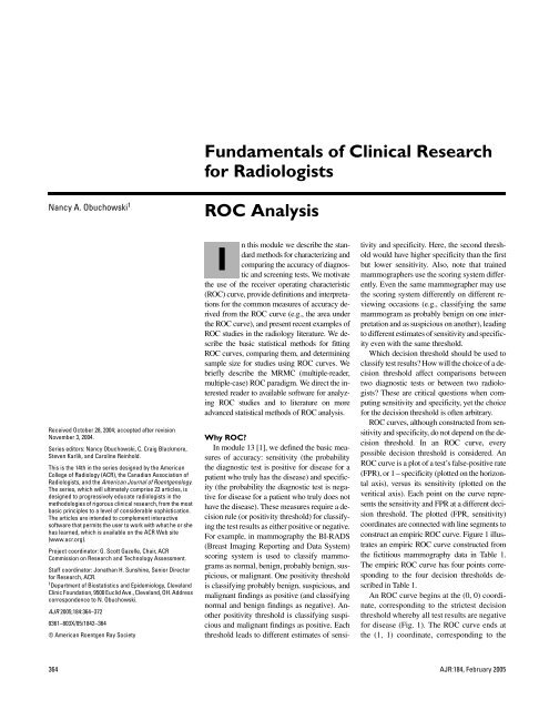
ROC Analysismost lenient decision threshold whereby alltest results are positive for disease. An empiricROC curve has h − 1 additional coordinates,where h is the number of unique testresults in the sample. In Table 1 there are 200test results, one for each of the 200 patients inthe sample, but there are only five unique results:normal, benign, probably benign, suspicious,and malignant. Thus, h = 5, and thereare four coordinates plotted in Figure 1 correspondingto the four decision thresholds describedin Table 1.The line connecting the (0, 0) and (1, 1)coordinates is called the “chance diagonal”and represents the ROC curve of a diagnostictest with no ability to distinguish patientswith versus those without disease. An ROCcurve that lies above the chance diagonal,such as the ROC curve for our fictitiousmammography example, has some diagnosticability. The further away an ROC curve isfrom the chance diagonal, and therefore, thecloser to the upper left-hand corner, the betterdiscriminating power and diagnostic accuracythe test has.In characterizing the accuracy of a diagnostic(or screening) test, the ROC curve ofthe test provides much more informationabout how the test performs than just a singleestimate of the test’s sensitivity and specificity[1, 2]. Given a test’s ROC curve, a cliniciancan examine the trade-offs in sensitivityversus specificity for various decision thresholds.Based on the relative costs of false-positiveand false-negative errors and the pretestprobability of disease, the clinician canchoose the optimal decision threshold foreach patient. This idea is discussed in moredetail in a later section of this article. Often,TABLE 1patient management is more complex than isallowed with a decision threshold that classifiesthe test results into positive or negative.For example, in mammography suspiciousand malignant findings are usually followedup with biopsy, probably benign findings usuallyresult in a follow-up mammogram in 3–6months, and normal and benign findings areconsidered negative.When comparing two or more diagnostictests, ROC curves are often the only validmethod of comparison. Figure 2 illustratestwo scenarios in which an investigator,comparing two diagnostic tests, could bemisled by relying on only a single sensitivity–specificity pair. Consider Figure 2A. Supposea more expensive or risky test (represented byROC curve Y) was reported to have thefollowing accuracy: sensitivity = 0.40,specificity = 0.90 (labeled as coordinate 1 inFig. 2A); a less expensive or less risky test(represented by ROC curve X) was reportedto have the following accuracy: sensitivity =0.80, specificity = 0.65 (labeled as coordinate2 in Fig. 2A). If the investigator is looking forthe test with better specificity, then he or shemay choose the more expensive, risky test,not realizing that a simple change in thedecision threshold of the less expensive,cheaper test could provide the desiredspecificity at an even higher sensitivity(coordinate 3 in Fig. 2A).Now consider Figure 2B. The ROC curvefor test Z is superior to that of test X for a narrowrange of FPRs (0.0–0.08); otherwise, diagnostictest X has superior accuracy. Acomparison of the tests’ sensitivities at lowFPRs would be misleading unless the diagnostictests are useful only at these low FPRs.Construction of Receiver Operating Characteristic Curve Based onFictitious Mammography DataMammography Results Pathology/Follow-Up Results Decision Rules 1–4(BI-RADs Score)Not Malignant Malignant FPR SensitivityNormal 65 5 (1) 35/100 95/100Benign 10 15 (2) 25/100 80/100Probably benign 15 10 (3) 10/100 70/100Suspicious 7 60 (4) 3/100 10/100Malignant 3 10Total 100 100Note.—Decision rule 1 classifies normal mammography findings as negative; all others are positive. Decision rule 2classifies normal and benign mammography findings as negative; all others are positive. Decision rule 3 classifies normal,benign, and probably benign findings as negative; all others are positive. Decision rule 4 classifies normal, benign,probably benign, and suspicious findings as negative; malignant is the only finding classified as positive. BI-RADS =Breast Imaging Reporting and Data System, FPR = false-positive rate.To compare two or more diagnostic tests, itis convenient to summarize the tests’ accuracieswith a single summary measure. Severalsuch summary measures are used in the literature.One is Youden’s index, defined as sensitivity+ specificity − 1 [2]. Note, however,that Youden’s index is affected by the choiceof the decision threshold used to define sensitivityand specificity. Thus, different decisionthresholds yield different values of theYouden’s index for the same diagnostic test.Another summary measure commonlyused is the probability of a correct diagnosis,often referred to simply as “accuracy” in theliterature. It can be shown that the probabilityof a correct diagnosis is equivalent toprobability (correct diagnosis) = PREV s ×sensitivity + (1 – PREV s ) × specificity, (1)where PREV s is the prevalence of disease inthe sample. That is, this summary measure ofaccuracy is affected not only by the choice ofthe decision threshold but also by the prevalenceof disease in the study sample [2]. Thus,even slight changes in the prevalence of diseasein the population of patients being testedcan lead to different values of “accuracy” forthe same test.Summary measures of accuracy derivedfrom the ROC curve describe the inherent accuracyof a diagnostic test because they are notaffected by the choice of the decision thresholdand they are not affected by the prevalence ofdisease in the study sample. Thus, these summarymeasures are preferable to Youden’s indexand the probability of a correct diagnosis[2]. The most popular summary measure of accuracyis the area under the ROC curve, oftendenoted as “AUC” for area under curve. Itranges in value from 0.5 (chance) to 1.0 (perfectdiscrimination or accuracy). The chancediagonal in Figure 1 has an AUC of 0.5. In Figure2A the areas under both ROC curves arethe same, 0.841. There are three interpretationsfor the AUC: the average sensitivity over allfalse-positive rates; the average specificityover all sensitivities [3]; and the probabilitythat, when presented with a randomly chosenpatient with disease and a randomly chosen patientwithout disease, the results of the diagnostictest will rank the patient with disease ashaving higher suspicion for disease than thepatient without disease [4].The AUC is often too global a summarymeasure. Instead, for a particular clinical application,a decision threshold is chosen sothat the diagnostic test will have a low FPRAJR:184, February 2005 365

Obuchowski(e.g., FPR < 0.10) or a high sensitivity (e.g.,sensitivity > 0.80). In these circumstances,the accuracy of the test at the specified FPRs(or specified sensitivities) is a more meaningfulsummary measure than the area under theentire ROC curve. The partial area under theROC curve, PAUC (e.g., the PAUC where FPR< 0.10, or the PAUC where sensitivity > 0.80),is then an appropriate summary measure of thediagnostic test’s accuracy. In Figure 2B, thePAUCs for the two tests where the FPR is between0.0 and 0.20 are the same, 0.112. Forinterpretation purposes, the PAUC is often dividedby its maximum value, given by therange (i.e., maximum–minimum) of the FPRs(or false-negative rates [FNRs]) [5]. ThePAUC divided by its maximum value is calledthe partial area index and takes on values between0.5 and 1.0, as does the AUC. It is interpretedas the average sensitivity for theFPRs examined (or average specificity for theFNRs examined). In our example, the rangeof the FPRs of interest is 0.20–0.0 = 0.20;thus, the average sensitivity for FPRs lessthan 0.20 for diagnostic tests X and Z in Figure2B is 0.56.Although the ROC curve has many advantagesin characterizing the accuracy of a diagnostictest, it also has some limitations. Onecriticism is that the ROC curve extends beyondthe clinically relevant area of potential clinicalinterpretation. Of course, the PAUC was developedto address this criticism. Another criticismis that it is possible for a diagnostic testwith perfect discrimination between diseasedand nondiseased patients to have an AUC of0.5. Hilden [6] describes this unusual situationand offers solutions. When comparing two diagnostictests’ accuracies, the tests’ ROCcurves can cross, as in Figure 2. A comparisonof these tests based only on their AUCs can bemisleading. Again, the PAUC attempts to addressthis limitation. Last, some [6, 7] criticizethe ROC curve, and especially the AUC, fornot incorporating the pretest probability of diseaseand the costs of misdiagnoses.Fig. 1.—Empiric and fitted (or “smooth”) receiver operatingcharacteristic (ROC) curves constructed frommammography data in Table 1. Four labeled points onempiric curve (dotted line) correspond to four decisionthresholds used to estimate sensitivity and specificity.Area under curve (AUC) for empiric ROC curve is 0.863and for fitted curve (solid line) is 0.876.and other relevant biases common to thesetypes of studies.In ROC studies we also require that the testresults, or the interpretations of the test images,be assigned a numeric value or rank. These numericmeasurements or ranks are the basis forSensitivity1.00.80.60.40.20.00.00.20.40.6False-Positive Rate0.81.0ASensitivity1.00.80.60.40.20.00.00.2Chance diagonal0.40.6False-Positive Rate0.81.0defining the decision thresholds that yield theestimates of sensitivity and specificity that areplotted to form the ROC curve. Some diagnostictests yield an objective measurement (e.g.,attenuation value of a lesion). The decisionthresholds for constructing the ROC curve areSensitivity1.00.80.60.40.20.00.00.20.40.6False-Positive RateFig. 2.—Two examples illustrate advantages of receiver operating characteristic (ROC) curves (see text for explanation)and comparing summary measures of accuracy.A, ROC curve Y (dotted line) has same area under curve (AUC) as ROC curve X (solid line), but lower partial areaunder curve (PAUC) when false-positive rate (FPR) is ≤ 0.20, and higher PAUC when false-positive rate > 0.20.B, ROC curve Z (dashed line) has same PAUC as curve X (solid line) when FPR ≤ 0.20 but lower AUC.1.00.81.0BThe ROC StudyWeinstein et al. [1] describe the commonfeatures of a study of the accuracy of a diagnostictest. These include samples from bothpatients with and those without the disease ofinterest and a reference standard for determiningwhether positive test results are truepositivesor false-positives, and whether negativetest results are true-negatives or falsenegatives.They also discuss the need to blindreviewers who are interpreting test imagesFig. 3.—Unobserved binormal distribution that wasassumed to underlie test results in Table 1. Distributionfor nondiseased patients was arbitrarily centeredat 0 with SD of 1 (i.e., µ o = 0 and σ o = 1). Binormal parameterswere estimated to be A = 2.27 and B = 1.70.Thus, distribution for diseased patients is centered atµ 1 = 1.335 with SD of σ 1 = 0.588. Four cutoffs, z1, z2, z3,and z4, correspond to four decision thresholds in Table1. If underlying test value is less than z1, then mammographerassigns test result of “normal." If theunderlying test value is less than z2 but greater thanz1, then mammographer assigns test result of “benign,”and so forth.Relative Frequency0.80.60.40.20.0DiseasedNondiseased-4 -2 0 2 4Unobserved Underlying Variable366 AJR:184, February 2005

ROC Analysisbased on increasing the values of the attenuationcoefficient. Other diagnostic tests must beinterpreted by a trained observer, often a radiologist,and so the interpretation is subjective.Two general scales are often used in radiologyfor observers to assign a value to their subjectiveinterpretation of an image. One scale is the5-point rank scale: 1 = definitely normal, 2 =probably normal, 3 = possibly abnormal orequivocal, 4 = probably abnormal, and 5 = definitelyabnormal.The other popular scale is the 0–100% confidencescale, where 0% implies that the observeris completely confident in the absenceof the disease of interest, and 100% impliesthat the observer is completely confident inthe presence of the disease of interest. Thetwo scales have strengths and weaknesses [2,8], but both are reasonably well suited to radiologyresearch. In mammography a ratingscale already exists, the BI-RADS score,which can be used to form decision thresholdsfrom least to most suspicion for the presenceof breast cancer.When the diagnostic test requires a subjectiveinterpretation by a trained reviewer, thereviewer becomes part of the diagnostic process[9]. Thus, to properly characterize the accuracyof the diagnostic test, we must includemultiple reviewers in the study. This is the socalledMRMC, multiple-reader multiplecase,ROC study. Much has been writtenabout the design and analysis of MRMC studies[10–20]. We mention here only the basicdesign of MRMC studies, and in a later subsectionwe describe their statistical analysis.The usual design for the MRMC study is afactorial design, in which every reviewer interpretsthe image (or images if there is morethan one test) of every patient. Thus, if thereare R reviewers, C patients, and I diagnostictests, then each reviewer interprets C × I images,and the study involves R × C × I total interpretations.The accuracy of each reviewerwith each diagnostic test is characterized byan ROC curve, so R × I ROC curves are constructed.Constructing pooled or consensusROC curves is not the goal of these studies.Rather, the primary goals are to document thevariability in diagnostic test accuracy betweenreviewers and report the average, ortypical, accuracy of reviewers. In order for theresults of the study to be generalizeable to therelevant patient and reviewer populations,representative samples from both populationsare needed for the study. Often expert reviewerstake part in studies of diagnostic test accuracy,but the accuracy for a nonexpert may beFig. 4.—Three receiver operating characteristic (ROC)curves with same binormal parameter A (i.e., A = 1.0)but different values for parameter B of 3.0 (3σ 1 = σ o ),1.0 (σ 1 = σ o ), and 0.33 (σ 1 = 3σ o ).When B = 3.0, ROCcurve dips below chance diagonal; this is called an improperROC curve [2].considerably less. An excellent illustration ofthe issues involved in sampling reviewers foran MRMC study can be found in the study byBeam et al. [21].Sensitivity1.00.80.60.40.20.00.0B = 3.3B = 1.00.2B = 3.00.40.6False-Positive Rate0.81.0Examples of ROC Studies in RadiologyThe radiology literature, and the clinicallaboratory and more general medical literature,contain many excellent examples of howROC curves are used to characterize the accuracyof a diagnostic test and to compare accuraciesof diagnostic tests. We briefly describehere three recent examples of ROC curves beingused in the radiology literature.Kim et al. [22] conducted a prospectivestudy to determine if rectal distention usingwarm water improves the accuracy of MRIfor preoperative staging of rectal cancer. AfterMRI, the patients underwent surgical resection,considered the gold standardregarding the invasion of adjacent structuresand regional lymph node involvement. Fourobservers, unaware of the pathology results,independently scored the MR images using 4-and 5-point rating scales. Using statisticalmethods for MRMC studies [13], the authorsdetermined that typical reviewers’ accuracyfor determining outer wall penetration is improvedwith rectum distention, but that revieweraccuracy for determining regionallymph node involvement is not affected.Osada et al. [23] used ROC analysis to assessthe ability of MRI to predict fetal pulmonaryhypoplasia. They imaged 87fetuses, measuring both lung volume andsignal intensity. An ROC curve based onlung volume showed that lung volume hassome ability to discriminate between fetuseswho will have good versus those who willhave poor respiratory outcome after birth.An ROC curve based on the combined informationfrom lung volume and signal intensity,however, has superior accuracy. Formore information on the optimal way tocombine measures or test results, see the articleby Pepe and Thompson [24].In a third study, Zheng et al. [25] assessedhow the accuracy of a mammographic computer-aideddetection (CAD) scheme wasaffected by restricting the maximum numberof regions that could be identified aspositive. Using a sample of 300 cases with amalignant mass and 200 normals, the investigatorsapplied their CAD system, each timereducing the maximum number of positiveregions that the CAD system could identifyfrom seven to one. A special ROC techniquecalled “free-response receiver operatingcharacteristic curves” (FROC) was used.The horizontal axis of the FROC curve differsfrom the traditional ROC curve in thatit gives the average number of false-positivesper image. Zheng et al. concluded thatlimiting the maximum number of positiveregions that the CAD could identify improvesthe overall accuracy of CAD in mammography.For more information on FROCcurves and related methods, I refer you toother articles [26–29].Statistical Methods for ROC AnalysisFitting Smooth ROC CurvesIn Figure 1 we saw the empiric ROC curvefor the test results in Table 1. The curve wasconstructed with line segments connectingthe observed points on the ROC curve. EmpiricROC curves often have a jagged appearance,as seen in Figure 1, and often lie slightlybelow the “true,” smooth, ROC curve—thatis, the test’s ROC curve if it were constructedwith an infinite number of points (not just thefour points in Fig. 1) and an infinitely largesample size. A smooth curve gives us a betteridea of the relationship between the diagnos-AJR:184, February 2005 367

Obuchowskitic test and the disease. In this subsection wedescribe some methods for constructingsmooth ROC curves.The most popular method of fitting asmooth ROC curve is to assume that the testresults (e.g., the BI-RADS scores in Table 1)come from two unobserved distributions, onedistribution for the patients with disease andone for the patients without the disease. Usuallyit is assumed that these two distributionscan be transformed to normal distributions,referred to as the binormal assumption. It isthe unobserved, underlying distributions thatwe assume can be transformed to follow abinormal distribution, and not the observedtest results. Figure 3 illustrates the hypothesizedunobserved binormal distribution estimatedfor the observed BI-RADS results inTable 1. Note how the distributions for thediseased and nondiseased patients overlap.Let the unobserved binormal variables forthe nondiseased and diseased patients havemeans µ 0 and µ 1 , and variances σ 0 [2] and σ 1[2], respectively. Then it can be shown [30]that the ROC curve is completed described bytwo parameters:A = (µ 1 – µ 0 ) / σ 1 (2)B = σ 0 / σ 1 . (3)(See Appendix 1 for a formula that linksparameters A and B to the ROC curve.) Figure4 illustrates three ROC curves. ParameterA was set to be constant at 1.0 and parameterB varies as follows: 0.33 (the underlying distributionof the diseased patients is threetimes more variable than that of the nondiseasedpatients), 1.0 (the two distributionshave the same SD), and 3.0 (the underlyingdistribution of the nondiseased patients isthree times more variable than that of the diseasedpatients). As one can see, the curvesdiffer dramatically with changes in parameterB. Parameter A, on the other hand, determineshow far the curve is above the chance diagonal(where A = 0); for a constant B parameter,the greater the value of A, the higher the ROCcurve lies (i.e., greater accuracy).Parameters A and B can be estimated fromdata such as in Table 1 using maximum likelihoodmethods [30, 31]. For the data in Table1, the maximum likelihood estimates (MLEs)of parameters A and B are 2.27 and 1.70, respectively;the smooth ROC curve is given inFigure 1. Fortunately, some useful software[32] has been written to perform the necessarycalculations of A and B, along with estimationof the area under the smooth curve(see next subsection), its SE and confidenceinterval (CI), and CIs for the ROC curve itself(see Appendix 1).Dorfman and Alf [30] suggested a statisticaltest to evaluate whether the binormal assumptionwas reasonable for a given data set. Others[33, 34] have shown through empiric investigationand simulation studies that many differentunderlying distributions are well approximatedby the binormal assumption.When the diagnostic test results are themselvesa continuous measurement (e.g., CTTABLE 2attenuation values, or measured lesion diameter),it may not be necessary to assume theexistence of an unobserved, underlying distribution.Sometimes continuous-scale testresults themselves follow a binormal distribution,but caution should be taken that thefit is good (see the article by Goddard andHinberg [35] for a discussion of the resultingbias when the distribution is not truly binormalyet the binormal distribution is assumed).Zou et al. [36] suggest using a Box-Cox transformation to transform data toEstimating Area Under Empirical Receiver Operating CharacteristicCurveTest ResultsScore xScore No. of PairsNondiseasedDiseasedNo. of PairsNormal Normal 1/2 65 x 5 = 325 162.5Normal Benign 1 65 x 15 = 975 975Normal Probably benign 1 65 x 10 = 650 650Normal Suspicious 1 65 x 60 = 3,900 3,900Normal Malignant 1 65 x 10 = 650 650Benign Normal 0 10 x 5 = 50 0Benign Benign 1/2 10 x 15 = 150 75Benign Probably benign 1 10 x 10 = 100 100Benign Suspicious 1 10 x 60 = 600 600Benign Malignant 1 10 x 10 = 100 100Probably benign Normal 0 15 x 5 = 75 0Probably benign Benign 0 15 x 15 = 225 0Probably benign Probably benign 1/2 15 x 10 = 150 75Probably benign Suspicious 1 15 x 60 = 900 900Probably benign Malignant 1 15 x 10 = 150 150Suspicious Normal 0 7 x 5 = 35 0Suspicious Benign 0 7 x 15 = 105 0Suspicious Probably benign 0 7 x 10 = 70 0Suspicious Suspicious 1/2 7 x 60 = 420 210Suspicious Malignant 1 7 x 10 = 70 70Malignant Normal 0 3 x 5 = 15 0Malignant Benign 0 3 x 15 = 45 0Malignant Probably benign 0 3 x 10 = 30 0Malignant Suspicious 0 3 x 60 = 180 0Malignant Malignant 1/2 3 x 10 = 30 15Total 10,000 pairs 8,632.5368 AJR:184, February 2005

ROC AnalysisTABLE 3 Fictitious Data Comparing the Accuracy of Two Diagnostic TestsROC CurveXYEstimated AUC 0.841 0.841Estimated SE of AUC 0.041 0.045Estimated PAUC where FPR < 0.20 0.112 0.071Estimated SE of PAUC 0.019 0.014Estimated covariance 0.00001Z test comparing PAUCs Z = [0.112 – 0.071] / √[0.019 2 + 0.014 2 – 0.00002]95% CI for difference in PAUCs [0.112 – 0.071] ± 1.96 × √[0.019 2 + 0.014 2 – 0.00002]Note.—AUC = area under the curve, PAUC = partial area under the curve, CI = confidence interval.binormality. Alternatively, one can use softwarelike ROCKIT [32] that will bin the testresults into an optimal number of categoriesand apply the same maximum likelihoodmethods as mentioned earlier for rating datalike the BI-RADS scores.More elaborate models for the ROC curve thatcan take into account covariates (e.g., the patient’sage, symptoms) have also been developedin the statistics literature [37–39] and will becomemore accessible as new software is written.Estimating the Area Under the ROC CurveEstimation of the area under the smoothcurve, assuming a binormal distribution, isdescribed in Appendix 1. In this subsection,we describe and illustrate estimation of thearea under the empiric ROC curve. The processof estimating the area under the empiricROC curve is nonparametric, meaning thatno assumptions are made about the distributionof the test results or about any hypothesizedunderlying distribution. The estimationworks for tests scored with a rating scale, a0–100% confidence scale, or a true continuous-scalevariable.The process of estimating the area under theempiric ROC curve involves four simple steps:First, the test result of a patient with disease iscompared with the test result of a patient withoutdisease. If the former test result indicatesmore suspicion of disease than the latter test result,then a score of 1 is assigned. If the test resultsare identical, then a score of 1/2 isassigned. If the diseased patient has a test resultindicating less suspicion for disease than thetest result of the nondiseased patient, then ascore of 0 is assigned. It does not matter whichdiseased and nondiseased patient you beginwith. Using the data in Table 1 as an illustration,suppose we start with a diseased patient assigneda test result of “normal” and a nondiseasedpatient assigned a test result of “normal.”Because their test results are the same, this pairis assigned a score of 1/2.Second, repeat the first step for every possiblepair of diseased and nondiseased patientsin your sample. In Table 1 there are 100diseased patients and 100 nondiseased patients,thus 10,000 possible pairs. Becausethere are only five unique test results, the10,000 possible pairs can be scored easily, asin Table 2.Third, sum the scores of all possible pairs.From Table 2, the sum is 8,632.5.Fourth, divide the sum from step 3 by thenumber of pairs in the study sample. In ourexample we have 10,000 pairs. Dividing thesum from step 3 by 10,000 gives us 0.86325,which is our estimate of the area under theempiric ROC curve. Note that this method ofestimating the area under the empiric ROCcurve gives the same result as one would obtainby fitting trapezoids under the curve andsumming the areas of the trapezoids (socalledtrapezoid method).The variance of the estimated area underthe empiric ROC curve is given by DeLonget al. [40] and can be used for constructingCIs; software programs are available for estimatingthe nonparametric AUC and itsvariance [41].Comparing the AUCs or PAUCs of TwoDiagnostic TestsTo test whether the AUC (or PAUC) of onediagnostic test (denoted by AUC 1 ) equals theAUC (or PAUC) of another diagnostic test(AUC 2 ), the following test statistic is calculated:Z = [AUC 1 – AUC 2 ] /√[var 1 + var 2 – 2 × cov], (4)where var 1 is the estimated variance of AUC 1 ,var 2 is the estimated variance of AUC 2 , andcov is the estimated covariance between AUC 1and AUC 2 . When different samples of patientsundergo the two diagnostic tests, the covarianceequals zero. When the same sample of patientsundergoes both diagnostic tests (i.e., a pairedstudy design), then the covariance is not generallyequal to zero and is often positive. The estimatedvariances and covariances are standardoutput for most ROC software [32, 41].The test statistic Z follows a standard normaldistribution. For a two-tailed test withsignificance level of 0.05, the critical valuesare –1.96 and +1.96. If Z is less than −1.96,then we conclude that the accuracy of diagnostictest 2 is superior to that of diagnostictest 1; if Z exceeds +1.96, then we concludethat the accuracy of diagnostic test 1 is superiorto that of diagnostic test 2.A two-sided CI for the difference in AUC(or PAUC) between two diagnostic tests canbe calculated fromLL = [AUC 1 – AUC 2 ] – z α/2 ×√[var 1 + var 2 – 2 × cov] (5)UL = [AUC 1 – AUC 2 ] + z α/2 ×√[var 1 + var 2 – 2 × cov], (6)where LL is the lower limit of the CI, UL isthe upper limit, and z α/2 is a value from thestandard normal distribution corresponding toa probability of α/2. For example, to constructa 95% CI, α = 0.05, thus z α/2 = 1.96.Consider the ROC curves in Figure 2A. Theestimated areas under the smooth ROC curves ofthe two tests are the same, 0.841. The PAUCswhere the FPR is greater than 0.20, however, differ.From the estimated variances and covariancein Table 3, the value of the Z statistic for comparingthe PAUCs is 1.77, which is not statisticallysignificant. The 95% CI for the difference inPAUCs is more informative: (−0.004 to 0.086);the CI for the partial area index is (−0.02 to 0.43).The CI contains large positive differences, suggestingthat more research is needed to investigatethe relative accuracies of these twodiagnostic tests for FPRs less than 0.20.Analysis of MRMC ROC StudiesMultiple published methods discuss performingthe statistical analysis of MRMC studies [13–20]. The methods are used to construct CIs for diagnosticaccuracy and statistical tests for assessingdifferences in accuracy between tests. Astatistical overview of the methods is given elsewhere[10]. Here, we briefly mention some of thekey issues of MRMC ROC analyses.AJR:184, February 2005 369

ObuchowskiFixed- or random-effects models.—TheMRMC study has two samples, a sample ofpatients and a sample of reviewers. If the studyresults are to be generalized to patients similarto ones in the study sample and to reviewerssimilar to ones in the study sample, then a statisticalanalysis that treats both patients and reviewersas random effects should be used [13,14, 17–20]. If the study results are to be generalizedto just patients similar to ones in thestudy sample, then the patients are treated asrandom effects but the reviewers should betreated as fixed effects [13–20]. Some of thestatistical methods can treat reviewers as eitherrandom or fixed, whereas other methodstreat reviewers only as fixed effects.Parametric or nonparametric.—Some of themethods rely on models that make strong assumptionsabout how the accuracies of the reviewersare correlated and distributed(parametric methods) [13, 14], other methods aremore flexible [15, 20], and still others make noassumptions [16–19] (nonparametric methods).The parametric methods may be more powerfulwhen their assumptions are met, but often it is difficultto determine if the assumptions are met.Covariates.—Reviewers’ accuracy may beaffected by their training or experience or bycharacteristics of the patients (e.g., age, sex,stage of disease, comorbidities). These variablesare called covariates. Some of the statisticalmethods [15, 20] have models that caninclude covariates. These models providevaluable insight into the variability betweenreviewers and between patients.Software.—Software is available for publicuse for some of the methods [32, 42, 43]; theauthors of the other methods may be able toprovide software if contacted.Determining Sample Size for ROC StudiesMany issues must be considered in determiningthe number of patients needed for anROC study. We list several of the key issuesand some useful references here, followed bya simple illustration. Software is also availablefor determining the required sample sizefor some ROC study designs [32, 41].1. Is it a MRMC ROC study? Many radiologystudies include more than one reviewerbut are not considered MRMC studies.MRMC studies usually involve five or more reviewersand focus on estimating the averageaccuracy of the reviewers. In contrast, many radiologystudies include two or three reviewersto get some idea of the interreviewer variability.Estimation of the required sample size forMRMC studies requires balancing the numberof reviewers in the reviewer sample with thenumber of patients in the patient sample. See[14, 44] for formulae for determining samplesizes for MRMC studies and [45] for samplesize tables for MRMC studies. Sample size determinationfor non-MRMC studies is basedon the number of patients needed.2. Will the study involve a single diagnostictest or compare two or morediagnostic tests? ROC studies comparingtwo or more diagnostic tests are common.These studies focus on the difference betweenAUCs or PAUCs of the two (or more)diagnostic tests. Sample size can be basedon either planning for enough statisticalpower to detect a clinically important difference,or constructing a CI for the differencein accuracies that is narrow enough to makeclinically relevant conclusions from thestudy. In studies of one diagnostic test, weoften focus on the magnitude of the test’sAUC or PAUC, basing sample size on thedesired width of a CI.3. If two or more diagnostic tests arebeing compared, will it be a paired orunpaired study design, and are the accuraciesof the tests hypothesized to bedifferent or equivalent? Paired designsalmost always require fewer patients than anunpaired design, and so are used wheneverthey are logistically, ethically, and financiallyfeasible. Studies that are performed to determinewhether two or more tests have the sameaccuracy are called equivalency studies. Oftenin radiology a less invasive diagnostic test,or a quicker imaging sequence, is developedand compared with the standard test. The investigatorwants to know if the test is similarin accuracy to the standard test. Equivalencystudies often require a larger sample size thanstudies in which the goal is to show that onetest has superior accuracy to another test. Thereason is that to show equivalence the investigatormust rule out all large differences betweenthe tests—that is, the CI for thedifference must be very narrow.4. Will the patients be recruited in aprospective or retrospective fashion?In prospective designs, patients are recruitedbased on their signs or symptoms, so at thetime of recruitment it is unknown whether thepatient has the disease of interest. In contrast,in retrospective designs patients are recruitedbased on their known true disease status (asdetermined by the gold or reference standard)[2]. Both studies are used commonly in radiology.Retrospective studies often requirefewer patients than prospective designs.5. What will be the ratio of nondiseasedto diseased patients in thestudy sample? Let k denote the ratio ofthe number of nondiseased to diseased patientsin the study sample. For retrospectivestudies k is usually decided in the designphase of the study. For prospective designsk is unknown in the design phase but can beestimated by (1 – PREV p ) / PREV p , wherePREV p is the prevalence of disease in therelevant population. A range of values for-PREV p should be considered when determiningsample size.6. What summary measure of accuracywill be used? In this article we havefocused mainly on the AUC and PAUC, butothers are possible (see [2]). The choice ofsummary measures determines which variancefunction formula will be used in calculatingsample size. Note that the variancefunction is related to the variance by the followingformula: variance = VF / N, where VFis the variance function and N is the numberof study patients with disease.7. What is the conjectured accuracyof the diagnostic test? The conjectured accuracyis needed to determine the expecteddifference in accuracy between two or morediagnostic tests. Also, the magnitude of theaccuracy affects the variance function. In thefollowing example, we present the variancefunction for the AUC; see Zhou et al. [2] forformulae for other variance functions.Consider the following example. Supposean investigator wants to conduct a study to determineif MRI can distinguish benign frommalignant breast lesions. Patients with a suspiciouslesion detected on mammography will beprospectively recruited to undergo MRI beforebiopsy. The pathology results will be the referencestandard. The MR images will be interpretedindependently by two reviewers; theywill score the lesions using a 0–100% confidencescale. An ROC curve will be constructedfor each reviewer; AUCs will be estimated, and95% CIs for the AUCs will be constructed. IfMRI shows some promise, the investigator willplan a larger MRMC study.The investigator expects 20–40% of patientsto have pathologically confirmed breast cancer(PREV p = 0.2–0.4); thus, k = 1.5–4.0. The investigatorexpects the AUC of MRI to be approximately0.80 or higher. The variancefunction of the AUC often used for sample sizecalculations is as follows:VF = (0.0099 × e –A×A/2 ) ×[(5 × A 2 + 8) + (A 2 + 8) / k], (7)370 AJR:184, February 2005

ROC Analysiswhere A is the parameter from the binormaldistribution. Parameter A can be calculatedfrom A = φ −1 (AUC) × 1.414, where φ −1 is the inverseof the cumulative normal distribution function[2]. For our example, AUC = 0.80; thusφ −1 (0.80) = 0.84 and A = 1.18776. The variancefunction, VF, equals (0.00489) × [(15.05387) +(9.41077) / 4.0] = 0.08512, where we have set k= 4.0. For k = 1.5, the VF = 0.10429.Suppose the investigator wants a 95% CIno wider than 0.10. That is, if the estimatedAUC from the study is 0.80, then the lowerbound of the CI should not be less than 0.75and the upper bound should not exceed 0.85.A formula for calculating the required samplesize for a CI isN = [z α/22× VF] / L 2 (8)where z α/2 = 1.96 for a 95% CI and L is thedesired half-width of the CI. Here, L = 0.05.N is the number of patients with diseaseneeded for the study; the total number of patientsneeded for the study is N × (1 + k). Forour example, N equals [1.96 2 × 0.08512] /0.05 2 = 130.8 for k = 4.0, and 160.3 for k =1.5. Thus, depending on the unknown prevalenceof breast cancer in the study sample, theinvestigator needs to recruit perhaps as few as401 total patients (if the sample prevalence is40%) but perhaps as many as 654 (if the sampleprevalence is only 20%).Finding the Optimal Point on the CurveMetz [46] derived a formula for determiningthe optimal decision threshold on the ROCcurve, where “optimal” is in terms of minimizingthe overall costs. “Costs” can be defined asmonetary costs, patient morbidity and mortality,or both. The slope, m, of the ROC curve atthe optimal decision threshold ism = (1 – PREV p ) / PREV p ×[C FP – C TN ] / [C FN – C TP ] (9)where C FP , C TN , C FN , and C TP are the costs offalse-positive, true-negative, false-negative, andtrue-positive results, respectively. Once m is estimated,the optimal decision threshold is theone for which sensitivity and specificity maximizethe following expression: [sensitivity –m(1 – specificity)] [47].Examining the ROC curve labeled X inFigure 2, we see that the slope is very steep inthe lower left where both the sensitivity andFPR are low, and is close to zero at the upperright where the sensitivity and FPR are high.The slope takes on a high value when the patientis unlikely to have the disease or the costof a false-positive is large; for these situations,a low FPR is optimal. The slope takeson a value near zero when the patient is likelyto have the disease or treatment for the diseaseis beneficial and carries little risk tohealthy patients; in these situations, a highsensitivity is optimal [3]. A nice example of astudy using this equation is given in [48]. Seealso work by Greenhouse and Mantel [49]and Linnet [50] for determining the optimaldecision threshold when a desired level forthe sensitivity, specificity, or both is specifieda priori.ConclusionApplications of ROC curves in the medicalliterature have increased greatly in thepast few decades, and with this expansionmany new statistical methods of ROC analysishave been developed. These includemethods that correct for common biases likeverification bias and imperfect gold standardbias, methods for combining the informationfrom multiple diagnostic tests (i.e., optimalcombinations of tests) and multiple studies(i.e., meta-analysis), and methods for analyzingclustered data (i.e., multiple observationsfrom the same patient). Interested readers cansearch directly for these statistical methods orconsult two recently published books on ROCcurve analysis and related topics [2, 39].Available software for ROC analysis allowsinvestigators to easily fit, evaluate, and compareROC curves [41, 51], although usersshould be cautious about the validity of thesoftware and check the underlying methodsand assumptions.AcknowledgmentsI thank the two series’ coeditors and an outsidestatistician for their helpful comments onan earlier draft of this manuscript.References1. Weinstein S, Obuchowski NA, Lieber ML. Clinicalevaluation of diagnostic tests. AJR2005;184:14–192. Zhou XH, Obuchowski NA, McClish DK. Statisticalmethods in diagnostic medicine. New York,NY: Wiley-Interscience, 20023. Metz CE. Some practical issues of experimentaldesign and data analysis in radiologic ROC studies.Invest Radiol 1989;24:234–2454. Hanley JA, McNeil BJ. The meaning and use ofthe area under a receiver operating characteristic(ROC) curve. Radiology 1982;143:29–365. McClish DK. Analyzing a portion of the ROCcurve. Med Decis Making 1989;9:190–1956. Hilden J. The area under the ROC curve and itscompetitors. Med Decis Making 1991;11:95–1017. Hilden J. Prevalence-free utility-respecting summaryindices of diagnostic power do not exist. StatMed 2000;19:431–4408. Wagner RF, Beiden SV, Metz CE. Continuous versuscategorical data for ROC analysis: some quantitativeconsiderations. Acad Radiol 2001;8:328–3349. Beam CA, Baker ME, Paine SS, Sostman HD, SullivanDC. Answering unanswered questions: proposalfor a shared resource in clinical diagnosticradiology research. Radiology 1992;183:619–62010. Obuchowski NA, Beiden SV, Berbaum KS, et al.Multireader multicase receiver operating characteristicanalysis: an empirical comparison of fivemethods. Acad Radiol 2004;11:980–99511. Obuchowski NA. Multi-reader ROC studies: acomparison of study designs. Acad Radiol1995;2:709–71612. Roe CA, Metz CE. Variance-component modelingin the analysis of receiver operating characteristic indexestimates. Acad Radiol 1997;4:587–60013. Dorfman DD, Berbaum KS, Metz CE. Receiver operatingcharacteristic rating analysis: generalizationto the population of readers and patients with thejackknife method. Invest Radiol 1992;27:723–73114. Obuchowski NA. Multi-reader multi-modalityROC studies: hypothesis testing and sample sizeestimation using an ANOVA approach with dependentobservations. with rejoinder. Acad Radiol1995;2:S22–S2915. Toledano AY, Gatsonis C. Ordinal regressionmethodology for ROC curves derived from correlateddata. Stat Med 1996;15:1807–182616. Song HH. Analysis of correlated ROC areas in diagnostictesting. Biometrics 1997;53:370–38217. Beiden SV, Wagner RF, Campbell G. Components-of-variancemodels and multiple-bootstrapexperiments: an alternative method for randomeffects,receiver operating characteristic analysis.Acad Radiol 2000;7:341–34918. Beiden SV, Wagner RF, Campbell G, Metz CE, JiangY. Components-of-variance models for random-effectsROC analysis: the case of unequal variance structureacross modalities. Acad Radiol 2001;8:605–61519. Beiden SV, Wagner RF, Campbell G, Chan HP.Analysis of uncertainties in estimates of componentsof variance in multivariate ROC analysis.Acad Radiol 2001;8:616–62220. Ishwaran H, Gatsonis CA. A general class of hierarchicalordinal regression models with applicationsto correlated ROC analysis. Can J Stat2000;28:731–75021. Beam CA, Layde PM, Sullivan DC. Variability inthe interpretation of screening mammograms byUS radiologists: findings from a national sample.Arch Intern Med 1996;156:209–21322. Kim MJ, Lim JS, Oh YT, et al. Preoperative MRI ofrectal cancer with and without rectal water filling: an intraindividualcomparison. AJR 2004;182:1469–147623. Osada H, Kaku K, Masuda K, Iitsuka Y, Seki K,Sekiya S. Quantitative and qualitative evaluationsof fetal lung with MR imaging. Radiology2004;231:887–89224. Pepe MS, Thompson ML. Combining diagnostictest results to increase accuracy. Biostatistics2000;1:123–140AJR:184, February 2005 371

Obuchowski25. Zheng B, Leader JK, Abrams G, et al. Computeraideddetection schemes: the effect of limiting thenumber of cued regions in each case. AJR2004;182:579–58326. Chakraborty DP, Winter LHL. Free-response methodology:alternative analysis and a new observer-performanceexperiment. Radiology 1990;174:873–88127. Chakraborty DP. Maximum likelihood analysis offree-response receiver operating characteristic(FROC) data. Med Phys 1989;16:561–56828. Swensson RG. Unified measurement of observerperformance in detecting and localizing target objectson images. Med Phys 1996;23:1709–172529. Obuchowski NA, Lieber ML, Powell KA. Dataanalysis for detection and localization of multipleabnormalities with application to mammography.Acad Radiol 2000;7:516–52530. Dorfman DD, Alf E. Maximum likelihood estimationof parameters of signal detection theory: adirect solution. Psychometrika 1968;33:117–12431. Dorfman DD, Alf E. Maximum-likelihood estimationof parameters of signal detection theoryand determination of confidence intervals: ratingmethod data. J Math Psychol 1969;6:487–49632. ROCKIT and LABMRMC. Available at:xray.bsd.uchicago.edu/krl/KRL_ROCsoftware_index.htm. Accessed December 13, 200433. Swets JA. Empirical RO. Cs in discrimination and diagnostictasks: implications for theory and measurementof performance. Psychol Bull 1986;99:181–19834. Hanley JA. The robustness of the binormal assumptionused in fitting ROC curves. Med DecisMaking 1988;8:197–20335. Goddard MJ, Hinberg I. Receiver operating characteristic(ROC) curves and non-normal data: anempirical study. Stat Med 1990;9:325–33736. Zou KH, Tempany CM, Fielding JR, Silverman SG.Original smooth receiver operating characteristiccurve estimation from continuous data: statisticalmethods for analyzing the predictive value of spiralCT of ureteral stones. Acad Radiol 1998;5:680–68737. Pepe MS. A regression modeling framework for receiveroperating characteristic curves in medical diagnostictesting. Biometrika 1997;84:595–60838. Pepe MS. An interpretation for the ROC curve usingGLM procedures. Biometrics 2000;56:352–35939. Pepe MS. The statistical evaluation of medicaltests for classification and prediction. New York,NY: Oxford University Press, 200340. DeLong ER, DeLong DM, Clarke-Pearson DL.Comparing the areas under two or more correlated receiveroperating characteristic curves: a nonparametricapproach. Biometrics 1988;44:837–84441. ROC analysis. Available at: www.bio.ri.ccf.org/Research/ROC/index.html. Accessed December13, 200442. OBUMRM. Available at: www.bio.ri.ccf.org/OBUMRM/OBUMRM.html. Accessed December13, 200443. The University of Iowa Department of Radiology:The Medical Image Perception Laboratory.MRMC 2.0. Available at: perception.radiology.uiowa.edu.Accessed December 13, 200444. Hillis SL, Berbaum KS. Power estimation for the Dorfman-Berbaum-Metzmethod. Acad Radiol (in press)45. Obuchowski NA. Sample size tables for receiver operatingcharacteristic studies. AJR 2000;175:603–60846. Metz CE. Basic principles of ROC analysis.Semin Nucl Med 1978;8:283–29847. Zweig MH, Campbell G. Receiver-operating characteristic(ROC) plots: a fundamental evaluation toolin clinical medicine. Clin Chem 1993;39:561–57748. Somoza E, Mossman D. “Biological markers” andpsychiatric diagnosis: risk-benefit balancing usingROC analysis. Biol Psychiatry 1991;29:811–82649. Greenhouse SW, Mantel N. The evaluation of diagnostictests. Biometrics 1950;6:399–41250. Linnet K. Comparison of quantitative diagnostictests: type I error, power, and sample size. StatMed 1987;6:147–15851. Stephan C, Wesseling S, Schink T, Jung K. Comparisonof eight computer programs for receiveroperatingcharacteristic analysis. Clin Chem2003;49:433–43952. Ma G, Hall WJ. Confidence bands for receiver operatingcharacteristic curves. Med Decis Making1993;13:191–197APPENDIX 1. Area Under the Curve and Confidence Intervals with Binormal ModelUnder the binormal assumption, the receiver operating characteristic (ROC) curve is thecollection of points given by[1 – φ(c), 1 – φ(B × c – A)]where c ranges from –∞ to +∞ and represents all the possible values of the underlying binormaldistribution, and φ is the cumulative normal distribution evaluated at c. For example, for a falsepositiverate of 0.10, φ(c) is set equal to 0.90; from tables of the cumulative normal distribution,we have φ(1.28) = 0.90. Suppose A = 2.0 and B = 1.0; then the sensitivity = 1 – φ(− 0.72) = 1 –0.2358 = 0.7642.ROCKIT [32] gives a confidence interval (CI) for sensitivity at particular false-positiverates (i.e., pointwise CIs). A CI for the entire ROC curve (i.e., simultaneous CI) is describedby Ma and Hall [52].Under the binormal distribution assumption, the area under the smooth ROC curve (AUC)is given byAUC = φ[A / √ (1 + B 2 )].For the example above, AUC = φ[2.0 / √ (2.0)] = φ[1.414] = 0.921.The variance of the full area under the ROC curve is given as standard output in programs likeROCKIT [32]. An estimator for the variance of the partial area under the curve (PAUC) was givenby McClish [5]; a Fortran program is available for estimating the PAUC and its variance [41].The reader’s attention is directed to earlier articles in the Fundamentals of Clinical Research series:1. Introduction, which appeared in February 20012. The Research Framework, April 20013. Protocol, June 20014. Data Collection, October 20015. Population and Sample, November 20016. Statistically Engineering the Study for Success, July 20027. Screening for Preclinical Disease: Test and DiseaseCharacteristics, October 20028. Exploring and Summarizing Radiologic Data, January 20039. Visualizing Radiologic Data, March 200310. Introduction to Probability Theory and SamplingDistributions, April 200311. Observational Studies in Radiology, November 200412. Randomized Controlled Trials, December 200413. Clinical Evaluation of Diagnostic Tests, January 2005372 AJR:184, February 2005