Fundamentals of Clinical Research for Radiologists ROC Analysis

More documents

Recommendations

Info

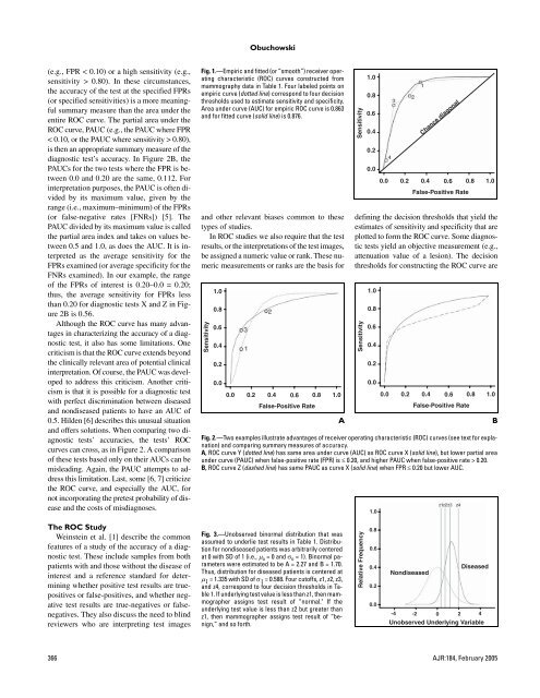
ROC Analysismost lenient decision threshold whereby alltest results are positive for disease. An empiricROC curve has h − 1 additional coordinates,where h is the number of unique testresults in the sample. In Table 1 there are 200test results, one for each of the 200 patients inthe sample, but there are only five unique results:normal, benign, probably benign, suspicious,and malignant. Thus, h = 5, and thereare four coordinates plotted in Figure 1 correspondingto the four decision thresholds describedin Table 1.The line connecting the (0, 0) and (1, 1)coordinates is called the “chance diagonal”and represents the ROC curve of a diagnostictest with no ability to distinguish patientswith versus those without disease. An ROCcurve that lies above the chance diagonal,such as the ROC curve for our fictitiousmammography example, has some diagnosticability. The further away an ROC curve isfrom the chance diagonal, and therefore, thecloser to the upper left-hand corner, the betterdiscriminating power and diagnostic accuracythe test has.In characterizing the accuracy of a diagnostic(or screening) test, the ROC curve ofthe test provides much more informationabout how the test performs than just a singleestimate of the test’s sensitivity and specificity[1, 2]. Given a test’s ROC curve, a cliniciancan examine the trade-offs in sensitivityversus specificity for various decision thresholds.Based on the relative costs of false-positiveand false-negative errors and the pretestprobability of disease, the clinician canchoose the optimal decision threshold foreach patient. This idea is discussed in moredetail in a later section of this article. Often,TABLE 1patient management is more complex than isallowed with a decision threshold that classifiesthe test results into positive or negative.For example, in mammography suspiciousand malignant findings are usually followedup with biopsy, probably benign findings usuallyresult in a follow-up mammogram in 3–6months, and normal and benign findings areconsidered negative.When comparing two or more diagnostictests, ROC curves are often the only validmethod of comparison. Figure 2 illustratestwo scenarios in which an investigator,comparing two diagnostic tests, could bemisled by relying on only a single sensitivity–specificity pair. Consider Figure 2A. Supposea more expensive or risky test (represented byROC curve Y) was reported to have thefollowing accuracy: sensitivity = 0.40,specificity = 0.90 (labeled as coordinate 1 inFig. 2A); a less expensive or less risky test(represented by ROC curve X) was reportedto have the following accuracy: sensitivity =0.80, specificity = 0.65 (labeled as coordinate2 in Fig. 2A). If the investigator is looking forthe test with better specificity, then he or shemay choose the more expensive, risky test,not realizing that a simple change in thedecision threshold of the less expensive,cheaper test could provide the desiredspecificity at an even higher sensitivity(coordinate 3 in Fig. 2A).Now consider Figure 2B. The ROC curvefor test Z is superior to that of test X for a narrowrange of FPRs (0.0–0.08); otherwise, diagnostictest X has superior accuracy. Acomparison of the tests’ sensitivities at lowFPRs would be misleading unless the diagnostictests are useful only at these low FPRs.Construction of Receiver Operating Characteristic Curve Based onFictitious Mammography DataMammography Results Pathology/Follow-Up Results Decision Rules 1–4(BI-RADs Score)Not Malignant Malignant FPR SensitivityNormal 65 5 (1) 35/100 95/100Benign 10 15 (2) 25/100 80/100Probably benign 15 10 (3) 10/100 70/100Suspicious 7 60 (4) 3/100 10/100Malignant 3 10Total 100 100Note.—Decision rule 1 classifies normal mammography findings as negative; all others are positive. Decision rule 2classifies normal and benign mammography findings as negative; all others are positive. Decision rule 3 classifies normal,benign, and probably benign findings as negative; all others are positive. Decision rule 4 classifies normal, benign,probably benign, and suspicious findings as negative; malignant is the only finding classified as positive. BI-RADS =Breast Imaging Reporting and Data System, FPR = false-positive rate.To compare two or more diagnostic tests, itis convenient to summarize the tests’ accuracieswith a single summary measure. Severalsuch summary measures are used in the literature.One is Youden’s index, defined as sensitivity+ specificity − 1 [2]. Note, however,that Youden’s index is affected by the choiceof the decision threshold used to define sensitivityand specificity. Thus, different decisionthresholds yield different values of theYouden’s index for the same diagnostic test.Another summary measure commonlyused is the probability of a correct diagnosis,often referred to simply as “accuracy” in theliterature. It can be shown that the probabilityof a correct diagnosis is equivalent toprobability (correct diagnosis) = PREV s ×sensitivity + (1 – PREV s ) × specificity, (1)where PREV s is the prevalence of disease inthe sample. That is, this summary measure ofaccuracy is affected not only by the choice ofthe decision threshold but also by the prevalenceof disease in the study sample [2]. Thus,even slight changes in the prevalence of diseasein the population of patients being testedcan lead to different values of “accuracy” forthe same test.Summary measures of accuracy derivedfrom the ROC curve describe the inherent accuracyof a diagnostic test because they are notaffected by the choice of the decision thresholdand they are not affected by the prevalence ofdisease in the study sample. Thus, these summarymeasures are preferable to Youden’s indexand the probability of a correct diagnosis[2]. The most popular summary measure of accuracyis the area under the ROC curve, oftendenoted as “AUC” for area under curve. Itranges in value from 0.5 (chance) to 1.0 (perfectdiscrimination or accuracy). The chancediagonal in Figure 1 has an AUC of 0.5. In Figure2A the areas under both ROC curves arethe same, 0.841. There are three interpretationsfor the AUC: the average sensitivity over allfalse-positive rates; the average specificityover all sensitivities [3]; and the probabilitythat, when presented with a randomly chosenpatient with disease and a randomly chosen patientwithout disease, the results of the diagnostictest will rank the patient with disease ashaving higher suspicion for disease than thepatient without disease [4].The AUC is often too global a summarymeasure. Instead, for a particular clinical application,a decision threshold is chosen sothat the diagnostic test will have a low FPRAJR:184, February 2005 365
Obuchowski(e.g., FPR < 0.10) or a high sensitivity (e.g.,sensitivity > 0.80). In these circumstances,the accuracy of the test at the specified FPRs(or specified sensitivities) is a more meaningfulsummary measure than the area under theentire ROC curve. The partial area under theROC curve, PAUC (e.g., the PAUC where FPR< 0.10, or the PAUC where sensitivity > 0.80),is then an appropriate summary measure of thediagnostic test’s accuracy. In Figure 2B, thePAUCs for the two tests where the FPR is between0.0 and 0.20 are the same, 0.112. Forinterpretation purposes, the PAUC is often dividedby its maximum value, given by therange (i.e., maximum–minimum) of the FPRs(or false-negative rates [FNRs]) [5]. ThePAUC divided by its maximum value is calledthe partial area index and takes on values between0.5 and 1.0, as does the AUC. It is interpretedas the average sensitivity for theFPRs examined (or average specificity for theFNRs examined). In our example, the rangeof the FPRs of interest is 0.20–0.0 = 0.20;thus, the average sensitivity for FPRs lessthan 0.20 for diagnostic tests X and Z in Figure2B is 0.56.Although the ROC curve has many advantagesin characterizing the accuracy of a diagnostictest, it also has some limitations. Onecriticism is that the ROC curve extends beyondthe clinically relevant area of potential clinicalinterpretation. Of course, the PAUC was developedto address this criticism. Another criticismis that it is possible for a diagnostic testwith perfect discrimination between diseasedand nondiseased patients to have an AUC of0.5. Hilden [6] describes this unusual situationand offers solutions. When comparing two diagnostictests’ accuracies, the tests’ ROCcurves can cross, as in Figure 2. A comparisonof these tests based only on their AUCs can bemisleading. Again, the PAUC attempts to addressthis limitation. Last, some [6, 7] criticizethe ROC curve, and especially the AUC, fornot incorporating the pretest probability of diseaseand the costs of misdiagnoses.Fig. 1.—Empiric and fitted (or “smooth”) receiver operatingcharacteristic (ROC) curves constructed frommammography data in Table 1. Four labeled points onempiric curve (dotted line) correspond to four decisionthresholds used to estimate sensitivity and specificity.Area under curve (AUC) for empiric ROC curve is 0.863and for fitted curve (solid line) is 0.876.and other relevant biases common to thesetypes of studies.In ROC studies we also require that the testresults, or the interpretations of the test images,be assigned a numeric value or rank. These numericmeasurements or ranks are the basis forSensitivity1.00.80.60.40.20.00.00.20.40.6False-Positive Rate0.81.0ASensitivity1.00.80.60.40.20.00.00.2Chance diagonal0.40.6False-Positive Rate0.81.0defining the decision thresholds that yield theestimates of sensitivity and specificity that areplotted to form the ROC curve. Some diagnostictests yield an objective measurement (e.g.,attenuation value of a lesion). The decisionthresholds for constructing the ROC curve areSensitivity1.00.80.60.40.20.00.00.20.40.6False-Positive RateFig. 2.—Two examples illustrate advantages of receiver operating characteristic (ROC) curves (see text for explanation)and comparing summary measures of accuracy.A, ROC curve Y (dotted line) has same area under curve (AUC) as ROC curve X (solid line), but lower partial areaunder curve (PAUC) when false-positive rate (FPR) is ≤ 0.20, and higher PAUC when false-positive rate > 0.20.B, ROC curve Z (dashed line) has same PAUC as curve X (solid line) when FPR ≤ 0.20 but lower AUC.1.00.81.0BThe ROC StudyWeinstein et al. [1] describe the commonfeatures of a study of the accuracy of a diagnostictest. These include samples from bothpatients with and those without the disease ofinterest and a reference standard for determiningwhether positive test results are truepositivesor false-positives, and whether negativetest results are true-negatives or falsenegatives.They also discuss the need to blindreviewers who are interpreting test imagesFig. 3.—Unobserved binormal distribution that wasassumed to underlie test results in Table 1. Distributionfor nondiseased patients was arbitrarily centeredat 0 with SD of 1 (i.e., µ o = 0 and σ o = 1). Binormal parameterswere estimated to be A = 2.27 and B = 1.70.Thus, distribution for diseased patients is centered atµ 1 = 1.335 with SD of σ 1 = 0.588. Four cutoffs, z1, z2, z3,and z4, correspond to four decision thresholds in Table1. If underlying test value is less than z1, then mammographerassigns test result of “normal." If theunderlying test value is less than z2 but greater thanz1, then mammographer assigns test result of “benign,”and so forth.Relative Frequency0.80.60.40.20.0DiseasedNondiseased-4 -2 0 2 4Unobserved Underlying Variable366 AJR:184, February 2005
Page 4 and 5: ROC Analysisbased on increasing the
Page 6 and 7: ROC AnalysisTABLE 3 Fictitious Data
Page 8 and 9: ROC Analysiswhere A is the paramete

Fundamentals of Clinical Research for Radiologists ROC Analysis

You also want an ePaper? Increase the reach of your titles

Delete template?

Save as template?