MATH 590: Meshfree Methods - Chapter 8 - Illinois Institute of ...

MATH 590: Meshfree MethodsChapter 8: Examples of Conditionally Positive Definite FunctionsGreg FasshauerDepartment of Applied MathematicsIllinois Institute of TechnologyFall 2010fasshauer@iit.edu MATH 590 – Chapter 8 1

Outline1 Example 1: Generalized Multiquadrics2 Example 2: Radial Powers3 Example 3: Thin Plate Splinesfasshauer@iit.edu MATH 590 – Chapter 8 2

We present some strictly conditionally positive definite (radial)functions that are covered by the Fourier transformcharacterization theorem of the previous chapter.fasshauer@iit.edu MATH 590 – Chapter 8 3

We present some strictly conditionally positive definite (radial)functions that are covered by the Fourier transformcharacterization theorem of the previous chapter.The generalized Fourier transforms for these examples areexplicitly computed in [Wendland (2005a)].fasshauer@iit.edu MATH 590 – Chapter 8 3

We present some strictly conditionally positive definite (radial)functions that are covered by the Fourier transformcharacterization theorem of the previous chapter.The generalized Fourier transforms for these examples areexplicitly computed in [Wendland (2005a)].Instead of going through these complicated calculations we willestablish the strict conditional positive definiteness of thesefunctions in the next chapter with the help of completely monotonefunctions.fasshauer@iit.edu MATH 590 – Chapter 8 3

We present some strictly conditionally positive definite (radial)functions that are covered by the Fourier transformcharacterization theorem of the previous chapter.The generalized Fourier transforms for these examples areexplicitly computed in [Wendland (2005a)].Instead of going through these complicated calculations we willestablish the strict conditional positive definiteness of thesefunctions in the next chapter with the help of completely monotonefunctions.The examples include some of the best known radial basicfunctions such asthe multiquadric due to [Hardy (1971)],and the thin plate spline due to [Duchon (1976)].fasshauer@iit.edu MATH 590 – Chapter 8 3

OutlineExample 1: Generalized Multiquadrics1 Example 1: Generalized Multiquadrics2 Example 2: Radial Powers3 Example 3: Thin Plate Splinesfasshauer@iit.edu MATH 590 – Chapter 8 4

Example 1: Generalized MultiquadricsGeneralized multiquadricΦ(x) = (1 + ‖x‖ 2 ) β , x ∈ R s , β ∈ R \ N 0 (1)fasshauer@iit.edu MATH 590 – Chapter 8 5

Example 1: Generalized MultiquadricsGeneralized multiquadricΦ(x) = (1 + ‖x‖ 2 ) β , x ∈ R s , β ∈ R \ N 0 (1)Generalized Fourier transformˆΦ(ω) = 21+βΓ(−β) ‖ω‖−β−s/2 K β+s/2 (‖ω‖), ω ≠ 0,of order m = max(0, ⌈β⌉).HereRemark⌈β⌉: smallest integer ≥ β,K ν : modified Bessel functions of the second kind of order νWe need to exclude β ∈ N 0 since this would lead to polynomials ofeven degree (see the related discussion in Example 2 and in HW 1).fasshauer@iit.edu MATH 590 – Chapter 8 5

Example 1: Generalized MultiquadricsSince the generalized Fourier transforms are positive with a singularityof order m at the origin, the FT characterization theorem from theprevious chapter tells us that the functionsΦ(x) = (−1) ⌈β⌉ (1 + ‖x‖ 2 ) β , 0 < β /∈ N,are strictly conditionally positive definite of order m = ⌈β⌉ (and higher).fasshauer@iit.edu MATH 590 – Chapter 8 6

Example 1: Generalized MultiquadricsSince the generalized Fourier transforms are positive with a singularityof order m at the origin, the FT characterization theorem from theprevious chapter tells us that the functionsΦ(x) = (−1) ⌈β⌉ (1 + ‖x‖ 2 ) β , 0 < β /∈ N,are strictly conditionally positive definite of order m = ⌈β⌉ (and higher).RemarkFor β < 0 the Fourier transform is a classical one and we are back tothe generalized inverse multiquadrics of Chapter 4.These functions are again shown to be strictly conditionally positivedefinite of order m = 0, i.e., strictly positive definite.fasshauer@iit.edu MATH 590 – Chapter 8 6

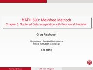
Example 1: Generalized MultiquadricsFigure: Hardy’s multiquadric with β = 1 2(left) and a generalized multiquadricwith β = 5 2 (right) centered at the origin in R2 .fasshauer@iit.edu MATH 590 – Chapter 8 7

Example 1: Generalized MultiquadricsFigure: Hardy’s multiquadric with β = 1 2(left) and a generalized multiquadricwith β = 5 2 (right) centered at the origin in R2 .RemarkThe generalized multiquadrics are no longer “bump” functions (as mostof the strictly positive definite functions were), but functions that growwith the distance from the origin.fasshauer@iit.edu MATH 590 – Chapter 8 7

Example 1: Generalized MultiquadricsTogether with our earlier theorem on scattered data interpolation withconstant precision we have now established that we can use Hardy’smultiquadricsP f (x) =N∑c k√1 + ‖x − x k ‖ 2 + d, x ∈ R s ,k=1together with the constraintN∑c k = 0k=1to solve the scattered data interpolation problem.fasshauer@iit.edu MATH 590 – Chapter 8 8

Example 1: Generalized MultiquadricsTogether with our earlier theorem on scattered data interpolation withconstant precision we have now established that we can use Hardy’smultiquadricsP f (x) =N∑c k√1 + ‖x − x k ‖ 2 + d, x ∈ R s ,k=1together with the constraintN∑c k = 0k=1to solve the scattered data interpolation problem.The resulting interpolant will be exact for constant data.fasshauer@iit.edu MATH 590 – Chapter 8 8

Example 1: Generalized MultiquadricsWe can scale the basis functions with a shape parameter ε byreplacing ‖x‖ by |ε|‖x‖.fasshauer@iit.edu MATH 590 – Chapter 8 9

Example 1: Generalized MultiquadricsWe can scale the basis functions with a shape parameter ε byreplacing ‖x‖ by |ε|‖x‖.This does not affect the well-posedness of the interpolation problem.fasshauer@iit.edu MATH 590 – Chapter 8 9

Example 1: Generalized MultiquadricsWe can scale the basis functions with a shape parameter ε byreplacing ‖x‖ by |ε|‖x‖.This does not affect the well-posedness of the interpolation problem.A small value of ε gives rise to “flat” basis functions,whereas a large value of ε produces very narrow functions.fasshauer@iit.edu MATH 590 – Chapter 8 9

Example 1: Generalized MultiquadricsWe can scale the basis functions with a shape parameter ε byreplacing ‖x‖ by |ε|‖x‖.This does not affect the well-posedness of the interpolation problem.A small value of ε gives rise to “flat” basis functions,whereas a large value of ε produces very narrow functions.The accuracy of the fit will generally improve with decreasing εwhile the stability will tend to decrease, and the numerical resultswill become increasingly less reliable.RemarkFor the plots of the MQs we used the shape parameter ε = 1.fasshauer@iit.edu MATH 590 – Chapter 8 9

Example 1: Generalized MultiquadricsRemarkBy a theorem we will discuss below we can also solve the scattereddata interpolation problem using the simpler expansionP f (x) =N∑c k√1 + ‖x − x k ‖ 2 , x ∈ R s .k=1fasshauer@iit.edu MATH 590 – Chapter 8 10

Example 1: Generalized MultiquadricsRemarkBy a theorem we will discuss below we can also solve the scattereddata interpolation problem using the simpler expansionP f (x) =N∑c k√1 + ‖x − x k ‖ 2 , x ∈ R s .k=1This is what Hardy proposed to do in his work in the early 1970s (see,e.g., [Hardy (1971)]).fasshauer@iit.edu MATH 590 – Chapter 8 10

OutlineExample 2: Radial Powers1 Example 1: Generalized Multiquadrics2 Example 2: Radial Powers3 Example 3: Thin Plate Splinesfasshauer@iit.edu MATH 590 – Chapter 8 11

Example 2: Radial PowersRadial powersΦ(x) = ‖x‖ β , x ∈ R s , 0 < β /∈ 2N, (2)fasshauer@iit.edu MATH 590 – Chapter 8 12

Example 2: Radial PowersRadial powersΦ(x) = ‖x‖ β , x ∈ R s , 0 < β /∈ 2N, (2)Generalized Fourier transformsof order m = ⌈β/2⌉.ˆΦ(ω) = 2β+s/2 Γ( s+βΓ(−β/2)2 )‖ω‖ −β−s , ω ≠ 0,fasshauer@iit.edu MATH 590 – Chapter 8 12

Example 2: Radial PowersRadial powersΦ(x) = ‖x‖ β , x ∈ R s , 0 < β /∈ 2N, (2)Generalized Fourier transformsof order m = ⌈β/2⌉.Therefore, the functionsˆΦ(ω) = 2β+s/2 Γ( s+βΓ(−β/2)2 )‖ω‖ −β−s , ω ≠ 0,Φ(x) = (−1) ⌈β/2⌉ ‖x‖ β , 0 < β /∈ 2N,are strictly conditionally positive definite of order m = ⌈β/2⌉ (andhigher).fasshauer@iit.edu MATH 590 – Chapter 8 12

Example 2: Radial PowersThis shows that the basic function Φ(x) = −‖x‖ 2 used for thedistance matrix fits earlier are strictly conditionally positive definiteof order one.fasshauer@iit.edu MATH 590 – Chapter 8 13

Example 2: Radial PowersThis shows that the basic function Φ(x) = −‖x‖ 2 used for thedistance matrix fits earlier are strictly conditionally positive definiteof order one.According to the scattered data interpolation theorem from theprevious chapter we should have used these basic functionstogether with an appended constant.fasshauer@iit.edu MATH 590 – Chapter 8 13

Example 2: Radial PowersThis shows that the basic function Φ(x) = −‖x‖ 2 used for thedistance matrix fits earlier are strictly conditionally positive definiteof order one.According to the scattered data interpolation theorem from theprevious chapter we should have used these basic functionstogether with an appended constant.However, another theorem below provides the justification for theiruse as a pure distance matrix.fasshauer@iit.edu MATH 590 – Chapter 8 13

Example 2: Radial PowersFigure: Radial cubic (left) and quintic (right) centered at the origin in R 2 .fasshauer@iit.edu MATH 590 – Chapter 8 14

Example 2: Radial PowersFigure: Radial cubic (left) and quintic (right) centered at the origin in R 2 .RemarkRadial cubics (β = 3) are strictly conditionally positive definite oforder 2,quintics (β = 5) are strictly conditionally positive definite of order 3.fasshauer@iit.edu MATH 590 – Chapter 8 14

Example 2: Radial PowersRemarkWe had to exclude even powers in (2).fasshauer@iit.edu MATH 590 – Chapter 8 15

Example 2: Radial PowersRemarkWe had to exclude even powers in (2).This is clear since an even power combined with the square rootin the definition of the Euclidean norm results in a polynomial —and we have already decided that polynomials cannot be used forinterpolation at arbitrarily scattered multivariate sites.fasshauer@iit.edu MATH 590 – Chapter 8 15

Example 2: Radial PowersRemarkWe had to exclude even powers in (2).This is clear since an even power combined with the square rootin the definition of the Euclidean norm results in a polynomial —and we have already decided that polynomials cannot be used forinterpolation at arbitrarily scattered multivariate sites.Note that radial powers are not affected by a scaling of theirargument. In other words, radial powers are shape parameterfree.fasshauer@iit.edu MATH 590 – Chapter 8 15

Example 2: Radial PowersRemarkWe had to exclude even powers in (2).This is clear since an even power combined with the square rootin the definition of the Euclidean norm results in a polynomial —and we have already decided that polynomials cannot be used forinterpolation at arbitrarily scattered multivariate sites.Note that radial powers are not affected by a scaling of theirargument. In other words, radial powers are shape parameterfree.This has the advantage that the user need not worry about finding a“good” value of ε.fasshauer@iit.edu MATH 590 – Chapter 8 15

Example 2: Radial PowersRemarkWe had to exclude even powers in (2).This is clear since an even power combined with the square rootin the definition of the Euclidean norm results in a polynomial —and we have already decided that polynomials cannot be used forinterpolation at arbitrarily scattered multivariate sites.Note that radial powers are not affected by a scaling of theirargument. In other words, radial powers are shape parameterfree.This has the advantage that the user need not worry about finding a“good” value of ε.On the other hand, we will see below that radial powers will not beable to achieve the spectral convergence rates that are possiblewith some of the other basic functions such as Gaussians andgeneralized (inverse) multiquadrics.fasshauer@iit.edu MATH 590 – Chapter 8 15

Example 2: Radial PowersRemarkWe had to exclude even powers in (2).This is clear since an even power combined with the square rootin the definition of the Euclidean norm results in a polynomial —and we have already decided that polynomials cannot be used forinterpolation at arbitrarily scattered multivariate sites.Note that radial powers are not affected by a scaling of theirargument. In other words, radial powers are shape parameterfree.This has the advantage that the user need not worry about finding a“good” value of ε.On the other hand, we will see below that radial powers will not beable to achieve the spectral convergence rates that are possiblewith some of the other basic functions such as Gaussians andgeneralized (inverse) multiquadrics.If the even radial powers are multiplied by a log term, then we areback in business (see next example).fasshauer@iit.edu MATH 590 – Chapter 8 15

OutlineExample 3: Thin Plate Splines1 Example 1: Generalized Multiquadrics2 Example 2: Radial Powers3 Example 3: Thin Plate Splinesfasshauer@iit.edu MATH 590 – Chapter 8 16

Example 3: Thin Plate SplinesDuchon’s thin plate splines (or Meinguet’s surface splines)Φ(x) = ‖x‖ 2β log ‖x‖, x ∈ R s , β ∈ N, (3)fasshauer@iit.edu MATH 590 – Chapter 8 17

Example 3: Thin Plate SplinesDuchon’s thin plate splines (or Meinguet’s surface splines)Φ(x) = ‖x‖ 2β log ‖x‖, x ∈ R s , β ∈ N, (3)Generalized Fourier transformsof order m = β + 1.ˆΦ(ω) = (−1) β+1 2 2β−1+s/2 Γ(β + s/2)β!‖ω‖ −s−2βfasshauer@iit.edu MATH 590 – Chapter 8 17

Example 3: Thin Plate SplinesDuchon’s thin plate splines (or Meinguet’s surface splines)Φ(x) = ‖x‖ 2β log ‖x‖, x ∈ R s , β ∈ N, (3)Generalized Fourier transformsˆΦ(ω) = (−1) β+1 2 2β−1+s/2 Γ(β + s/2)β!‖ω‖ −s−2βof order m = β + 1.Therefore, the functionsΦ(x) = (−1) β+1 ‖x‖ 2β log ‖x‖, β ∈ N,are strictly conditionally positive definite of order m = β + 1.fasshauer@iit.edu MATH 590 – Chapter 8 17

Example 3: Thin Plate SplinesIn particular, we can use thin plate splinesN∑P f (x) = c k ‖x−x k ‖ 2 log ‖x−x k ‖+d 1 +d 2 x+d 3 y, x = (x, y) ∈ R 2 ,k=1together will the constraintsN∑c k = 0,k=1N∑c k x k = 0,k=1N∑c k y k = 0,k=1to solve the scattered data interpolation problem in R 2fasshauer@iit.edu MATH 590 – Chapter 8 18

Example 3: Thin Plate SplinesIn particular, we can use thin plate splinesN∑P f (x) = c k ‖x−x k ‖ 2 log ‖x−x k ‖+d 1 +d 2 x+d 3 y, x = (x, y) ∈ R 2 ,k=1together will the constraintsN∑c k = 0,k=1N∑c k x k = 0,k=1N∑c k y k = 0,k=1to solve the scattered data interpolation problem in R 2 provided thedata sites are not all collinear.fasshauer@iit.edu MATH 590 – Chapter 8 18

Example 3: Thin Plate SplinesIn particular, we can use thin plate splinesN∑P f (x) = c k ‖x−x k ‖ 2 log ‖x−x k ‖+d 1 +d 2 x+d 3 y, x = (x, y) ∈ R 2 ,k=1together will the constraintsN∑c k = 0,k=1N∑c k x k = 0,k=1N∑c k y k = 0,k=1to solve the scattered data interpolation problem in R 2 provided thedata sites are not all collinear.The resulting interpolant will be exact for data coming from a bivariatelinear function.fasshauer@iit.edu MATH 590 – Chapter 8 18

Example 3: Thin Plate SplinesFigure: “Classical” thin plate spline (left) and order 3 thin plate spline (right)centered at the origin in R 2 .fasshauer@iit.edu MATH 590 – Chapter 8 19

Example 3: Thin Plate SplinesRemark“Classical” thin plate splines (with β = 1) are strictly conditionallypositive definite of order 2,Φ(x) = ‖x‖ 4 log ‖x‖ (with β = 2) is strictly conditionally positivedefinite of order 3.fasshauer@iit.edu MATH 590 – Chapter 8 20

Example 3: Thin Plate SplinesRemark“Classical” thin plate splines (with β = 1) are strictly conditionallypositive definite of order 2,Φ(x) = ‖x‖ 4 log ‖x‖ (with β = 2) is strictly conditionally positivedefinite of order 3.Note that these functions are not monotone.Also, both graphs contain a portion with negative function values.fasshauer@iit.edu MATH 590 – Chapter 8 20

Example 3: Thin Plate SplinesAs with radial powers, use of a shape parameter ε in conjunctionwith thin plate splines is pointless.fasshauer@iit.edu MATH 590 – Chapter 8 21

Example 3: Thin Plate SplinesAs with radial powers, use of a shape parameter ε in conjunctionwith thin plate splines is pointless.The families of radial powers and thin plate splines are oftenreferred to collectively as polyharmonic splines.fasshauer@iit.edu MATH 590 – Chapter 8 21

Example 3: Thin Plate SplinesAs with radial powers, use of a shape parameter ε in conjunctionwith thin plate splines is pointless.The families of radial powers and thin plate splines are oftenreferred to collectively as polyharmonic splines.RemarkThere is no result that states that interpolation with thin plate splines(or any other strictly conditionally positive definite function of orderm ≥ 2) without the addition of an appropriate degree m − 1 polynomialis well-posed.fasshauer@iit.edu MATH 590 – Chapter 8 21

Example 3: Thin Plate SplinesAs with radial powers, use of a shape parameter ε in conjunctionwith thin plate splines is pointless.The families of radial powers and thin plate splines are oftenreferred to collectively as polyharmonic splines.RemarkThere is no result that states that interpolation with thin plate splines(or any other strictly conditionally positive definite function of orderm ≥ 2) without the addition of an appropriate degree m − 1 polynomialis well-posed.The later theorem mentioned several times before covers only thecase m = 1.fasshauer@iit.edu MATH 590 – Chapter 8 21

References IAppendixReferencesBuhmann, M. D. (2003).Radial Basis Functions: Theory and Implementations.Cambridge University Press.Fasshauer, G. E. (2007).Meshfree Approximation Methods with MATLAB.World Scientific Publishers.Iske, A. (2004).Multiresolution Methods in Scattered Data Modelling.Lecture Notes in Computational Science and Engineering 37, Springer Verlag(Berlin).Wendland, H. (2005a).Scattered Data Approximation.Cambridge University Press (Cambridge).fasshauer@iit.edu MATH 590 – Chapter 8 22

References IIAppendixReferencesDuchon, J. (1976).Interpolation des fonctions de deux variables suivant le principe de la flexion desplaques minces.Rev. Francaise Automat. Informat. Rech. Opér., Anal. Numer. 10, pp. 5–12.Hardy, R. L. (1971).Multiquadric equations of topography and other irregular surfaces.J. Geophys. Res. 76, pp. 1905–1915.fasshauer@iit.edu MATH 590 – Chapter 8 23