MATH 590: Meshfree Methods - Chapter 6 - Applied Mathematics

OutlineInterpolation with Multivariate Polynomials1 Interpolation with Multivariate Polynomials2 Example: Reproduction of Linear Functions using Gaussian RBFs3 Scattered Data Fitting w/ More General Polynomial Precision4 Almost Negative Definite Matrices and Reproduction of Constantsfasshauer@iit.edu MATH 590 – Chapter 6 3

Interpolation with Multivariate PolynomialsIt is not easy to use polynomials for multivariate scattered datainterpolation.Only if the data sites are in certain special locations can we guaranteewell-posedness of multivariate polynomial interpolation.fasshauer@iit.edu MATH 590 – Chapter 6 4

Interpolation with Multivariate PolynomialsIt is not easy to use polynomials for multivariate scattered datainterpolation.Only if the data sites are in certain special locations can we guaranteewell-posedness of multivariate polynomial interpolation.DefinitionWe call a set of points X = {x 1 , . . . , x N } ⊂ R s m-unisolvent if the onlypolynomial of total degree at most m interpolating zero data on X isthe zero polynomial.RemarkThe definition guarantees a unique solution for interpolation to givendata at any subset of cardinality M = ( )m+sm of the points x 1 , . . . , x N bya polynomial of degree m.M: dimension of the linear space Π s m of polynomials of totaldegree less than or equal to m in s variablesfasshauer@iit.edu MATH 590 – Chapter 6 4

Interpolation with Multivariate PolynomialsFor polynomial interpolation at N distinct data sites in R s to be awell-posed problem, the polynomial degree needs to be chosenaccordingly, i.e.,we need M = N,and the data sites need to form an m-unisolvent set.fasshauer@iit.edu MATH 590 – Chapter 6 5

Interpolation with Multivariate PolynomialsFor polynomial interpolation at N distinct data sites in R s to be awell-posed problem, the polynomial degree needs to be chosenaccordingly, i.e.,we need M = N,and the data sites need to form an m-unisolvent set.This is rather restrictive.fasshauer@iit.edu MATH 590 – Chapter 6 5

Interpolation with Multivariate PolynomialsFor polynomial interpolation at N distinct data sites in R s to be awell-posed problem, the polynomial degree needs to be chosenaccordingly, i.e.,we need M = N,and the data sites need to form an m-unisolvent set.This is rather restrictive.ExampleIt is not clear how to perform polynomial interpolation at N = 7 pointsin R 2 in a unique way. We could consider usingfasshauer@iit.edu MATH 590 – Chapter 6 5

Interpolation with Multivariate PolynomialsFor polynomial interpolation at N distinct data sites in R s to be awell-posed problem, the polynomial degree needs to be chosenaccordingly, i.e.,we need M = N,and the data sites need to form an m-unisolvent set.This is rather restrictive.ExampleIt is not clear how to perform polynomial interpolation at N = 7 pointsin R 2 in a unique way. We could consider usingbivariate quadratic polynomials (for which M = 6),fasshauer@iit.edu MATH 590 – Chapter 6 5

Interpolation with Multivariate PolynomialsFor polynomial interpolation at N distinct data sites in R s to be awell-posed problem, the polynomial degree needs to be chosenaccordingly, i.e.,we need M = N,and the data sites need to form an m-unisolvent set.This is rather restrictive.ExampleIt is not clear how to perform polynomial interpolation at N = 7 pointsin R 2 in a unique way. We could consider usingbivariate quadratic polynomials (for which M = 6),or bivariate cubic polynomials (with M = 10).There exists no natural space of bivariate polynomials for which M = 7.fasshauer@iit.edu MATH 590 – Chapter 6 5

Interpolation with Multivariate PolynomialsRemarkWe will see in the next chapter that m-unisolvent sets play animportant role in the context of conditionally positive definite functions.There, however, even though we will be interested in interpolating Npieces of data, the polynomial degree will be small (usuallym = 1, 2, 3), and the restrictions imposed on the locations of the datasites by the unisolvency conditions will be rather mild.fasshauer@iit.edu MATH 590 – Chapter 6 6

Interpolation with Multivariate PolynomialsA sufficient condition (see [Chui (1988), Ch. 9], but already known to[Berzolari (1914)] and [Radon (1948)]) on the points x 1 , . . . , x N to forman m-unisolvent set in R 2 isfasshauer@iit.edu MATH 590 – Chapter 6 7

Interpolation with Multivariate PolynomialsA sufficient condition (see [Chui (1988), Ch. 9], but already known to[Berzolari (1914)] and [Radon (1948)]) on the points x 1 , . . . , x N to forman m-unisolvent set in R 2 isTheoremSuppose {L 0 , . . . , L m } is a set of m + 1 distinct lines in R 2 , and thatU = {u 1 , . . . , u M } is a set of M = (m + 1)(m + 2)/2 distinct points suchthat the first point lies on L 0 , the next two points lie on L 1 but not on L 0 ,and so on, so that the last m + 1 points lie on L m but not on any of theprevious lines L 0 , . . . , L m−1 . Then there exists a unique interpolationpolynomial of total degree at most m to arbitrary data given at thepoints in U.fasshauer@iit.edu MATH 590 – Chapter 6 7

Interpolation with Multivariate PolynomialsA sufficient condition (see [Chui (1988), Ch. 9], but already known to[Berzolari (1914)] and [Radon (1948)]) on the points x 1 , . . . , x N to forman m-unisolvent set in R 2 isTheoremSuppose {L 0 , . . . , L m } is a set of m + 1 distinct lines in R 2 , and thatU = {u 1 , . . . , u M } is a set of M = (m + 1)(m + 2)/2 distinct points suchthat the first point lies on L 0 , the next two points lie on L 1 but not on L 0 ,and so on, so that the last m + 1 points lie on L m but not on any of theprevious lines L 0 , . . . , L m−1 . Then there exists a unique interpolationpolynomial of total degree at most m to arbitrary data given at thepoints in U.Furthermore, if the data sites {x 1 , . . . , x N } contain U as a subset thenthey form an m-unisolvent set on R 2 .fasshauer@iit.edu MATH 590 – Chapter 6 7

ProofInterpolation with Multivariate PolynomialsWe use induction on m.fasshauer@iit.edu MATH 590 – Chapter 6 8

ProofInterpolation with Multivariate PolynomialsWe use induction on m.For m = 0 the result is trivial.fasshauer@iit.edu MATH 590 – Chapter 6 8

ProofInterpolation with Multivariate PolynomialsWe use induction on m.For m = 0 the result is trivial.Take R to be the matrix arising from polynomial interpolation at thepoints u j ∈ U, i.e.,R jk = p k (u j ), j, k = 1, . . . , M,where the p k form a basis of Π 2 m.We want to show that the only possible solution to Rc = 0 is c = 0.fasshauer@iit.edu MATH 590 – Chapter 6 8

ProofInterpolation with Multivariate PolynomialsWe use induction on m.For m = 0 the result is trivial.Take R to be the matrix arising from polynomial interpolation at thepoints u j ∈ U, i.e.,R jk = p k (u j ), j, k = 1, . . . , M,where the p k form a basis of Π 2 m.We want to show that the only possible solution to Rc = 0 is c = 0.This is equivalent to showing that if p ∈ Π 2 m satisfiesthen p is the zero polynomial.p(u i ) = 0, i = 1, . . . , M,fasshauer@iit.edu MATH 590 – Chapter 6 8

Interpolation with Multivariate PolynomialsFor each i = 1, . . . , m, let the equation of the line L i beα i x + β i y = γ i ,where x = (x, y) ∈ R 2 .fasshauer@iit.edu MATH 590 – Chapter 6 9

Interpolation with Multivariate PolynomialsFor each i = 1, . . . , m, let the equation of the line L i beα i x + β i y = γ i ,where x = (x, y) ∈ R 2 .Suppose now that p interpolates zero data at all the points u i as statedabove.fasshauer@iit.edu MATH 590 – Chapter 6 9

Interpolation with Multivariate PolynomialsFor each i = 1, . . . , m, let the equation of the line L i beα i x + β i y = γ i ,where x = (x, y) ∈ R 2 .Suppose now that p interpolates zero data at all the points u i as statedabove.Since p reduces to a univariate polynomial of degree m on L m whichvanishes at m + 1 distinct points on L m , it follows that p vanishesidentically on L m , and sop(x, y) = (α m x + β m y − γ m )q(x, y),where q is a polynomial of degree m − 1.fasshauer@iit.edu MATH 590 – Chapter 6 9

Interpolation with Multivariate PolynomialsFor each i = 1, . . . , m, let the equation of the line L i beα i x + β i y = γ i ,where x = (x, y) ∈ R 2 .Suppose now that p interpolates zero data at all the points u i as statedabove.Since p reduces to a univariate polynomial of degree m on L m whichvanishes at m + 1 distinct points on L m , it follows that p vanishesidentically on L m , and sop(x, y) = (α m x + β m y − γ m )q(x, y),where q is a polynomial of degree m − 1.But now q satisfies the hypothesis of the theorem with m replaced bym − 1 and U replaced by Ũ consisting of the first ( )m+12 points of U.fasshauer@iit.edu MATH 590 – Chapter 6 9

Interpolation with Multivariate PolynomialsFor each i = 1, . . . , m, let the equation of the line L i beα i x + β i y = γ i ,where x = (x, y) ∈ R 2 .Suppose now that p interpolates zero data at all the points u i as statedabove.Since p reduces to a univariate polynomial of degree m on L m whichvanishes at m + 1 distinct points on L m , it follows that p vanishesidentically on L m , and sop(x, y) = (α m x + β m y − γ m )q(x, y),where q is a polynomial of degree m − 1.But now q satisfies the hypothesis of the theorem with m replaced bym − 1 and U replaced by Ũ consisting of the first ( )m+12 points of U.By induction, therefore q ≡ 0, and thus p ≡ 0. This establishes theuniqueness of the interpolation polynomial.fasshauer@iit.edu MATH 590 – Chapter 6 9

Interpolation with Multivariate PolynomialsFor each i = 1, . . . , m, let the equation of the line L i beα i x + β i y = γ i ,where x = (x, y) ∈ R 2 .Suppose now that p interpolates zero data at all the points u i as statedabove.Since p reduces to a univariate polynomial of degree m on L m whichvanishes at m + 1 distinct points on L m , it follows that p vanishesidentically on L m , and sop(x, y) = (α m x + β m y − γ m )q(x, y),where q is a polynomial of degree m − 1.But now q satisfies the hypothesis of the theorem with m replaced bym − 1 and U replaced by Ũ consisting of the first ( )m+12 points of U.By induction, therefore q ≡ 0, and thus p ≡ 0. This establishes theuniqueness of the interpolation polynomial.The last statement of the theorem is obvious. □fasshauer@iit.edu MATH 590 – Chapter 6 9

Interpolation with Multivariate PolynomialsRemarkA similar theorem was already proved in [Chung and Yao (1977)].Chui’s theorem can be generalized to R s by using hyperplanes. Theproof is constructed with the help of an additional induction on s.fasshauer@iit.edu MATH 590 – Chapter 6 10

Interpolation with Multivariate PolynomialsRemarkA similar theorem was already proved in [Chung and Yao (1977)].Chui’s theorem can be generalized to R s by using hyperplanes. Theproof is constructed with the help of an additional induction on s.RemarkFor later reference we note that (m − 1)-unisolvency of the pointsx 1 , . . . , x N is equivalent to the fact that the matrix P withP jl = p l (x j ), j = 1, . . . , N, l = 1, . . . , M,has full (column-)rank. For N = M = ( )m−1+sm−1 this is the polynomialinterpolation matrix.fasshauer@iit.edu MATH 590 – Chapter 6 10

Interpolation with Multivariate PolynomialsExampleThree collinear points in R 2 are not 1-unisolvent, since a linearinterpolant, i.e., a plane through three arbitrary heights at these threecollinear points is not uniquely determined.This can easily be verified.fasshauer@iit.edu MATH 590 – Chapter 6 11

Interpolation with Multivariate PolynomialsExampleThree collinear points in R 2 are not 1-unisolvent, since a linearinterpolant, i.e., a plane through three arbitrary heights at these threecollinear points is not uniquely determined.This can easily be verified.On the other hand, if a set of points in R 2 contains three non-collinearpoints, then it is 1-unisolvent.fasshauer@iit.edu MATH 590 – Chapter 6 11

Interpolation with Multivariate PolynomialsWe used the difficulties associated with multivariate polynomialinterpolation as one of the motivations for the use of radial basisfunctions.fasshauer@iit.edu MATH 590 – Chapter 6 12

Interpolation with Multivariate PolynomialsWe used the difficulties associated with multivariate polynomialinterpolation as one of the motivations for the use of radial basisfunctions.However, sometimes it is desirable to have an interpolant that exactlyreproduces certain types of functions.For example, if the data are constant, or come from a linear function,then it would be nice if our interpolant were also constant or linear,respectively.fasshauer@iit.edu MATH 590 – Chapter 6 12

Interpolation with Multivariate PolynomialsWe used the difficulties associated with multivariate polynomialinterpolation as one of the motivations for the use of radial basisfunctions.However, sometimes it is desirable to have an interpolant that exactlyreproduces certain types of functions.For example, if the data are constant, or come from a linear function,then it would be nice if our interpolant were also constant or linear,respectively.Unfortunately, the methods presented so far do not reproduce thesesimple polynomial functions.fasshauer@iit.edu MATH 590 – Chapter 6 12

Interpolation with Multivariate PolynomialsRemarkLater on we will be interested in applying our interpolation methods tothe numerical solution of partial differential equations, and practitioners(especially of finite element methods) often judge an interpolationmethod by its ability to pass the so-called patch test.fasshauer@iit.edu MATH 590 – Chapter 6 13

Interpolation with Multivariate PolynomialsRemarkLater on we will be interested in applying our interpolation methods tothe numerical solution of partial differential equations, and practitioners(especially of finite element methods) often judge an interpolationmethod by its ability to pass the so-called patch test.An interpolation method passes the standard patch test if it canreproduce linear functions. In engineering applications this translatesinto exact calculation of constant stress and strain.fasshauer@iit.edu MATH 590 – Chapter 6 13

Interpolation with Multivariate PolynomialsRemarkLater on we will be interested in applying our interpolation methods tothe numerical solution of partial differential equations, and practitioners(especially of finite element methods) often judge an interpolationmethod by its ability to pass the so-called patch test.An interpolation method passes the standard patch test if it canreproduce linear functions. In engineering applications this translatesinto exact calculation of constant stress and strain.We will see later that in order to prove error estimates for meshfreeapproximation methods it is not necessary to be able to reproducepolynomials globally (but local polynomial reproduction is an essentialingredient).fasshauer@iit.edu MATH 590 – Chapter 6 13

Interpolation with Multivariate PolynomialsRemarkLater on we will be interested in applying our interpolation methods tothe numerical solution of partial differential equations, and practitioners(especially of finite element methods) often judge an interpolationmethod by its ability to pass the so-called patch test.An interpolation method passes the standard patch test if it canreproduce linear functions. In engineering applications this translatesinto exact calculation of constant stress and strain.We will see later that in order to prove error estimates for meshfreeapproximation methods it is not necessary to be able to reproducepolynomials globally (but local polynomial reproduction is an essentialingredient).Thus, if we are only concerned with the approximation power of anumerical method there is really no need for the standard patch test tohold.fasshauer@iit.edu MATH 590 – Chapter 6 13

Example: Reproduction of Linear Functions using Gaussian RBFsOutline1 Interpolation with Multivariate Polynomials2 Example: Reproduction of Linear Functions using Gaussian RBFs3 Scattered Data Fitting w/ More General Polynomial Precision4 Almost Negative Definite Matrices and Reproduction of Constantsfasshauer@iit.edu MATH 590 – Chapter 6 14

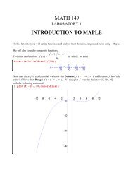
Example: Reproduction of Linear Functions using Gaussian RBFsWe can try to fit the bivariate linear function f (x, y) = (x + y)/2 withGaussians (with ε = 6).fasshauer@iit.edu MATH 590 – Chapter 6 15

Example: Reproduction of Linear Functions using Gaussian RBFsWe can try to fit the bivariate linear function f (x, y) = (x + y)/2 withGaussians (with ε = 6).Figure: Gaussian interpolant to bivariate linear function with N = 1089 (left)and associated abolute error (right).fasshauer@iit.edu MATH 590 – Chapter 6 15

Example: Reproduction of Linear Functions using Gaussian RBFsWe can try to fit the bivariate linear function f (x, y) = (x + y)/2 withGaussians (with ε = 6).Figure: Gaussian interpolant to bivariate linear function with N = 1089 (left)and associated abolute error (right).RemarkClearly the interpolant is not completely planar — not even to machineprecision.fasshauer@iit.edu MATH 590 – Chapter 6 15

Example: Reproduction of Linear Functions using Gaussian RBFsThere is a simple remedy for this problem.fasshauer@iit.edu MATH 590 – Chapter 6 16

Example: Reproduction of Linear Functions using Gaussian RBFsThere is a simple remedy for this problem.Just add the polynomial functionsto the Gaussian basisx ↦→ 1, x ↦→ x, x ↦→ y{e −ε2 ‖·−x 1 ‖ 2 , . . . , e −ε2 ‖·−x N ‖ 2 }.fasshauer@iit.edu MATH 590 – Chapter 6 16

Example: Reproduction of Linear Functions using Gaussian RBFsThere is a simple remedy for this problem.Just add the polynomial functionsto the Gaussian basisProblemx ↦→ 1, x ↦→ x, x ↦→ y{e −ε2 ‖·−x 1 ‖ 2 , . . . , e −ε2 ‖·−x N ‖ 2 }.Now we have N + 3 unknowns, namely the coefficients c k ,k = 1, . . . , N + 3, in the expansionP f (x) =N∑c k e −ε2 ‖x−x k ‖ 2 +c N+1 +c N+2 x +c N+3 y, x = (x, y) ∈ R 2 ,k=1fasshauer@iit.edu MATH 590 – Chapter 6 16

Example: Reproduction of Linear Functions using Gaussian RBFsThere is a simple remedy for this problem.Just add the polynomial functionsto the Gaussian basisProblemx ↦→ 1, x ↦→ x, x ↦→ y{e −ε2 ‖·−x 1 ‖ 2 , . . . , e −ε2 ‖·−x N ‖ 2 }.Now we have N + 3 unknowns, namely the coefficients c k ,k = 1, . . . , N + 3, in the expansionP f (x) =N∑c k e −ε2 ‖x−x k ‖ 2 +c N+1 +c N+2 x +c N+3 y, x = (x, y) ∈ R 2 ,k=1but we have only N conditions to determine them, namely theinterpolation conditionsP f (x j ) = f (x j ) = (x j + y j )/2, j = 1, . . . , N.fasshauer@iit.edu MATH 590 – Chapter 6 16

Example: Reproduction of Linear Functions using Gaussian RBFsWhat can we do to obtain a (non-singular) square system?fasshauer@iit.edu MATH 590 – Chapter 6 17

Example: Reproduction of Linear Functions using Gaussian RBFsWhat can we do to obtain a (non-singular) square system?As we will see below, we can add the following three conditions:N∑c k = 0,k=1N∑c k x k = 0,k=1N∑c k y k = 0.k=1fasshauer@iit.edu MATH 590 – Chapter 6 17

Example: Reproduction of Linear Functions using Gaussian RBFsHow do we have to modify our existing MATLAB program for scattereddata interpolation to incorporate these modifications?fasshauer@iit.edu MATH 590 – Chapter 6 18

Example: Reproduction of Linear Functions using Gaussian RBFsHow do we have to modify our existing MATLAB program for scattereddata interpolation to incorporate these modifications?Earlier we solvedAc = y,with A jk = e −ε2 ‖x j −x k ‖ 2 , j, k = 1, . . . , N, c = [c 1 , . . . , c N ] T , andy = [f (x 1 ), . . . , f (x N )] T .fasshauer@iit.edu MATH 590 – Chapter 6 18

Example: Reproduction of Linear Functions using Gaussian RBFsHow do we have to modify our existing MATLAB program for scattereddata interpolation to incorporate these modifications?Earlier we solvedAc = y,with A jk = e −ε2 ‖x j −x k ‖ 2 , j, k = 1, . . . , N, c = [c 1 , . . . , c N ] T , andy = [f (x 1 ), . . . , f (x N )] T .Now we have to solve the augmented system[ ] [ ] [ A P c yP T=O d 0], (1)where A, c, and y are as before, and P jl = p l (x j ), j = 1, . . . , N,l = 1, . . . , 3, with p 1 (x) = 1, p 2 (x) = x, and p 3 (x) = y. Moreover, 0 isa zero vector of length 3, and O is a zero matrix of size 3 × 3.fasshauer@iit.edu MATH 590 – Chapter 6 18

Example: Reproduction of Linear Functions using Gaussian RBFsProgram (RBFInterpolation2Dlinear.m)1 rbf = @(e,r) exp(-(e*r).^2); ep = 6;2 testfunction = @(x,y) (x+y)/2;3 N = 9; gridtype = ’u’;4 dsites = CreatePoints(N,2,gridtype);5 ctrs = dsites;6 neval = 40; M = neval^2;7 epoints = CreatePoints(M,2,’u’);8 rhs = testfunction(dsites(:,1),dsites(:,2));9 rhs = [rhs; zeros(3,1)];10 DM_data = DistanceMatrix(dsites,ctrs);11 IM = rbf(ep,DM_data);12 PM = [ones(N,1) dsites];13 IM = [IM PM; [PM’ zeros(3,3)]];14 DM_eval = DistanceMatrix(epoints,ctrs);15 EM = rbf(ep,DM_eval);16 PM = [ones(M,1) epoints]; EM = [EM PM];17 Pf = EM * (IM\rhs);18 exact = testfunction(epoints(:,1),epoints(:,2));19 maxerr = norm(Pf-exact,inf)20 rms_err = norm(Pf-exact)/nevalfasshauer@iit.edu MATH 590 – Chapter 6 19

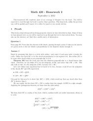
Example: Reproduction of Linear Functions using Gaussian RBFsRemarkExcept for lines 9, 12, 13, and 16 which were added to deal with theaugmented problem RBFInterpolation2Dlinear.m is the sameas RBFInterpolation2D.m.fasshauer@iit.edu MATH 590 – Chapter 6 20

Example: Reproduction of Linear Functions using Gaussian RBFsRemarkExcept for lines 9, 12, 13, and 16 which were added to deal with theaugmented problem RBFInterpolation2Dlinear.m is the sameas RBFInterpolation2D.m.Figure: Interpolant based on linearly augmented Gaussians to bivariate linearfunction with N = 9 (left) and associated abolute error (right).fasshauer@iit.edu MATH 590 – Chapter 6 20

Example: Reproduction of Linear Functions using Gaussian RBFsRemarkExcept for lines 9, 12, 13, and 16 which were added to deal with theaugmented problem RBFInterpolation2Dlinear.m is the sameas RBFInterpolation2D.m.Figure: Interpolant based on linearly augmented Gaussians to bivariate linearfunction with N = 9 (left) and associated abolute error (right).The error is now on the level of machine accuracy.fasshauer@iit.edu MATH 590 – Chapter 6 20

Scattered Data Fitting w/ More General Polynomial PrecisionOutline1 Interpolation with Multivariate Polynomials2 Example: Reproduction of Linear Functions using Gaussian RBFs3 Scattered Data Fitting w/ More General Polynomial Precision4 Almost Negative Definite Matrices and Reproduction of Constantsfasshauer@iit.edu MATH 590 – Chapter 6 21

Scattered Data Fitting w/ More General Polynomial PrecisionMotivated by the example above with linear polynomials we modify theassumption on the form of the solution to the scattered datainterpolation by adding certain polynomials to the expansion, i.e., P f isnow assumed to be of the formP f (x) =N∑c k ϕ(‖x − x k ‖) +k=1M∑d l p l (x), x ∈ R s , (2)where p 1 , . . . , p M form a basis for the M = ( )m−1+sm−1 -dimensional linearspace Π s m−1of polynomials of total degree less than or equal to m − 1in s variables.l=1fasshauer@iit.edu MATH 590 – Chapter 6 22

Scattered Data Fitting w/ More General Polynomial PrecisionMotivated by the example above with linear polynomials we modify theassumption on the form of the solution to the scattered datainterpolation by adding certain polynomials to the expansion, i.e., P f isnow assumed to be of the formP f (x) =N∑c k ϕ(‖x − x k ‖) +k=1M∑d l p l (x), x ∈ R s , (2)where p 1 , . . . , p M form a basis for the M = ( )m−1+sm−1 -dimensional linearspace Π s m−1of polynomials of total degree less than or equal to m − 1in s variables.RemarkWe use polynomials in Π s m−1instead of degree m polynomials sincethis will work better with the conditionally positive definite functionsdiscussed in the next chapter.l=1fasshauer@iit.edu MATH 590 – Chapter 6 22

Scattered Data Fitting w/ More General Polynomial PrecisionSince enforcing the interpolation conditions P f (x j ) = f (x j ),j = 1, . . . , N, leads to a system of N linear equations in the N + Munknowns c k and d l one usually adds the M additional conditionsN∑c k p l (x k ) = 0, l = 1, . . . , M,k=1to ensure a unique solution.fasshauer@iit.edu MATH 590 – Chapter 6 23

Scattered Data Fitting w/ More General Polynomial PrecisionSince enforcing the interpolation conditions P f (x j ) = f (x j ),j = 1, . . . , N, leads to a system of N linear equations in the N + Munknowns c k and d l one usually adds the M additional conditionsN∑c k p l (x k ) = 0, l = 1, . . . , M,k=1to ensure a unique solution.ExampleThe example in the previous section represents the particular cases = m = 2.fasshauer@iit.edu MATH 590 – Chapter 6 23

Scattered Data Fitting w/ More General Polynomial PrecisionRemarkThe use of polynomials is somewhat arbitrary (any other set of Mlinearly independent functions could also be used).fasshauer@iit.edu MATH 590 – Chapter 6 24

Scattered Data Fitting w/ More General Polynomial PrecisionRemarkThe use of polynomials is somewhat arbitrary (any other set of Mlinearly independent functions could also be used).The addition of polynomials of total degree at most m − 1guarantees polynomial precision provided the points in X form an(m − 1)-unisolvent set.fasshauer@iit.edu MATH 590 – Chapter 6 24

Scattered Data Fitting w/ More General Polynomial PrecisionRemarkThe use of polynomials is somewhat arbitrary (any other set of Mlinearly independent functions could also be used).The addition of polynomials of total degree at most m − 1guarantees polynomial precision provided the points in X form an(m − 1)-unisolvent set.If the data come from a polynomial of total degree less than orequal to m − 1, then they are fitted exactly by the augmentedexpansion.fasshauer@iit.edu MATH 590 – Chapter 6 24

Scattered Data Fitting w/ More General Polynomial PrecisionIn general, solving the interpolation problem based on the extendedexpansion (2) now amounts to solving a system of linear equations ofthe form [ A PP T O] [ cd] [ y=0], (3)where the pieces are given by A jk = ϕ(‖x j − x k ‖), j, k = 1, . . . , N,P jl = p l (x j ), j = 1, . . . , N, l = 1, . . . , M, c = [c 1 , . . . , c N ] T ,d = [d 1 , . . . , d M ] T , y = [y 1 , . . . , y N ] T , 0 is a zero vector of length M,and O is an M × M zero matrix.fasshauer@iit.edu MATH 590 – Chapter 6 25

Scattered Data Fitting w/ More General Polynomial PrecisionIn general, solving the interpolation problem based on the extendedexpansion (2) now amounts to solving a system of linear equations ofthe form [ A PP T O] [ cd] [ y=0], (3)where the pieces are given by A jk = ϕ(‖x j − x k ‖), j, k = 1, . . . , N,P jl = p l (x j ), j = 1, . . . , N, l = 1, . . . , M, c = [c 1 , . . . , c N ] T ,d = [d 1 , . . . , d M ] T , y = [y 1 , . . . , y N ] T , 0 is a zero vector of length M,and O is an M × M zero matrix.RemarkWe will study the invertibility of this matrix in two steps.First for the case m = 1,and then for the case of general m.fasshauer@iit.edu MATH 590 – Chapter 6 25

Scattered Data Fitting w/ More General Polynomial PrecisionWe can easily modify the MATLAB program listed above to deal withreproduction of polynomials of other degrees.ExampleIf we want to reproduce constants then we need to replace lines 9, 12,13, and 16 by9 rhs = [rhs; 0];12 PM = ones(N,1);13 IM = [IM PM; [PM’ 0]];16 PM = ones(M,1); EM = [EM PM];fasshauer@iit.edu MATH 590 – Chapter 6 26

Scattered Data Fitting w/ More General Polynomial PrecisionWe can easily modify the MATLAB program listed above to deal withreproduction of polynomials of other degrees.ExampleIf we want to reproduce constants then we need to replace lines 9, 12,13, and 16 by9 rhs = [rhs; 0];12 PM = ones(N,1);13 IM = [IM PM; [PM’ 0]];16 PM = ones(M,1); EM = [EM PM];and for reproduction of bivariate quadratic polynomials we can use9 rhs = [rhs; zeros(6,1)];12a PM = [ones(N,1) dsites dsites(:,1).^2 ...12b dsites(:,2).^2 dsites(:,1).*dsites(:,2)];13 IM = [IM PM; [PM’ zeros(6,6)]];16a PM = [ones(M,1) epoints epoints(:,1).^2 ...16b epoints(:,2).^2 epoints(:,1).*epoints(:,2)];16c EM = [EM PM];fasshauer@iit.edu MATH 590 – Chapter 6 26

Scattered Data Fitting w/ More General Polynomial PrecisionRemarkThese specific examples work only for the case s = 2. Thegeneralization to higher dimensions is obvious but more cumbersome.fasshauer@iit.edu MATH 590 – Chapter 6 27

Almost Negative Definite Matrices and Reproduction of ConstantsOutline1 Interpolation with Multivariate Polynomials2 Example: Reproduction of Linear Functions using Gaussian RBFs3 Scattered Data Fitting w/ More General Polynomial Precision4 Almost Negative Definite Matrices and Reproduction of Constantsfasshauer@iit.edu MATH 590 – Chapter 6 28

Almost Negative Definite Matrices and Reproduction of ConstantsWe now need to investigate whether the augmented system matrix in(3) is non-singular.fasshauer@iit.edu MATH 590 – Chapter 6 29

Almost Negative Definite Matrices and Reproduction of ConstantsWe now need to investigate whether the augmented system matrix in(3) is non-singular.The special case m = 1 (in any space dimension s), i.e., reproductionof constants, is covered by standard results from linear algebra, andwe discuss it first.fasshauer@iit.edu MATH 590 – Chapter 6 29

Almost Negative Definite Matrices and Reproduction of ConstantsDefinitionA real symmetric matrix A is called conditionally positive semi-definiteof order one if its associated quadratic form is non-negative, i.e.,N∑j=1 k=1for all c = [c 1 , . . . , c N ] T ∈ R N that satisfyN∑c j c k A jk ≥ 0 (4)N∑c j = 0.j=1If c ≠ 0 implies strict inequality in (4) then A is called conditionallypositive definite of order one.fasshauer@iit.edu MATH 590 – Chapter 6 30

Almost Negative Definite Matrices and Reproduction of ConstantsRemarkIn the linear algebra literature the definition usually is formulatedusing “≤" in (4), and then A is referred to as conditionally (oralmost) negative definite.fasshauer@iit.edu MATH 590 – Chapter 6 31

Almost Negative Definite Matrices and Reproduction of ConstantsRemarkIn the linear algebra literature the definition usually is formulatedusing “≤" in (4), and then A is referred to as conditionally (oralmost) negative definite.Obviously, conditionally positive definite matrices of order oneexist only for N > 1.fasshauer@iit.edu MATH 590 – Chapter 6 31

Almost Negative Definite Matrices and Reproduction of ConstantsRemarkIn the linear algebra literature the definition usually is formulatedusing “≤" in (4), and then A is referred to as conditionally (oralmost) negative definite.Obviously, conditionally positive definite matrices of order oneexist only for N > 1.We can interpret a matrix A that is conditionally positive definite oforder one as one that is positive definite on the space of vectors csuch thatN∑c j = 0.j=1fasshauer@iit.edu MATH 590 – Chapter 6 31

Almost Negative Definite Matrices and Reproduction of ConstantsRemarkIn the linear algebra literature the definition usually is formulatedusing “≤" in (4), and then A is referred to as conditionally (oralmost) negative definite.Obviously, conditionally positive definite matrices of order oneexist only for N > 1.We can interpret a matrix A that is conditionally positive definite oforder one as one that is positive definite on the space of vectors csuch thatN∑c j = 0.j=1In this sense, A is positive definite on the space of vectors c“perpendicular” to constant functions.fasshauer@iit.edu MATH 590 – Chapter 6 31

Almost Negative Definite Matrices and Reproduction of ConstantsNow we are ready to formulate and proveTheoremLet A be a real symmetric N × N matrix that is conditionally positivedefinite of order one, and let P = [1, . . . , 1] T be an N × 1 matrix(column vector). Then the system of linear equationsis uniquely solvable.[ A PP T 0] [ cd] [ y=0],fasshauer@iit.edu MATH 590 – Chapter 6 32

Almost Negative Definite Matrices and Reproduction of ConstantsProofAssume [c, d] T is a solution of the homogeneous linear system, i.e.,with y = 0.fasshauer@iit.edu MATH 590 – Chapter 6 33

Almost Negative Definite Matrices and Reproduction of ConstantsProofAssume [c, d] T is a solution of the homogeneous linear system, i.e.,with y = 0.We show that [c, d] T = 0 T is the only possible solution.fasshauer@iit.edu MATH 590 – Chapter 6 33

Almost Negative Definite Matrices and Reproduction of ConstantsProofAssume [c, d] T is a solution of the homogeneous linear system, i.e.,with y = 0.We show that [c, d] T = 0 T is the only possible solution.Multiplication of the top block of the (homogeneous) linear system byc T yieldsc T Ac + dc T P = 0.fasshauer@iit.edu MATH 590 – Chapter 6 33

Almost Negative Definite Matrices and Reproduction of ConstantsProofAssume [c, d] T is a solution of the homogeneous linear system, i.e.,with y = 0.We show that [c, d] T = 0 T is the only possible solution.Multiplication of the top block of the (homogeneous) linear system byc T yieldsc T Ac + dc T P = 0.From the bottom block of the system we know P T c = c T P = 0, andthereforec T Ac = 0.fasshauer@iit.edu MATH 590 – Chapter 6 33

Almost Negative Definite Matrices and Reproduction of ConstantsSince the matrix A is conditionally positive definite of order one byassumption the equationc T Ac = 0.implies that c = 0.fasshauer@iit.edu MATH 590 – Chapter 6 34

Almost Negative Definite Matrices and Reproduction of ConstantsSince the matrix A is conditionally positive definite of order one byassumption the equationc T Ac = 0.implies that c = 0.Finally, the top block of the homogeneous linear system states thatAc + dP = 0,so that c = 0 and the fact that P is a vector of ones imply d = 0. □fasshauer@iit.edu MATH 590 – Chapter 6 34

Almost Negative Definite Matrices and Reproduction of ConstantsRemarkSince Gaussians (and any other strictly positive definite radial function)give rise to positive definite matrices, and since positive definitematrices are also conditionally positive definite of order one, thetheorem above establishes the nonsingularity of the (augmented)radial basis function interpolation matrix for constant reproduction.fasshauer@iit.edu MATH 590 – Chapter 6 35

Almost Negative Definite Matrices and Reproduction of ConstantsRemarkSince Gaussians (and any other strictly positive definite radial function)give rise to positive definite matrices, and since positive definitematrices are also conditionally positive definite of order one, thetheorem above establishes the nonsingularity of the (augmented)radial basis function interpolation matrix for constant reproduction.In order to cover radial basis function interpolation with reproduction ofhigher-order polynomials we will introduce (strictly) conditionallypositive definite functions of order m in the next chapter.fasshauer@iit.edu MATH 590 – Chapter 6 35

References IAppendixReferencesBuhmann, M. D. (2003).Radial Basis Functions: Theory and Implementations.Cambridge University Press.Chui, C. K. (1988).Multivariate Splines.CBMS-NSF Reg. Conf. Ser. in Appl. Math. 54 (SIAM).Fasshauer, G. E. (2007).Meshfree Approximation Methods with MATLAB.World Scientific Publishers.Higham, D. J. and Higham, N. J. (2005).MATLAB Guide.SIAM (2nd ed.), Philadelphia.Iske, A. (2004).Multiresolution Methods in Scattered Data Modelling.Lecture Notes in Computational Science and Engineering 37, Springer Verlag(Berlin).fasshauer@iit.edu MATH 590 – Chapter 6 36

References IIAppendixReferencesWendland, H. (2005a).Scattered Data Approximation.Cambridge University Press (Cambridge).Berzolari, L. (1914).Sulla determinazione d’una curva o d’una superficie algebrica e su alcunequestioni di postulazione.Rendiconti del R. Instituto Lombardo, Ser. (2) 47, pp. 556–564.Chung, K. C. and Yao, T. H. (1977).On lattices admitting unique Lagrange interpolations.SIAM J. Numer. Anal. 14, pp. 735–743.Radon, J. (1948).Zur mechanischen Kubatur.Monatshefte der Math. Physik 52/4, pp. 286–300.fasshauer@iit.edu MATH 590 – Chapter 6 37