Quantitative mineral analysis of talc-magnesite ... - Arkisto.gsf.fi

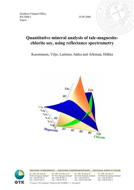
Southern Finland OfficeRS/2006/1 19.09.2006EspooQuantitative mineral analysis of talc-magnesitechloritesoy, using reflectance spectrometryKuosmanen, Viljo, Laitinen, Jukka and Arkimaa, Hilkka

GEOLOGICAL SURVEY OF FINLANDDOCUMENTATION PAGEDate / Rec. no.19.09.2006AuthorsKuosmanen, Viljo, Laitinen, Jukka and Arkimaa,HilkkaType of reportArchive ReportCommissioned byTitle of reportQuantitative mineral analysis of talc-magnesite-chlorite soy, using reflectance spectrometryAbstractQuantitative remote detection of different mineral materials is today an important issue. It can improve identificationof materials and speed up processes. The need for such techniques exists especially in the mining industry andmineral exploration sectors.This work aims to develop the remote sensing method towards quantitative estimation of target minerals in realtime. The target of this case study is drilling soy from the Lahnaslampi talc mine in Sotkamo. The main componentsof this ore are talc, magnesite and chlorite.If we have a soy mixture containing unknown quantities of talc, magnesite and chlorite, can we determine the trueportions of these minerals using only VSWIR reflectance spectral measurement? The answer is yes. This can bedone by means of the principle of physical summation of reflectance. Linear unmixing of the mixed spectra wascarried out first and the physically biased results were corrected using a polynomial correction function. This functionmust be computed separately for mixtures composed of different mineral end-members.In this case study, the mean accuracy of the estimated volumetric portions of talc, magnesite and chlorite from thespectra is 2.6 %. Spectral accuracy is however dependent on the actual background data: volumetric percentages ofmineral powders could be determined at 2-3 % accuracy. The spectral estimation reached this limit, but could not,naturally, exceed the accuracy of the vol-% limit. However, high the signal-to-noise-ratio of the VSWIRreflectancesuggests that the accuracy based on spectral estimation can be higher.The system developed in this work can be used to estimate abundances of three end-members. This method offersa very quick tool for several mineral related applications.KeywordsInfrared, spectroscopy, reflectance, VSWIR, talc, magnesite, chloriteGeographical areaSotkamo, FinlandMap sheet3433Other informationReport serialRSTotal pages18Unit and sectionLanguageEnglishSouthern Finland Office/Land Use and EnvironmentSignature/nameArchive codeRS/2006/1PriceProject code2804004Signature/nameConfidentiality

Contents1 INTRODUCTION 12 SPECTRUM OF A MINERAL MIXTURE 13 TALC, MAGNESITE AND CHLORITE AND THEIR REFLECTANCE 24 TWO-COMPONENT MIXTURES AND THEIR SPECTRA 34.1 2-component powder mixtures 44.2 Linear unmixing of the spectra 55 THREE-COMPONENT MIXTURES AND THEIR SPECTRA 105.1 3-component soy mixtures 105.2 Linear unmixing of spectra of 3-component mixtures 125.3 Solving the mineral quantities by nonlinear correction functions 136 CONCLUSIONS AND DISCUSSION 177 ACKNOWLEDGEMENTS 188 REFERENCES 18FIGURES:Figure 1. Mixed mineral pixel: formation of a sum spectrum of three components eachcovering a 1 , a 2 , and a 3 cm 2 from the surface of the target. The sum spectrum for the observer ina), b) and c) is the same if one or more components are fragmented provided that all parts of thesurface are Lambertian. 2Figure 2. Reflectance spectra of talc, magnesite and chlorite. 3Figure 3. Spectra of talc and chlorite mineral soy mixtures. The respective volume- percentagesof talc and chlorite in the soy mixture are seen in Table 1 columns 1 and 2. 7Figure 4. Original talc fraction versus linearly unmixed talc fraction in talc-chlorite soymixture. 7Figure 5. Spectra of mixtures of talc and magnesite. The respective volume-percentages of talcand magnesite in the soy mixture are seen in Table 1, columns 3 and 4. 8Figure 6 Original talc fraction versus linearly unmixed talc fraction in talc-magnesite soymixture 8Figure 7 Spectra of mixtures of magnesite and chlorite. The respective volume-percentages ofmagnesite and chlorite in the soy mixture are seen in Table 1, columns 5 and 6. 9Figure 8 Original magnesite fraction versus linearly unmixed magnesite fraction in magnesitechloritesoy mixture. 9Figure 9 The actual measured talc, magnesite and chlorite volume percentages from Table 2plotted as fractions (dots) into ternary T-M-C diagram. The red and green numbers indicate talc

and chlorite fractions in triangular coordinates. The black numbers indicate respective x and yvalues in rectangular coordinates. 11Figure 10 The reflectance spectra of 3-component mixtures of talc, magnesite and chlorite. Theend-members were mixed in proportions illustrated in Table 2 and Figure 9. 12Figure 11 The measured talc-magnesite-chlorite fractions and their linearly unmixed biasedestimates from the spectra of the mixed powders. . Camoufage and forward scattering of lightcauses the bias. 13Figure 12 Stereopairs for 'crossed-eye viewing' of the polynomial correction functions whichremove the physically induced optical bias from the unmixing results. 14Figure 13 The unbiased estimated abundances talc, magnesite and chlorite from the spectra. 17TABLES:Table 1. Volume percentages of end-member mineral powders in the respective 2-componentsoy mix-tures. 4Table 2 Percentages of end-member mineral powders in the respective 3-component soy mixtures.10Table 3 Order of polynomial terms 15Table 4 List of the wavelength areas best for unmixing and estimating abundances of talc,magnesite and chlorite and the respective percentual error. 15Table 5 The coefficients k tji for the polynomial terms of z t in Eq 4 for estimating talc content. 16Table 6 The coefficients k mji for the polynomial terms of z m in Eq 5 for estimating magnesitecontent. 16Table 7 The coefficients k cji for the polynomial terms of z c in Eq 6 for estimating chloritecontent. 16

11 INTRODUCTIONQuantitative remote detection of different mineral materials is today an important issue, becauseit can improve identification of materials and speed up processes. The need for such techniquesexists especially in the mining industry and mineral exploration sectors. Mining and other industriesneed estimation of target materials on a more quantitative basis.This case study makes an assessment of mineral powder mixtures of talc, magnesite and chloriteusing VSWIR 1 -spectroradiometric reflectance measurements. These minerals are the main constituentsof several talc ore deposits. The aim is to simulate true drilling soy and to study its mineralcontent. The rock and mineral samples for this study were collected from the Lahnaslampitalc mine in Sotkamo, NE-Finland. The total reflectance spectrum of a multi-component target isformed as a weighted sum of the separate components in that target. The exposed area of eachcomponent within the target determines its weight in that sum.In the case of drilling soy this is a valid relation, but due to surface-active phenomena of minerals,the mineral soys are able to ‘mask’ or camouflage each other in various degrees. Thereforethe quantity of a component mineral in a mixture cannot be estimated by linearly unmixing thespectrum of the mixture, i.e. the ‘mixed pixel’. A non-linear correction term is needed after linearunmixing. This especially concerns those cases where micas and/or clays occur in mixturewith other silicates.The aim of this work is to study the summation of reflectance spectra of talc, magnesite andchlorite (end members) soy in a single measurement, in one pixel. Another aim is to estimate theend member quantities from an unknown mixture of talc, magnesite and chlorite in one pixel.2 SPECTRUM OF A MINERAL MIXTUREThe reflectance spectrum m of a target is a sequence of numbers characterizing the fraction betweenthe reflected electromagnetic radiation [W/ cm 2 ] and the incoming radiation [W/ cm 2 ] as afunction of wavelength. Clark (1999) gives a deeper insight into this topic.Spectral Angle Mapping (SAM) has been a classical and effective mathematical tool for mineralmapping from remote sensing data (Girouard et al 2004, Shippert, P., 1995). Supervised classificationhas been widely used for detecting non-mixed classes. A more exact method is suggestedhere for quantitative estimation of endmembers in a mixed classes case.Let the reflectances of three separate components of a single target, i.e. a Lambertian surface 2 , bem 1 , m 2 and m 3 (vectors) and their coverage areas be a 1 , a 2 , and a 3 cm 2 respectively. The total reflectancer of the entire target surface is:1VSWIR = Visible to Short Wave Infrared electromagnetic radiation, wavelengths from 350 to 2500 nanometres.Spectroradiometry is here used in reflectance mode.2 A Lambertian surface is a surface of perfectly matte properties, which means that it adheres to Lamberts cosinelaw. Lamberts cosine law states that the reflected or transmitted luminous intensity in any direction from an elementof a perfectly diffusing surface varies as the cosine of the angle between that direction and the normal vector of thesurface. As a consequence, the luminance of that surface is the same regardless of the viewing angle. (seehttp://www.schorsch.com/kbase/glossary/lambertian_surface.html )

23r = ∑ αimii=1where αi = ai / (a1+ a2+ a3)The spectrum of a mixture composed of several end-members is - in the ‘simple’ case of surface- formed as a weighted linear combination of the spectra of the components (Figure 1). This relationis valid for any number of end-member components in the mixture.The linear summation of component reflectances is complicated by many factors: In the case ofminerals, the surfaces are not Lambertian and the edges of the fragments are optically differentfrom the 'plain' mineral surfaces. Further, some minerals tend to stick on other minerals and maycamouflage other mineral species in mixtures. However, in the case of volumetric mineral mixtures,the weights α 1 , α 2 , and α 3 are non-linear functions, which can be solved through mathematicalanalysis of the spectra.Figure 1. Mixed mineral pixel: formation of a sum spectrum of three components each covering a 1 , a 2 ,and a 3 cm 2 from the surface of the target. The sum spectrum for the observer in a), b) and c) is the same ifone or more components are fragmented provided that all parts of the surface are Lambertian.The physics of reflection is actually dependent on the surface topography of the object, the particlesize and distribution, the bidirectional scattering characteristics of the surfaces and the incidenceangles of the radiation source (see Hapke 1984 and 1981). In this study, most factors otherthan mineral composition are assumed to be constant and therefore are not dealt with here.3 TALC, MAGNESITE AND CHLORITE AND THEIR REFLECTANCE

3The samples studied in the current work are a set of pure-mineral talc, magnesite and chloriteblocks from the Lahnaslampi mine. Mineralogy of these mineral samples was determined usingX-ray diffractometry and microprobing. The samples were ground with a Retsch mill to a particlesize corresponding to normal drilling soy. The resulting simulated monomineral soys weremixed with each other in various proportions in order to simulate talc ore drilling soy of variouscompositions.Reflectances of the ‘pure’ mineral samples of talc, magnesite and chlorite were measured (Figure3) using the FieldSpecFR-portable spectrometer, which can measure over the VSWIR wavelengthrange, i.e. 350-2500 nanometers. In order to maximize signal-to-noise ratio (S/N ratio),each measurement was repeated 10 times.Figure 2. Reflectance spectra of talc, magnesite and chlorite.4 TWO-COMPONENT MIXTURES AND THEIR SPECTRAThe Spectra of the mineral mixtures were studied from two different points of view: theoreticallinear and experimental mixtures of spectra were studied. The difference between these two revealthe important impact of surface activity on the reflectance spectra of mineral mixtures.

44.1 2-component powder mixturesThe powders of the pure minerals talc and chlorite were mixed in various weight or volume proportions.The mixtures were prepared by adding small portions of chlorite into talc and weighingthe result (Table 1, columns 1 and 2).Table 1. Volume percentages of end-member mineral powders in the respective 2-component soy mixtures.1 2 3 4 5 6TalcV%ChloriteV%TalcV%MagnesiteV%MagnesiteV%ChloriteV%100.0 0.0 100.0 0.0 100.0 0.099.3 0.793.4 6.689.1 10.984.6 15.479.0 21.0 80.0 20.074.7 25.369.1 30.961.6 38.456.5 43.5 60.0 40.0 60.0 40.052.3 47.747.8 52.243.4 56.640.4 59.6 40.0 60.0 40.0 60.036.1 63.933.1 66.928.8 71.223.5 76.519.5 80.5 20.0 80.0 20.0 80.015.9 84.111.9 88.17.5 92.55.7 94.34.2 95.80.0 100.0 0.0 100.0 0.0 100.0Thereafter, the result was transformed into volume percent by weighing 10 cm 3 volumes of thesepowders. Talc, magnesite and chlorite soy weighted 19.5 g, 29.1 g and 18.5 g respectively. Othermixtures were prepared by adding magnesite in a small cup of constant volume into talc or chlorite(Table 1, columns 3-4 and 5-6) and transforming them into volume percentages. The volumetricpercentages contain error, which may range from 0 to 3%, because powder is inhomogeneousand compressible.Reflectances (Figure 3, 5 and 6) of the mixed soys were measured using the FieldSpecFR spectroradiometer.The whole VSWIR wavelength range, i.e. 350-2500 nanometers was covered. Inorder to maximize S/N ratio, each measurement was repeated 10 times.

54.2 Linear unmixing of the spectraLinear spectral unmixing is an important approach to the analysis of hyperspectral data. It considersthat a mixed pixel is a linear combination of p end-members signatures weighted by correspondingabundance fractions.We use here the same mathematical notation as was used by Råde and Westergren (2004) andNielsen (2001, 2002).r = Mα + n , where[ ] Tr = r 1Lr l= l-dimensional mixed spectrum (= mixed pixel)where r j is reflectance over l channels, j varies overwave-lengthi[ m Lm] Tm == l-dimensional signal for end-member i = 1 … pi 1[ 1,K1] Til1 == vector of units, spans albedoM =[ 1, m ,m K ]1 2mp=⎡ m11L⎢⎢MM O⎢⎣1mlLmembers1 mp1Mmpl⎤⎥⎥⎥⎦= (l+1) x p matrix of 1 and end-[ α α L ] Tα = 0, 1α p= coefficients we wish to estimate for fractions(abundances)n == residual, i.e. the variation in r not explained by the[ ] Tn 1Ln llinear model (Eq 2)To solve α from these equations, the sum of squared residuals is n T n (or more generallyT −1n Σ n where Σ n is the dispersion or covariance matrix of the residuals), therefore the partialnT −1derivatives are set to ∂ ( n Σ n) / ∂α= 0 . This will result in the estimatornT −1−1T −1αˆ = (M Σ M) M Σ r with expectation E{ α} ˆ = α andnnT −1−122with dispersion (M ΣnM) . When Σ n= σ I where I is the lxl unit matrix and σ is the varianceof all residuals, V { } = σ (the least squares2case),Eq 1αˆ= (Mn iM)T −1MTrTo evaluate the guality of the model we calculate:2(r~ T ~ T −1TR = r − n Σ n) /~r~r the coefficient of determination ( ~ r = r centered) andns2=( nTΣ−1nn) /( l − p −1)the estimate of residual variance when l-p- 1 > 0

6s = the Root Mean Square ErrorIn the first case of this study, the end-members are the reflectance spectra of talc, magnesite andchlorite illustrated in Figure 2, while the mixed spectra are the two-component mixtures illustratedin Figure 3, 4 and 7. Therefore l = 2151 (number of channels in the spectra) and p = 2(number of end-members in two component mixture).When the talc-chlorite binary mixture spectra (Figure 3) are linearly unmixed (using Eq 1) intofractions of the end-members it can be immediately noticed that the result (Figure 4) underestimatestalc content. This is in line with the result by Mustard and Pieters (1989), who noticed thatthe low albedo minerals tend to be overestimated.The same relation (Figure 6) applies to the unmixing of the talc-magnesite binary mixture spectra(Figure 5). The 'darker' mineral magnesite is overestimated. The magnesite-chorite mixturespectra (Figure 7) behave in the same way (Figure 8). Therefore, these estimates are called biasedestimates. This is a practical example of the fact that chlorite can camouflage talc and magnesite,and that magnesite can camouflage talc. If the unmixing results are mutually compared(Figs 4, 6 and 8) they are not similar, as can be expected.In order to solve the actual volumetric fractions of talc, magnesite and chlorite in pairs from therespective mixture spectra, analytical inversion functions are needed. This task will be solved inthe next chapter on a more general 3-component mixture level.

7Figure 3. Spectra of talc and chlorite mineral soy mixtures. The respective volume- percentages of talcand chlorite in the soy mixture are seen in Table 1 columns 1 and 2.Figure 4. Original talc fraction versus linearly unmixed talc fraction in talc-chlorite soy mixture.

8Figure 5. Spectra of mixtures of talc and magnesite. The respective volume-percentages of talc andmagnesite in the soy mixture are seen in Table 1, columns 3 and 4.Figure 6 Original talc fraction versus linearly unmixed talc fraction in talc-magnesite soy mixture

9Figure 7 Spectra of mixtures of magnesite and chlorite. The respective volume-percentages of magnesiteand chlorite in the soy mixture are seen in Table 1, columns 5 and 6.Figure 8 Original magnesite fraction versus linearly unmixed magnesite fraction in magnesite-chloritesoy mixture.

105 THREE-COMPONENT MIXTURES AND THEIR SPECTRAOur intention is to:• Prepare the 3-component soy mixtures from 'pure' end-member minerals• Measure a reflectance spectrum for each end-member and each 3-component mixture• Carry out linear unmixing of the spectra of each 3-component mixture (mixed pixel).This operation produces the biased estimates for the volumetric fractions of talc, magnesiteand chlorite from the spectra.• Compute nonlinear correction functions, which transform the biased estimates to nonbiasedvolumetric fractions of talc, magnesite and chlorite.• Assess the average residual error of the mathematical estimation of the fractional volumetricproportions for the end-members• Assess the average residual error of the physical estimation as a function of the lower andupper limits of wavelength.5.1 3-component soy mixturesThe three component mixtures of talc, magnesite and chlorite were prepared by adding definitevolumetric quantities (spoons) of each mineral powder into 21 different pots. These quantitiesare transformed into volumetric percentages in Table 2.Table 2 Percentages of end-member mineral powders in the respective 3-component soy mix-tures.TalcV%MagnesiteV%ChloriteV%100.00 0.00 0.0080.00 20.00 0.0060.00 40.00 0.0040.00 60.00 0.0020.00 80.00 0.000.00 100.00 0.0080.00 0.00 20.0060.00 20.00 20.0040.00 40.00 20.0020.00 60.00 20.000.00 80.00 20.0060.00 0.00 40.0040.00 20.00 40.0020.00 40.00 40.000.00 60.00 40.0060.00 0.00 40.0020.00 20.00 60.000.00 40.00 60.0020.00 0.00 80.000.00 20.00 80.000.00 0.00 100.00

11The original volume % are also illustrated by fractions in the ternary talc-magnesite-chlorite (T-M-C) diagram in Figure 9. It is an equilateral triangle in which all sides have the same length 1,if expressed by a fraction or 100, if expressed by percentage. The corners represent 100 % quantityfor talc, magnesite or chlorite. The fraction of each mineral in a mixture is proportional todistance from the opposite side. The average error of volume percentage is 0.0 – 3.0 %.The original fractions z (= V%/100) for talc z t , magnesite z m and chlorite z c are plotted on the x-yplane in the ternary T-M-C diagram (Figure 11) using following formulasEq 2Eq 31x = 1 − z m− z2y =z t32tz t , z m and z c > 0 and z t + z m + z c = 1, when all points are inside the triangleand side of this isosceles triangle = 1.Figure 9 The actual measured talc, magnesite and chlorite volume percentages from Table 2 plotted asfractions (dots) into ternary T-M-C diagram. The red and green numbers indicate talc and chlorite fractionsin triangular coordinates. The black numbers indicate respective x and y values in rectangular coordinates.The mixed powders were measured using the FieldSpecFR portable spectroradiometer overVSIR wavelengths 350-2500 nm. The measurement was repeated 10 times in order to maximisethe S/N ratio. The spectra are illustrated in Figure 10.

125.2 Linear unmixing of spectra of 3-component mixturesSimultaneous linear unmixing of talc, magnesite and chlorite (Figure 2) content was carried outfor the mixed pixels (Figure 10). In unmixing, the number of channels, l, equals 2151 and numberof end-members, p, equals 3 (see the formulas in chapter 4.2). The unmixed fractions are illustratedin Figure 11. Due to the physical camouflage of minerals, the linearly unmixed fractionsexaggerate chlorite and magnesite content. Therefore these quantities are called biased estimates.The bias of the estimates is mainly due to physical properties of the minerals, rather than by instrumentsor computing. Grinding some minerals, particularly micas, tends to produce finegraineddust, which sticks to larger mineral particles. The scattering angle is the angle θ betweenthe forward direction of the incident beam and a straight line connecting the scattering point andthe detector. The scattering of photons by a medium in such a way that most of the photons endup travelling in roughly direction they started, i.e θ < 90 o is called 'forward scattering'. This isalways accompanied by some backscattering (θ > 90 o ). Micaceous dust undoubtedly causes forwardscattering and therefore enhances illumination of dust covered other minerals. This biaswill be removed using nonlinear correction functions.Figure 10 The reflectance spectra of 3-component mixtures of talc, magnesite and chlorite. The endmemberswere mixed in proportions illustrated in Table 2 and Figure 9.

135.3 Solving the mineral quantities by nonlinear correction functionsThe linearly unmixed biased estimates, α 1 for talc, α 2 for magnesite and α 3 for chlorite, wereplotted on x-y plane in the ternary T-M-C diagram (Figure 11) using the formulas of Eq 2 and Eq3.1x = 1 − α2− α123y = α 12α 1 , α 2 and α 3 > 0 and α 1 + α 2 + α 3 = 1 if all points are inside the triangleside of the triangle = 1.Figure 11 The measured talc-magnesite-chlorite fractions and their linearly unmixed biased estimatesfrom the spectra of the mixed powders. . Camoufage and forward scattering of light causes the bias.The optical bias is seen as the movement of the estimate from the original position towards adarker end-member. The bias can be modelled and removed. The shifted x and y values werecorrected using following polynomial functions:2 2t= ∑∑ tji+0 0j iEq 4 z ( x,y)k y x e ( x,y)j iEq 5 z ( x,y)k y x e ( x,y)2m mji+0 02= ∑∑tm

14j iEq 6 z ( x,y)k y x e ( x,y)2c cji+0 02= ∑∑cz t (x,y) is the empirically measured content of talc (volume %) where x and y are the rectangularplane coordinates of the unmixed relative abundances of talc. The polynomial coefficients k tji aredetermined as the residual error e t (x,y) is minimised through least squares fitting. The respectivefunctions with the coefficients k mji , k cji and the residuals e m and e c are calculated for magnesite z mand chlorite z c in the same way.The nonlinear polynomial correction functions are illustrated in Figure 12. An easy way to seethe stereo view is the 'crossed-eye techniques' explained by Starosta 2006. Each stereo view consistsof two images, one for each eye. That means that the first (leftmost) image is for your righteye and the right image is for your left eye. Cross your eyes, so that the pair of images will firstdouble to four, and be somewhat out of focus. Next, slowly uncross your eyes. At some point,the two middlemost images you are seeing will begin to overlap: When you see just three imagesthe overlap is perfect and you will see a complete 3-D image in the middle.Figure 12 Stereopairs for 'crossed-eye viewing' of the polynomial correction functions which remove thephysically induced optical bias from the unmixing results.The physically unbiased estimates, t for talc, m for magnesite and c for chlorite aretm2= ∑∑0220= ∑∑020ktjikymjijxyijxi

15c2= ∑∑020kcjiyjxiThe estimated coefficients for the polynomial terms are given separately for talc, magnesite andchlorite (the coefficients written without t, m and c) in the order shown in Table 3.Table 3 Order of polynomial termsk 00 k 01 x k 02 x 2k 10 y k 11 yx k 12 yx 2k 20 y 2 k 21 y 2 x k 22 y 2 x 2The final mean residual error for talc estimatemean residual error for magnesite estimateE = meantE = meanmetemmean residual error for chlorite estimatetotal mean residual errorE = meancE =e( E + E + E )tm3ccThe final fractional error term E was used to search for an optimal lower and higher boundary forthe wavelength content. This was done through computing E for all lower boundaries between350 nm-2400 nm and higher boundaries between 450 nm – 2500 nm. The wavelength area,which produced the minimal error E = 2.63 %, is surprisingly narrow: 2290 – 2360 nm. However,these wavelengths may represent the most characteristic absorption features for the endmemberminerals (see Figure 2). The ten best wavelength areas are listed in Table 4.Table 4 List of the wavelength areas best for unmixing and estimating abundances of talc, magnesite andchlorite and the respective percentual error.Order ofsignificanceWavelengthlower limitnmWavelengthupper limitnmE %1 2290 2360 2.63092 1390 1620 2.64113 970 1680 2.66104 970 1700 2.67455 1990 2080 2.67676 990 1720 2.67687 2010 2280 2.67708 990 1680 2.67949 1050 1700 2.680410 2290 2480 2.6807Only the best significant wavelengths (2290 – 2360) are listed and used here for estimating thequantities of talc, magnesite and chlorite. Removing the inessential wavelengths naturally decreasesthe time needed for computer interpretation of the data. The coefficients corresponding

16to the polynomial terms in Table 3 are listed in Table 5, 6 and 7 respectively for talc, magnesiteand chlorite.Table 5 The coefficients k tji for the polynomial terms of z t in Eq 4 for estimating talc content.-0.0377 1.2896 0.02960.1046 -0.4671 -2.8539-0.0854 -0.0401 5.4151The average of the absolute values of E t between the true and estimated talc content is 0.0194and the standard deviation of the residual is 0.0292. The correlation coefficient is 0.9955 and therisk value p is < 2.2*10 -16 .Table 6 The coefficients k mji for the polynomial terms of z m in Eq 5 for estimating magnesite content.1.0405 -1.3783 0.2550-0.1224 0.2998 2.9462-0.9058 1.6942 -6.6740The average of the absolute values of E m between the true and estimated magnesite content is0.0315 and the standard deviation of the residual is 0.0420. The correlation coefficient is 0.9904and the risk value p is < 2.2*10 -16 .Table 7 The coefficients k cji for the polynomial terms of z c in Eq 6 for estimating chlorite content.-0.0028 0.0887 -0.28460.0179 0.1673 -0.09230.9912 -1.6541 1.2589The average of the absolute values of E c between the true and estimated chlorite content is0.0279 and the standard deviation of the residual is 0.0427. Correlation coefficient is 0.9898, andthe risk value p is < 2.2*10 -16 .After applying these transformations for removing the physically induced optical bias, the resultingestimated abundances of talc, magnesite and chlorite are as seen in Figure 13.

17Figure 13 The unbiased estimated abundances talc, magnesite and chlorite from the spectra.6 CONCLUSIONS AND DISCUSSIONIf we have a soy mixture containing unknown quantities of talc, magnesite and chlorite, can wedetermine the true portions of these minerals using only VSWIR reflectance spectral measurement?The answer is yes. This can be done by means of the principle of physical summation ofreflectance and unmixing the abundances from the spectrum of a mixture.However, summation of mineral spectra is not generally linear. Minerals normally scatter light(EM-radiation) backwards, but they may scatter forward, too. One mineral species may coverand camouflage another species. Therefore the total reflectance from a multi-component targetdoes not sum up the component reflectances linearly and a nonlinear correction is needed.Linear unmixing of the mixed spectra was carried out first and the results were subsequently correctedusing a polynomial correction function. This function must be calculated separately formixtures composed of different end-members.In this case study, the mean accuracy of the estimated volumetric portions of talc, magnesite andchlorite from the spectra is 2.6 %. Spectral accuracy is however dependent on the actual backgrounddata: volumetric percentages of mineral powders could be determined at 2-3 % accuracy.The spectral estimation reached this limit, but could not, naturally, exceed the accuracy of thevol % limit. However, high S/N ratio of the VSWIR-reflectance suggests that the accuracy basedon spectral estimation can be higher.The system developed in this work can be used to estimate abundances of three end-members.

18This method offers a very quick tool for several applications. When a portable spectrometer isused, the measurement itself lasts 10 seconds and a computed interpretation takes about 1 second.When an imaging spectrometer is used, about 30 000 measurements can be done in 1 secondand they all can be interpreted in a few seconds. This method is recommended for developedfor use in on-line measurements in the mineral industry.7 ACKNOWLEDGEMENTSWe wish to thank Mondo Minerals Oy and especially geologists Ilkka Tuokko and Eero Kuronenfor granting their mineral materials, equipment and other facilities to the authors use.8 REFERENCESClark, R. N., 1999. Chapter 1: Spectroscopy of Rocks and Minerals, and Principles ofSpectroscopy, in Manual of Remote Sensing, Volume 3, Remote Sensing for the EarthSciences, (A.N. Rencz, ed.) John Wiley and Sons, New York, 3 - 58.http://speclab.cr.usgs.gov/PAPERS.refl-mrs/refl4.htmlGirouard, G.,and A.Bannari, A. El Harti and A. Desrochers, 2004. Validated Spectral AngleMapper Algorithm for Geological Mapping: Comparative Study between Quickbird andLandsat-TM. http://www.isprs.org/istanbul2004/comm4/papers/432.pdfHapke, B. 1984. Bidirectional reflectance spectroscopy. 3. Correction for macroscopicroughness. Icarus 59: 41-59.Hapke, Bruce 1981. "Bidirectional Reflectance Spectroscopy: 1. Theory", JGR, 86, 3039-3054.Hapke, Bruce, Eddie Wells 1981. "Bidirectional Reflectance Spectroscopy: 2. Experiments andObservations", JGR, 86, 3055-3060.Starosta, B.: http://www.starosta.com/3dshowcase/ihelp.htmlNielsen, A.A., 2001. Spectral mixture analysis: Linear and semi-parametric full and iteratedpartial unmixing in multi- and hyperspectral imge data. International Journal of ComputerVision 42(1/2), 2001, 17- 37.Nielsen, A. A., 2002. Multiset Canonical Correlations Analysis and Multispectral, Truly MultitemporalRemote Sensing Data. IEEE Transactions on Image Processing 11(3), 293-305.