Guided Construction of a 2D TDDFT code - TDDFT.org

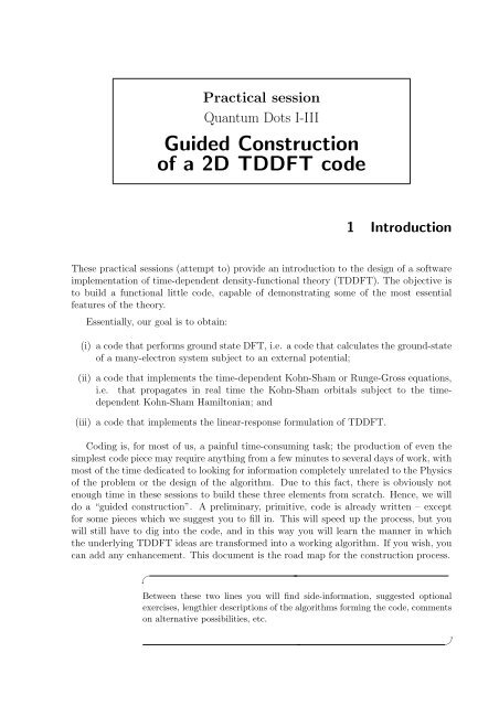
Practical sessionQuantum Dots I-IIIGuided Constructionof a 2D TDDFT code1 IntroductionThese practical sessions (attempt to) provide an introduction to the design of a softwareimplementation of time-dependent density-functional theory (TDDFT). The objective isto build a functional little code, capable of demonstrating some of the most essentialfeatures of the theory.Essentially, our goal is to obtain:(i) a code that performs ground state DFT, i.e. a code that calculates the ground-stateof a many-electron system subject to an external potential;(ii) a code that implements the time-dependent Kohn-Sham or Runge-Gross equations,i.e. that propagates in real time the Kohn-Sham orbitals subject to the timedependentKohn-Sham Hamiltonian; and(iii) a code that implements the linear-response formulation of TDDFT.Coding is, for most of us, a painful time-consuming task; the production of even thesimplest code piece may require anything from a few minutes to several days of work, withmost of the time dedicated to looking for information completely unrelated to the Physicsof the problem or the design of the algorithm. Due to this fact, there is obviously notenough time in these sessions to build these three elements from scratch. Hence, we willdo a “guided construction”. A preliminary, primitive, code is already written – exceptfor some pieces which we suggest you to fill in. This will speed up the process, but youwill still have to dig into the code, and in this way you will learn the manner in whichthe underlying TDDFT ideas are transformed into a working algorithm. If you wish, youcan add any enhancement. This document is the road map for the construction process.✎Between these two lines you will find side-information, suggested optionalexercises, lengthier descriptions of the algorithms forming the code, commentson alternative possibilities, etc.✌

2This is the outline of this handout:• In Section 2, you can find a few words about the two-dimensional electrons gas. Thereason is that, for practical purposes, the code is two-dimensional.• In Section 3, some more theory: the generalised Kohn’s theorem, that will be studiednumerically later.• Section 4 describes how the code is organised in practice.• Finally, the following sections are a step-by-step presentation of the code.2 Two-dimensional problems and quantum dots.The scope of the code is not general: it is a two-dimensional code. The reason to limitthe code in this form is that in this way the computations can be done in very short time(typically seconds or minutes).In principle, however, the extension to the 3D problem is straightforward. The algorithmspresented are essentially the same in the 3D world. In practice, the code that weprovide is specially simple and lacks some of the features that a fully-fledged code has(e.g. non-local pseudopotentials – which are covered elsewhere in this course –, etc). Thisis necessary due to the time limitation. Note, however, that the 2D problem is not only ofacademic interest; the 2D electron gas is subject of very lively and active research, boththeoretically and experimentally.Quantum dots (QDs) are artificial nano-scale devices; essentially they may be viewedas confined electron crowds. Due to their smallness, they exhibit quantum-mechanicalatom-like behaviour (e.g. shell structure). To some extent, we can consider quantum dotsas the basic components of nanoelectronics [1]. Quantum dots are fabricated by confiningmetal or semiconductor conduction-band electrons in a localised region. There are severalways to achieve this localisation; one of them is by making use of semiconductor interfaces.In this case, the movement of the electrons is not possible in the perpendicular directionto the interface and the thickness of the interface region is very small. The resultingstructure is known as the two-dimensional electron gas (2DEG). Laterally, the electronsalso have to be confined applying some kind of potential, which is typically modelled insome simple way.Not surprisingly, DFT has been successfully applied to describe numerous examplesof 2DEG QDs [2]. And, also not surprisingly, TDDFT has also played a role to describeproperties related to excited-states of 2DEG QDs [3]. The program that we will workwith could be a useful tool for this kind of investigations – very active nowadays –, andnot only a classroom exercise.Some important features, however, will not be incorporated: to name a few, we willassume spin-unpolarised calculations, and will not consider the possible presence of a

section 3. Kohn’s theorem, and generalised Kohn’s theorem. 3magnetic field, or the extension to current density-functional theory (CDFT) – ratherrelevant in this field. Regarding numerics, you may find the design of the program, orthe choice of the algorithm, to be sub-optimal, to say the least. We invite you to addany feature, or to improve the code in any manner, as a final exercise or project, if timepermits.✎It is common practice to use the effective mass approximation to describe theelectrons in semiconductors or metals. This number in principle depends onthe kinetic energy of the electron, but if it turns out to be approximatelya constant, the problem is greatly simplified. We may then work with aneffective Hamiltonian:Ĥ =N∑ ˆp 2 N i2mi=1∗ + + ∑i=1ˆv ext (ˆr i ) +N∑ e 2 14πǫ |ˆr i − ˆr j | , (1)For the GaAs semiconductor (very common material in QDs experiments),the effective mass m ∗ is 0.067 times the mass of a free electron.To ease the numerical work, it is convenient to choose the appropriate unitssystem. In atomic, molecular and solid-state Physics, this is usually the socalledatomic units system. If we take the effective mass approximation, it isconvenient to redefine this system of units: We set the effective mass m ∗ = 1,the dielectric constant of the medium ε = 1, Planck’s constant ¯h = 1 and theabsolute charge of the electron e = 1. In the CGS-unit system, we then getthe effective mass atomic units.The unit of length is then then effective bohr a ∗ 0 = (ε/m∗ )a 0 (a 0 is the Bohrradius); the unit of energy is the effective Hartree Ha ∗ = (m ∗ /ε 2 )Ha, and theunit of time is the effective atomic time, u ∗ t = (m e /¯h)a ∗ 0 . It is assumed in thecode that this effective system of units is used. (In a typical GaAs lattice,ε = 12.4ε 0 ).In the following, we will assume this system of units (and will the omit thesymbols with asterisks, unless necessary).i

4✎It is easy to prove the generalised Kohn’s theorem. Assuming a two-dimensionalproblem, such as the one we are interested in, we depart from a Hamiltonianin the form:Ĥ =N∑i=1ˆp 2 i,x2m + N ∑i=1ˆp 2 i,y2m + N ∑i=112 mω2 0(ˆx 2 i + ŷ 2 i ) +N∑û(ˆr i − ˆr j ), (2)i

4.1. Compilation 5> tar -xzvf qd-0.1.0.tar.gzThis should produce a directory qd-0.1.0. If you navigate into it, you will find a bunchof files and directories; the two important directories are src and doc. In the latter youwill find a pdf with this document (along with the man and info pages of the code, whichare rather empty). The important files – the source files that you will have to modify, arein src.4.1 CompilationThe first task is to compile and install the code. This should be rather straightforward inthe machines of the school: First of all, decide where you want to install the code; sinceyou do not have root privileges in that machine, you can for example install softwarelocally in your home directory, in a subdirectory called, e.g. software:> mkdir $HOME/softwareThen you do the usual configure-make-make install sequence:> ./configure --prefix=$HOME/software> make> make installAfter this, your $HOME/software should contain at least three directories: bin, infoand man. The former contains the code, qd. The info directory contains the qd.infofile, in principle an on-line code manual; and man/man.1 contains a man page for qd.✎If you don’t have some background with UNIX-like machines, probably youare not familiar with info or man documentation. You do not need them forthese sessions. In any case, you can consult the info file by typing:> info -f $HOME/software/share/info/qd.infoThe man/man1 directory contains the manual page of the code. You get it bytyping:[7]> man -l $HOME/software/share/man/man1/qd.1In fact, both manuals are rather empty. We have included them here since boththe info and the man formats are two of the most standard documentationschemes in software development, and it can be useful for you to learn how

6to use and manage them. The sources to generate these documents are theqd.texinfo file (the info file is generated from this source with the makeinfoprogram), and the qd.pod file (the man file is generated from this source withthe pod2man program).Being qd the code name, you just have to type:✌> $HOME/software/bin/qdqd 0.1.0Written by The 2006 Benasque TDDFT School.Copyright (C) 2006 The 2006 Benasque TDDFT SchoolThis program is free software; you may redistribute it under the terms ofthe GNU General Public License. This program has absolutely no warranty.to run the code. If you add $HOME/software/bin to your PATH environment variable,you will have no need of specifying the full path, and you can just type qd. Note that byrunning qd without any command line argument, it merely emits a greeting message, asillustrated above.Whenever you make a modification to the code, you have to recompile it by typingmake, and re-install it by typing make install.Hopefully, the installation process should run smoothly in the machines installed inBenasque. However, we have on purpose constructed a code following, at least partially,the “standard” coding conventions of the free software community: gnu autotools,possibility of info documentation, etc. By making use of the autotools, in particular, weensure that the porting of the code to other machines / operating systems / compilersshould pose no problems. We thought that constructing the code in this manner is a wayto demonstrate these techniques to those of you who are unfamiliar with them.4.2 Running modesThe code is written in a combination of C and Fortran – in fact, most of the code isFortran, and this is the part that you will have to work on. The program has, in fact, amain function written in C: the main that you can see in the file qd.c. However, the onlypurpose of this program is parsing the command line options, and calling the appropriateFortran procedure afterwards. The Fortran code is linked as a library (libqdf.a) to thismain function [8].The program qd accepts command line arguments; you can learn which by typing qd--help:

section 5. The mesh. 7> qd --helpUsage: qd [OPTION...]qd is a simple, pedagogical implementation of TDDFT for 2D systems.-c, --coefficients Generates coefficients for the discretization-e, --test_exponential Tests the exponential-g, --gs Performs a ground state calculation-h, --test_hartree Tests the Poisson solver-l, --test_laplacian Tests the Laplacian-s, --strength_function Calculates the strength function-t, --td Performs a time-dependent calculation-x, --excitations Performs a LR-TDDFT calculation-?, --help Give this help list--usage Give a short usage message-V, --version Print program versionReport bugs to .The options determine in which running mode the code will operate. This mode ispassed by the C main to the Fortran subroutine fortranmain, written in the file qdf.f90.Depending on the mode, fortranmain will in turn call different routines. These routines,and their dependencies, are contained in the rest of the Fortran files *.f90.The files have “holes”, that we suggest you to fill in. Also, note that the code ispurposely simple-minded to increase clarity; you may think of ideas to improve on thealgorithms for performance (or just elegance) reasons. The “holes” are marked by thedelimiters:!!!!!! MISSING CODE X...!!!!!! END OF MISSING CODEThe number X is an identifier number. Possible solutions for the missing parts are offeredin file missing.f90. You may choose to code those tasks that you find more useful foryour purposes, or else copy directly from missing.f90, and improve the code with ideasof your own, or with other suggestions.5 The mesh.The first choice to make when building an electronic-structure code is that of the basis set.Numerous possibilities are available [9]. For this code we will choose the most intuitive ofthem all: a real space mesh. In other words, the functions (wave functions, densities, etc)are represented by the values that they take on a selected set of points in real space [10].

8A given function f, is represented by its set of values {f i } on those points. We mayunderstand these values as the components of a vector of an N-dimensional Hilbert space(N being the number of points of our mesh).In the Fortran 90 module mesh, in file mesh.f90, you can find the definition of thepoints that conform the mesh, and the procedures that manage the functions defined inthis mesh. The comments explain the purpose of the module, and of each procedure. Ifthey are not that clear (which will usually happen), you will have to read the code tounderstand what is its purpose.The key procedures in the mesh module are the functions that calculate the dot products,and the functions that calculate the Laplacian of a function. And here you willsee the first piece of missing code; one first coding task that you may attempt is theconstruction of the Laplacian operator.We need the coefficients {c k } +Nk=−N∂ 2 f∂x 2(x 0) = c 0 f(x 0 ) +to build up an expression in the form:N∑−N∑c k f(x k ) + c k f(x k ). (4)k=1k=−1This expression provides an approximation for the second derivative of a function f ata mesh point x 0 , in terms of the values of f at the neighbour points (and itself) x k =kh,k = −N,...,N. You may then build the Laplacian simply by doing ∇ 2 = ∂2 f∂x + ∂2 f2 ∂y . 2In order to get these coefficients, you will need to run the code in “coefficients” mode,by passing the -c or the --coefficients command line argument. The program isalready prepared for a 9-point formula (N = 4) of the second derivative.Visit the coeff.f90 file. It contains the source for the run-mode that generates thecoefficients necessary to build a real-space discretisation of the second order derivative (orany other derivative).> qd -cqd 0.1.0Written by The 2006 Benasque TDDFT School.Copyright (C) 2006 The 2006 Benasque TDDFT SchoolThis program is free software; you may redistribute it under the terms ofthe GNU General Public License. This program has absolutely no warranty.c(0) = -0.2847222E+01c( 1: n) = 0.1600000E+01 -0.2000000E+00 0.2539683E-01 -0.1785714E-02c(-1:-n) =0.1600000E+01 -0.2000000E+00 0.2539683E-01 -0.1785714E-02✎

section 5. The mesh. 9For the curious, it is maybe worthed a little explanation on what we have justdone.The most common approach to the electronic structure problem (either withDFT or with any other method) is the expansion of the wave functions (andrelated functions) in terms of a set of basis functions. This approach hastwo important properties, which may be easily derived from the variationalprinciple: (i) The approximate ground-state energy obtained with a given basisset is always an upper bound to the exact value; any supplement to the basis setwill yield a lower energy; (ii) The energy displays a quadratic convergence withincreasing basis set size. Despite these two nice features, basis set expansionis not the only approach to the electronic structure problem. An alternativeare the “real-space” methods, which rely on the representation of functionsdirectly on a real-space grid, either regular (as the one we are using) or adaptedto the problem at hand.In a real-space implementation, the functions are represented in a real spacegrid, i.e., we know their values on a selected set of sampling points, {x j } M j=1 ,which typically are arranged in a regular mesh (in the following, we will assumea one-dimensional problem; the extension to two or three dimensional problemswill be done later):f ≡ {f(x j )} j=1,...,M . (5)We want to calculate its n-th derivative in a finite difference scheme.Let us call x 0 = 0, and let us assume that we want to get the n-th derivative off in x 0 = 0, f (n) (x = 0). As input information, we will use the values of f atN points to the right, and N points to the left, besides f(x 0 ): {f(x k )} N k=−N .The objective is to obtain a linear expression of the form:f (n) (x 0 ) = c 0 f(x 0 ) +N∑−N∑c k f(x k ) +k=1k=−1c k f(x k ). (6)The problem is then to obtain the set of coefficients c k . For that purpose, weconsider the set of polynomials:Their n-th derivatives are:⎧⎪⎨g (n)l(x) =⎪⎩g l (x) = x l , l = 0, . . .,2N . (7)l(l − 1)...(l − n + 1)x l−n , n < ln! , n = l0 , n > lIn x = x 0 = 0:g (n)l(x 0 ) = δ nl n! . (9)We may then join Eq. 6 and 9 to obtain 2N + 1 equations. To clarify ideas,let us begin by approximating the first derivative, n = 1:l = 0 : g (1)0 (x 0) : 0 = c 0 + ∑ Nk=1 c k + ∑ −Nk=−1c kl = 1 : g (1)1 (x 0) : 1 = 0 + ∑ Nk=1 c k x k + ∑ −Nk=−1c k x kl = 2 : g (1)2 (x 0) : 0 = 0 + ∑ Nk=1 c k x 2 k + ∑ −Nk=−1c k x 2 k. . . : . . . : . . . = . . .l = 2N : g (1)2N (x 0) : 0 = 0 + ∑ Nk=1 c k x 2Nk + ∑ −Nk=−1c k x 2Nk(8)(10)

10It is useful to setup this linear system in matrix form. We define:x T = [x 1 , . . .,x N , x −1 , . . .,x −N ] , (11)c T = [c 1 , . . .,c N , c −1 , . . .,c −N ] , (12)⎡⎤x 1 . . . x N x −1 . . . x −NxA(x) =2 1 . . . x 2 ⎢N x 2 −1 . . . x 2 −N⎥⎣ . . . . . . . . . . . . . . . . . . ⎦ , (13)x 2N1 . . . x 2NN x 2N−1 . . . x 2N−Nand the n-th unit vector in the 2N dimensional space:e T n = [0, . . .,,0, n 1, 0, . . .,0] . (14)The coefficient c 0 will always be c 0 = − ∑ Nk=1 c k − ∑ −Nk=−1c k . The rest of thecoefficients may be derived from the resulting system, which, for n = 1, is:A(x)c = e 1 (15)It is very easy to generalise this expression for higher derivatives: the n-thderivative coefficients may be obtained through:A(x)c = n!e n (16)Note that, up to now, we have not enforced a regular mesh; the positions {x k },measured with respect to the “problem” point x 0 = 0, are arbitrary. It is clearfrom the previous formulas, how to build finite differences schemes with irregularmeshes: for each point in the mesh, one has to solve the previous linearsystem built with its neighbouring points, and obtain the resulting coefficients(which will be different for each point). In laplacian subroutine, however,we have assumed a regular mesh. The neighbouring points of a given pointx 0 = 0 in a regular mesh can be easily described by:x k = kh, k = −N, . . .,N . (17)We may now illustrate the procedure with the simplest example: approximationto the first derivative with N = 1, i.e. only two neighbouring points. Thematrix equation is:⎡⎢⎣⎤1 1 1⎥0 h −h ⎦0 h 2 (−h) 2⎡⎢⎣⎤c 0⎥c 1c −1⎦ =⎡⎢⎣010⎤⎥⎦ . (18)Solving this linear system one obtains the well known formula: [12]f ′ (x 0 ) = f(x 1) − f(x −1 )2h. (19)The programcoeff is setup to provide the N = 4 approximation to the secondderivative. However, subroutine coeff is more general and can be used to getarbitrary derivatives, out of an arbitrary number of points, distributed nonuniformlyaround the problem point.As an exercise, you may try to implement derivatives of various orders, andcheck how the errors behave with increasing approximation orders.✌

section 6. Visualisation 11Before proceeding, it is important to test that the Laplacian is actually working; youmay test the Laplacian that you have built by running in the test-laplacian mode(-l or --test-laplacian). Take a look at the test laplacian.f90 file. It defines aGaussian distribution in the form:n(r) = 12πα e−r2 /α 2 , (20)(which, incidentally, is normalised: ∫ d 3 r n(r) = 1). The program calculates numericallythe Laplacian of this function, and compares it to the exact result which may be easilyobtained analytically. You may see how the accuracy depends on the ratio between the“hardness” parameter α and the grid spacing, and on the order of discretisation.✎Some work suggestions:• An interesting exercise is to check how the discretisation order (the numberof points you take in the finite difference formula) affects the errorin the calculation of the Laplacian. The key concept is to figure outhow the dependency of the error with the grid spacing changes with thediscretisation order.• The procedure in the file coeff.f90 does not only contain the codenecessary to obtain a second derivative, but derivatives of any order. Itcould be useful to use this feature and build, in module mesh, a routinethat calculates the gradient of a function.• Both in coeff.f90 and in mesh.f90, the discretisation order is hardwired.It would be interesting to allow for more flexibility by, e.g., introducinga new command line argument that reads in this number.The grid spacing, as you will see, is hard wired in module mesh. Also, the size of thereal-space box in which the systems are to be contained, is hard wired. However, notethat you can change these numbers in any moment if required.✌6 VisualisationIn some places of the code (and anywhere you want to put them), there are some callsto the output subroutine, in the output.f90 file. These calls print out to some file thefunctions in the 2D grid. They may be easily plotted with the gnuplot command splot.For the previous example, you will get e.g. the rho file with the Gaussian function, whoseplot is depicted in Fig. 1.

12"rho"0.080.070.060.050.040.030.020.010-25 -20 -15 -10-505101520252015105025 -25-20-15-10-5Figure 1: Gaussian function, as depicted by gnuplot.Of course, you may use any other visualisation program of your choice, and change theoutput function to suit your needs. For example, it may be interesting to see functionsonly along one given axis (normal “xy” plots), instead of 3D plots such as the one youobtain with the “splot” command of gnuplot.7 Setting up the Hamiltonian7.1 Number of states, number of electronsTake a look at the module states in file states.f90: It holds the number of occupiedand unoccupied orbitals that are to be considered. In our simple example, we will alwaysconsider spin-unpolarised calculations with doubly occupied KS orbitals. The modulealso contains the variables that contain the wave functions. Any procedure that needs toaccess the number of states or electrons, or the wave functions, should get access to thismodule through an use states statement.7.2 The external potentialNow you must define the external potential that confines the quantum dot. For thatpurpose, you must visit the external pot subroutine in the epot.f90 file. You may play

7.3. The Hartree potential 13with different potentials; for our first example we will need a harmonic potential in theform:V har (r) = 1 2 ω2 0r 2 . (21)For example, to use numbers of the order of the ones in the calculations presented inRef. [11] (maybe it is worthed to read that paper to get an idea of what we will be doinglater), set ω to 0.22 Ha ∗ . In a following example, we will make use of a quartic potential:A reasonable value for α in this case is 0.00008.V quar (r) = αr 4 . (22)7.3 The Hartree potentialThe following task is providing the code with a procedure to calculate the Hartree potentialout of a given density:∫V H [n](r) = d 3 r n(r′ )|r − r ′ | . (23)It turns out that this old problem continues to be one of the key computational challenges.In one and two-dimensional problems, one may actually use the obvious and slow solution:performing directly the sum on the grid. If {r i } denote the set of grid points:V H [n](r i ) = ∑ jn(r j )δv . (24)|r i − r j |In this equation, δv denotes the volume (surface, in 2D) surrounding each grid point(δv = ∆ 2 if ∆ is the grid spacing in 2D). In case of using an interaction in the form ofthe Yukawa potential, the equation must change accordingly:V H [n](r i ) = ∑ je −γ|r i−r j | n(r j )δv . (25)|r i − r j |✎Of course, you encounter an infinity problem when i = j. The way to circumventthis problem in 2D is:V H [n](r i ) = ∑ j≠in(r j )|r i − r j | δv + 2∆√ πn(r i ). (26)which is the algorithm that you may implement. We also invite you the workof thinking why the previous equation appropriately approximates the Hartreepotential.

14The infinity problem also appears in the Yukawa case. You may also want toprove that in this case, the i = j term should be 2πn(r i ) 1 − e−γ∆/√ π, whichγreduces to the Coulomb case when γ → 0.✌Unfortunately, this easy scheme is slow, and becomes unpractical when the size of thesystem grows – it is easy to see that it is an O(N 2 ), algorithm, where N is number ofmesh points. In 3D one should not try to use it.An alternative is to perform the integral in Fourier space; by making use of the convolutiontheorem, it is easy to see that in the plane wave representation, the Coulomb(or Yukawa) interaction is diagonal. In the case of the Yukawa interaction (the Coulombcase is easily obtained by taking γ → 0):ũ H (G) =2πγ √ ,1 + G2γ 2Ṽ H [n](G) = ũ H (G)ñ(G). (27)However, when applying this technique to the Coulomb interaction (and also to theYukawa interaction, depending on the magnitude of γ) for finite or aperiodic systems,one encounters one difficulty inherently linked to the plane wave representation: a planewave representation necessarily implies periodic boundary conditions, and replication ofthe original charge density in an infinite array. Since the Coulomb interaction is longranged,the simple application of the previous equations (27) includes the interactions ofthe replicas with the original system. This must be avoided. One possible solution is todefine a cutoff on the interaction, e.g.:{ 1u R , r < RH(r) =r(28)0 , r > ROne then uses ũ R H(G) in Eqs. (27).✎Due to the lack of time, we have purposely shortened the discussion of theHartree problem in the main text. Numerous authors have addressed theproblem; our vanity leads us to cite our own work on the subject [26], whichdescribes the plane wave solution, although in the 3D case (other referencesmaybe found therein).In the 2D case, and considering – as we have, in this program – a distributionof charge n placed in a square of side L, the procedures begins by placingit in a bigger square of side (1 + √ 2)L, padding with zeros the extra space.Then one defines an interaction in the form of Eq, (28), with R = √ 2L.It is easy to see that this guarantees that the interaction does not changewithin the original charge distribution, but at the same time avoids interactionbetween neighbouring cells. Then one needs to get the Fourier transform ofthe interaction, ũ R H (G) (prove this!):∞∑ũ R H(G) = R J k (RG)/(RG), (29)k=1

7.4. The exchange and correlation terms 15where J k is the Bessel function of order k.In the Yukawa case, however, one needs not to define a cutoff, since the potentialis short-ranged by definition. The solution is to define the bigger celllarge enough to make the interaction between cells negligible, and then applyEqs. (27) directly.Both options, for the Coulomb and for the Yukawa case, are implemented inthe poisson module.✌To practice some programming, you may want to code the simple solution of Eq. (26),in subroutine poisson sum in the poisson module (file poisson.f90). In this module,you may see that one needs to set through the values of some variables, which interactionto use (Coulomb or Yukawa), what is the value of the Yukawa parameter in case of usingit, and which method to use (the direct sum, or the plane waves approach).To try out the accuracy of the implemented schemes, you may want to take a look atthe program test hartree and run it. First, you should read the source code of the testitself, to try to understand how it is built and what it does.✎The implementation of Eq. 29 is an excellent numerical exercise, by the way.First, it is interesting to understand where this equation comes from, for whichyou will need to understand a little bit of the theory that we have just mentioned.Then, one must supply a numerical procedure that calculates the righthand side of Eq. 29; you will find, in module poisson, two possible solutions(functions besselint, one of them is commented out). We suggest you to tryto understand how they work, and compare their relative efficiencies. Then,you may try to improve them – if this is the case please let us know how!✌7.4 The exchange and correlation termsNow it is time to define the exchange and correlation term, which are placed in filevxc.f90. The subroutine that you have to use is vxc lda, which provides the exchangeand correlation potential and energies in the local density approximation (LDA). Theexpressions are:∫E x [n] =∫E c [n] =d 3 r n(r)ε HEGx (n(r)); v x [n](r) = δE x[n]δn(r) . (30)d 3 r n(r)ε HEGc (n(r)); v c [n](r) = δE c[n]δn(r) . (31)ε HEGx (n) and ε HEGc (n) are the exchange and correlation energy per particle, respectively,of the 2D HEG of density n.

16✎The exchange term may be derived analytically (obvious exercise: derive it):x (n) = − 4√ 23 √ √ n. (32)πε HEGThe correlation term, however, is much more involved. One has to resort tonumerical results (typically of Quantum Monte-Carlo type), which are laterparameterised for easy use in DFT codes. We have chosen the expression parameterisedby Attaccalite and coworkers [27], which for the spin-unpolarisedcase, has the form:ε HEGc (n) = a + (br s + crs 2 + drs) 3 × Ln(1 +er s + fr 3/2s1+ gr 2 s + hr 3 swhere r s is the Wigner-Seitz radius of the 2D HEG (r s = 1/ √ πn).), (33)You may find the generalised subroutines for the spin-polarised case in theoctopus distributions. But we suggest you to write your own version, at leastfor the exchange case:(i) You may easily derive the exchange term for a homogeneous electron gas ofarbitrary polarisation ξ = n ↑ − n ↓n ↑ + n ↓by making use of the identity (spin-scalingidentity):E x [n ↑ , n ↓ ] = 1 2 E x[2n ↑ ] + 1 2 E x[2n ↓ ] . (34)[][The result is ε HEGx (n, ξ) = 1 2(1 + ξ) 3/2 + (1 − ξ) 3/2 ) ε HEGx (n, 0).](ii) Generalise the given subroutines to allow for spin polarised cases.✌7.5 The interactionSubroutine interaction pot in file ipot.f90 has the task of building the terms of theKohn-Sham potential that arise from the electronic interaction: the Hartree and exchangeand correlation terms. It is useful if one writes it in such a way that it is easy to disconnectany of the terms at will, as it is done in the suggested solution in file missing.f90.Alternatively, you can introduce the distinction by allowing the interaction to be anew command-line argument, so that you do not need to recompile the code when youwant to change.Finally, in file hpsi.f90, you have to fill two subroutines: hpsi and zhpsi. Theyshould apply the Kohn-Sham Hamiltonian on an input wavefuction, respectively real orcomplex.

section 8. The SCF cycle, and the ground state program. 178 The SCF cycle, and the ground state program.• It is now time to build one of the mains procedures: the gs subroutine, in chargeof obtaining the ground state Kohn-Sham orbitals. Note that this subroutine, inthe gs.f90 file, consists essentially of some initialisations, and a call to the scfsubroutine, explained below and which performs the self-consistent cycle.• An essential step in each step of the self-consistent procedure is the diagonalisationof the current approximation to the Kohn-Sham Hamiltonian (the exact one atthe end of the cycle). For this task we have implemented a conjugate-gradientsalgorithm in conjugate gradients subroutine in cg.f90 file. We have chosen toimplement the simple yet successful scheme suggested by H. Jiang, Baranger andYang [13].✎The computational research on eigensolvers starts with the works of Jacobi,long time before the existence of computers. Until the 1960s, thestate of the art is dominated by the QR algorithm and related schemes,suitable for the full diagonalisation of general, albeit small, matrices.The eigenproblem has thereafter proved to be ubiquitous in all disciplinesof Science; In Ref. [14] you may find introductions to the topic.In our case, we are confronted with the algebraic eigenproblem thatemerges from the real-space discretisation of the Kohn-Sham equations(a similar problem arises when other representations, e.g., plane waves,are used). The Kohn-Sham operator is the sum of a potential term (typicallynon-local, although not severely non-local) and a partial differentialoperator. In most DFT electronic-structure method, the solution tothis eigenproblem is the most time-consuming part of the calculations.Some key features of this problem are:– Large size. Typically, the matrix dimension is 10 5 -10 6 (smaller, inthe 2D case). Not even modern supercomputers may store the fullmatrix in memory; one requires solvers that need only to know howto operate the Hamiltonian on a vector.– Sparsity. This is the reason that facilitates the solution, despitethe enormous dimensions. The non-null elements of the matrix arenormally a few rows around the diagonal – its number dependingon the order of discretisation of the Laplacian operator. Non-localpseudopotentials add more non-diagonal terms.– Hermiticiy. The Hamiltonian of a physical system should be anobservable.– One is interested only on the smallest eigenvales, i.e. one only needsone small part of the spectrum, not the 10 5 -10 6 eigenpairs.– Usually, approximations to the eigenpairs are available. The reasonis that the eigenproblem has to be solved at each iteration in theSCF cycle. One can use the solutions obtained in the previous stepas initial guesses for the present step.

18– Typically, and related to the previous point, the solution algorithmsare iterative, i.e. the solutions are obtained by iterative improvementof approximate guesses.This is a shallow enumeration of typical approaches:– The implemented eigensolver is a conjugate gradients method, verymuch in the spirit of the approaches described in the papers citedin Ref. [15]. However, the preconditioning employed in these references,which is based on the fact that the kinetic term is diagonalin a plane wave approach, cannot be used in our real space case.– Another option is the preconditioned block-Lanczos algorithm [19]implemented by Saad and collaborators, already used for DFT electroniccalculations. In this case, the preconditioning is based ofhigh-frequency filtering in real space.– Another Lanczos-type eigensolver, namely the one implemented inthe arpack package [16]. [20]– And yet another free implementation of the blocked-Lanczos eigensolveris the trlan package. [21] Regarding this approach, and theLanczos approach to the eigenproblem, see Refs. [14, 22, 23].– Finally, another (related) and commonly invoked algorithm suitablefor this type of calculation is the Davidson algorithm [17],and, more recently, the Jacobi-Davidson scheme [18]. The preciseimplementation that we have tried is the JDQR package [24].• The scf subroutine, in the scf file, takes care of closing the self-consistent cyclethat solves the Kohn-Sham equations. The basic algorithm is depicted in Fig. 2;you may practice some programming by implementing it in some way in the scfsubroutine.✎Figure 2 suggests that the input density (the density that defines theKohn-Sham Hamiltonian at each SCF cycle step ĤKS[n (i) ]) is the outputdensity of the previous step (the density obtained from the wavefunctions that results of the diagonalisation of the Hamiltonian of theprevious step). This doesn’t work properly, and one has to mix thisoutput density with the densities of previous iterations to guarantee theconvergence. The simplest method is the linear mixing:n (i+1) = αn (i)output + (1 − α)n(i) , (35)for some mixing parameter α. You may implement this simple (yet verysafe) scheme; more sophisticated and much more efficients options aregiven in Ref. [25].• Now the gs program should be finished. Run it at will to test it and check thateverything works fine.✌✌

section 8. The SCF cycle, and the ground state program. 19n 0 (r)v KS [n](r)ĥ KS [n]ψ i = ε i ψ in(r) = ∑ i |ψ i (r)| 2noconverged?yesendFigure 2: Flow-chart depicting a generic Kohn-Sham calculationIf you use the confining potential defined in Eq. (21) and only one occupied orbital(i.e. one quantum dot with only two orbitals) you should get some output similarto:SCF CYCLE ITER # 69diff = 1.0075E-071 7.60044118E-01 8.57155697E-06SCF CYCLE ENDEDdiff = 8.0597E-08Etot = 8.5714E-011 7.60044201E-01 8.57493997E-06✎You may check how the eigenvalues depend on the strength of the interaction.This you can do by varying the Yukawa constant, or in a different manner bypre-multiplying the Coulomb interaction with a “coupling constant”:û(ˆr i − ˆr j ) = λ r , (r = |ˆr i − ˆr j |). (36)Note that this coupling constant λ must also affect the exchange and correlationterms in a not-so-obvious way. It will also be interesting to see, depending

20on the shape of the confining potential, how the many-body excitation energiesdiffer from the differences in eigenvalues.• The total energy. One of the numbers that you get is the total energy of theelectrons, which, if you have studied some DFT, you will know that it is:E[n 0 ] = T S [n 0 ] + U[n 0 ] + E ext [n 0 ] + E xc [n 0 ], (37)where n 0 is the ground-state density of the system, T S [n 0 ] is the kinetic energy ofa system of non-interacting electrons with density n 0 (i.e. the Kohn-Sham system),U[n 0 ] is the Hartree energy, E ext [n 0 ] is the energy originated from the externalpotential, and E xc [n 0 ] is the exchange and correlation potential.The previous expression may be rewritten as:N∑∫E[n 0 ] = ε i − U[n 0 ] + E xc [n 0 ] − d 3 rv xc (⃗r)n 0 (⃗r). (38)i=1We suggest you to prove the identity, both theoretically and numerically. In fileenergy.f90 an implementation of this last expression. But it would be interestingto have code for both expressions; in this way we have an extra check of the goodbehaviour of the code.✌9 Propagators, and the time-dependent program.• First, take a look at the main subroutine of the time-dependent mode: td. In thiscase, you just need to read the file td.f90, since in fact all that this subroutine doesis calling at the end the propagate subroutine.• There is nothing exciting in subroutine propagate.f90, as you will see. The keyparameters that define the propagation (total time of simulation, and time step) aredefined in the prop time and dt variables. Note that at each time step one needs torecalculate the Hamiltonian – TDDFT is a problem that involves time-dependentHamiltonians, no matter if there is an external perturbation or not.The real work of propagating the wave functions is done by the propagator subroutine.• The subroutine that implements the approximator to the quantum mechanical propagatorÛ(t + ∆t,t) is written in thepropagator subroutine in thenpropagator.f90file. You will be told about propagators in other parts of the School; in this subroutinewe have implemented the following approximation (you are welcome to tryout other possibilities):Û(t + δt) ≈ exp{−i δt2 ĤKS(t + δt)} exp{−i δt2 ĤKS(t)}, (39)

section 10. Checking the GKT. 21where the (in principle unknown) ĤKS(t + δt) is approximated by considering thedensity that results of the wavefunctions obtained by the crude estimation:φ i = exp{−iδtĤKS(t)}φ i (t). (40)• The previous algorithm requires the computation of the action of the exponentialof the Hamiltonian. For this purpose, it calls the exponential subroutine, which isthe main object of the expo module in the exponential.f90 file.Elsewhere we will comment on numerical algorithms suited for this particular andimportant task. The most obvious you can imagine: truncating the Taylor expansionof the exponential to a certain order:k∑ (−iδt) kexp{−iδtĤKS}φ = Ĥ ki=0k!KSφ . (41)This one you have to supply. Then you will see that there are other two options,which in fact implement the same algorithm, the so-called Lanczos-based approximationto the exponential. One of them is a simple-minded implementation of thealgorithm, whereas the other makes use of the expokit package, a free library thatimplements the same idea in a more elaborate way. For the purpose of running thecode, you may want to try them all and finding out which one of them is faster foreach particular problem.10 Checking the GKT.We now have working ground-state and time-dependent codes. We can thus make ourfirst TDDFT calculations.• We will start with a two-electron quantum dot, modelled by a harmonic potential,such as the one defined in Eq. (21). Once that you have obtained its ground-state,you may start the program in td mode to get its evolution. For that purpose,however, you have to setup a few things:– In propagate subroutine, variables prop time and dt. Regarding the former,one needs to do a simulation long enough to “see” the frequencies that one isseeking. For the purpose of our tests, a propagation of about 2000 effectivemassatomic units should be enough (notice that we are doing calculations verysimilar to the ones presented in Ref. [11], where these values are also taken).– In perturbation subroutine, the shape and magnitude of the initial perturbation.For the purpose of obtaining the optical absorption cross section, onetypically uses a perturbation in the form:φ i (r,t = 0) = e ik·r φ GSi (r). (42)One may setup the magnitude of the perturbation k and its direction.

22Then, one can run the program in td mode. The program sends to standard outputthe total energy of the system at each time step; since the many-body Hamiltonianis time independent, this magnitude should be conserved. If it is not, you mustrethink the time-step, or the characteristics of the propagation algorithm. Also, thefile dipole is written as the program evolves. It contains three columns: the time,the dipole in direction x, and the dipole in direction y. This is the signal from whichone may obtain the excitation energies.Then you may analyse where the excitations lie by taking the sine Fourier transformof the dipole signal. For that purpose, we have put a very simple run mode, -s or--strength function, whose source is in the sf.f90 file. You may learn how itworks by reading its comments.Take a look then at the spectrum. The key questions are: how many spectral peaksdo we get? At what energies?• Now repeat the exercise, but changing to a Yukawa form for the inter-electronicinteraction (setting interaction to YUKAWA in the poisson module. You also haveto specify the γ parameter (gamma variable). A value of 2.0 a.u. −1 is reasonable.Notice that now you have to disconnect (or change, if you feel like doing that work)the exchange and correlation parts of the potential.✎Yes, we cannot use the usual expressions for the exchange and correlation potential.The reason is that they are deduced assuming a Coulomb interaction.For the exchange-term, if you are curious, one can derive the exchange energyper particle of a homogeneous fermion gas interacting through Yukawa’spotential. The result is (for 2D):ε x (n) = − γ 2 { 2F 1 (− 1 2 , 1 −8πn; 2;2 γ 2 ) − 1} , (43)where 2 F 1 (a, b; c; x) is the so-called Gauss hypergeometric function.(i) Derive the previous equation. (Hint: – at least this is what I did – Followthe derivation of the Coulomb exchange energy per particle for a HEG, forexample, in Ref. [28], considering 2D instead of 3D, and Yukawa interactioninstead of Coulomb interaction). [Please let me know if you obtain a differentresult, since I did not check previous equation with any other source...](ii) Does the previous equation reduce to the Coulomb expression for γ = 0?(iii) Implement the previous equation in the code, in order to get a localdensity approximation for the exchange of a Yukawa-electrons gas. (Hint:The hypergeometric functions are defined in the GSL library. We already haveinterfaces to GSL functions in the file gslwrappers.c, so you just have toadd the appropriate one.).I have not even tried to think about the correlation term..• The question is now: how does the new spectrum compare with the one in whichthe Coulomb interaction is used?✌

section 11. Linear-Response TDDFT 23• Now, if you still feel like working, repeat previous tests, but using the quartic potentialof Eq. (22) – or any other external potential that you find more suitable.You should see that (i) there is no longer one single peak in the response (note thatthere may be large differences in the strengths of the different peaks) and (ii) theresponse obtained when using different forms for the inter-electronic interaction isno longer the same.11 Linear-Response TDDFTFinally, we have arranged an almost-complete code that performs TDDFT calculationswithin the linear response formalism [29]. This is not the place to derive the equationsthat are actually solved; let us just present them very quickly. Let us assume that wehave obtained the set of occupied states {φ i } (in the following, i and k run over occupiedstates) and a set of unoccupied states {φ j } (in the following j and l run over unoccupiedstates). You may obtain these states with the gs program, by setting at will the N occand N empty variables.In the linear response formalism, the excitation energies may be obtained by solvingthe following eigenvalue equations (the excitation energies are the square roots of theeigenvalues):QF I = Ω 2 IF i . (44)The matrix Q is m-dimensional, where m is the number of occupied-unoccupied KS orbitalpairs. It is defined to be:√Q ij,kl = δ ik δ jl ωkl 2 + 2√λ ij ω ij K ij,kl λ kl ω kl . (45)In this equation, ω ij = ε j −ε i , the difference of the corresponding eigenvalues. λ ij = f i −f jis the difference in occupation numbers of the orbitals. The key magnitude is the couplingmatrix K:1K ij,kl = 2〈φ i φ j ||r − r ′ | |φ kφ l 〉 + 2〈φ i φ j | δv xc[n](r ′ )|φ k φ l 〉 . (46)δn(r)Very importantly, in the LDA, the second term may be simplified:δv xc [n](r ′ )δn(r)= δ(r − r ′ ) dv xc[n(r)]. (47)dnFrom now on, we leave you on your own, since this handout is getting too large. Yourtask is now to read the excitations program in excitations.f90 file, and see how theprevious equations are implemented, adding whatever pieces may be missing. Then youcan run any of the models of quantum-dots that you wish, and see how these resultscompare with the previous approaches.

24 REFERENCES, COMMENTS, ETC.✎Typically, the previous calculations of the excitation energies is complementedwith the calculation of their strengths. By reading any of the classical referencesof linear response within TDDFT [29], you may locate the appropriateexpressions and implement them (all the necessary quantities are already calculatedpreviously).✌References, Comments, etc.[1] See, for example, R. C. Ashori, Nature 379, 413 (1996); M. A. Kastner, Phys. Today46, 24 (1993); P. L. McEuen, Science 278, 1729 (1997).[2] Some (rather random) examples: E. Räsanen et al, Phys. Rev. B 67, 235307 (2003);H. Jiang, H. Baranger and W. Yang, Phys. Rev. Lett. 90, 026806 (2003); M. Koskinen,M. Manninen and S. M. Reinmann, Phys. Rev. Lett. 79, 1389 (1997); M. Pi etal, Phys. Rev. B 57, 14783 (1998).[3] More (also random) examples: Ll. Serra et al, Phys. Rev. B 59, 15290 (1999); E.Lipparini et al, Phys. Rev. B 60, 8734 (1999).[4] W. Kohn, Phys. Rev. 15, 1242 (1961).[5] L. Brey, N. F. Johnson and B. I. Halperin, Phys. Rev. B 40, 10647 (1989).[6] Some examples: L. Bertini and M. Mella, Phys. Rev. A 69, 042504 (2004); J. M.Ugalde, C. Sarasola and X. López, Phys. Rev. A 56, 1642 (1997).[7] Alternatively, you may setup the MANPATH environment variable to contain$HOME/software/man, so that you then only need to type man qd.[8] Of course, you may not agree with the choice of languages. We use Fortran, biased byour own experience – experience shared, in fact by the larger part of the electronicstructure community. We have chosen to illustrate how the deficiencies of Fortranmay be cured by mixing in the same program different languages – in this case,C permits to include in a standard way, command line arguments (not allowed inFortran 90).[9] Some well known options:• “Traditional” localised basis sets (e.g. Gaussians, Slater type orbitals); for aclassical reference of this approach, see A. Szabo and N. S. Ostlund, ModernQuantum Chemistry, (Dover Publications, Mineola, New York, 1996).• Plane waves; J. Ihm, A. Zunger and M. L. Cohen, J. Phys. C: Solid State Phys.12, 4409 (1979); J. Ihm, Rep. Prog. Phys. 51, 105 (1988).

REFERENCES, COMMENTS, ETC. 25• Finite elements; S. R. White, J. W. Wilkins and M. P. Teter, Phys. Rev. B 39,5819 (1989).• Wavelets; K. Cho, T. A. Arias, J. D. Joannopoulos and P. K. Lam, Phys. Rev.Lett. 71, 1808 (1993).• Wannier functions; N. Marzari and D. Vanderbilt, Phys. Rev. B 56, 12847(1997).• Cubic splines; E. Hernández and M. J. Gillan and C. M. Goringe, Phys. Rev. B55, 13485 (1997).• etc.[10] Arguably, the real-space mesh representation is not a basis set. For a discussion,see, e.g.: C.-K. Skylaris, O. Diéguez, P. D. Haynes and M. C. Payne, Phys. Rev. B66, 073103 (2002); P. Maragakis, J. Soler and E. Kaxiras, Phys. Rev. A 64, 193101(2001).[11] A. Puente and Ll. Serra, Phys. Rev. Lett. 83, 3266 (1999).[12] Fornberg and Sloan [12] provided an algorithm to obtain the coefficients withoutsolving the linear system: B. Fornberg and D. M. Sloan, in Acta Numerica 1994,edited by A. Iserles (Cambridge University Press, 1994), pp. 203-267.[13] H. Jiang, H. U. Baranger and W. Yang, Phys. Rev. B 68, 165337 (2003).[14] Y. Saad, Numerical methods for large eigenvalue problems, Manchester UniversityPress (Manchester, 1992); Z. Bai, J. Demmel, J. Dongarra, A. Ruhe and H. van derVorst (Eds.), SIAM (Philadelphia, 2000).[15] M. P. Teter, M. C. Payne and D. C. Allan, Phys. Rev. B 40, 12255 (1989); M. C.Payne, M. P. Teter, D. C. Allan, T. A. Arias and J. D. Joannopoulos, Rev. Mod.Phys. 64 1045 (1992).[16] D. S. Sorensen, SIAM J. Matrix Anal. Appl. 13, 357, 1992.[17] E. R. Davidson, J. Comput. Phys. 17, 87 (1975)[18] G. L. G. Sleijpen and H. A. van der Vorst, SIAM Review 42, 267 (2000).[19] Y. Saad, A. Stathopoulos, J. Chelikowsky, K. Wu and S. Öğüt, BIT 36, 1 (1996).[20] arpack can be found at http://www.caam.rice.edu/software/ARPACK/.[21] trlan can be found at http://www.nersc.gov/~kswu/.[22] A. Stathopoulos, Y. Saad and K. Wu, Technical report of the Minnesota SupercomputerInstitute, University of Minnesota, UMSI 96/123 (1996).[23] K. Wu and H. Simon, Technical report of the Lawrence Berkeley National Laboratory,41412 (1998).

26 REFERENCES, COMMENTS, ETC.[24] D. R. Fokkema, G. L. G. Sleijpen and H. A. van der Vorst, SIAM J. Sci. Comput.20, 94 (1998).[25] D. D. Johnson, Phys. Rev. B 38, 12807 (1988); D. R. Bowler and M. J. Gillan, Chem.Phys. Lett. 325, 473 (2000).[26] A. Castro, M. J. Stott and A. Rubio, Can. J. Phys. 81, 1151 (2003).[27] C. Attaccalite, S. Moroni, P. Gori-Giorgi and G. B. Bachelet, Phys. Rev. Lett. 88,256601 (2002).[28] J. P. Perdew and S. Kurth, in: C. Fiolhais, F. Nogueira and M. A. L. Marques (Eds.)A Primer in Density Functional Theory, Lectures Notes in Physics 620, (SpringerVerlag, Berlin, 2003), Ch. 1.[29] E. K. U. Gross, J. F. Dobson, M. Petersilka, in: R. F. Nalewajski (Ed.) Density FunctionalTheory (Springer-Verlag, Berlin, 1996), p.81; M. Petersilka, U. J. Gossmannand E. K. U. Gross, Phys. Rev. Lett. 76, 1212 (1996); M. E. Casida, in: D. P. Chong(Ed.) Recent Advances in Density-Functional Methods, Part I (World Scientific, Singapore,1995), p. 155; M. E. Casida, in: J. M. Seminario (Ed.) Recent Developmentsand Applications of Modern Density Functional Theory (Elsevier, Amsterdan, 1996),p. 391; C. Jamorski, M. E. Casida and D. R. Salahub, J. Chem. Phys. 104, 5134(1996); G. Onida. L. Reining and A. Rubio, Rev. Mod. Phys. 74, 601 (2002).