Introduction to the octopus code - TDDFT.org
Introduction to the octopus code - TDDFT.org
Introduction to the octopus code - TDDFT.org

You also want an ePaper? Increase the reach of your titles
YUMPU automatically turns print PDFs into web optimized ePapers that Google loves.
Practical session<br />
oc<strong>to</strong>pus I-II<br />
<strong>Introduction</strong> <strong>to</strong> <strong>the</strong> oc<strong>to</strong>pus<br />
<strong>code</strong><br />
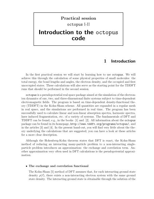
1 <strong>Introduction</strong><br />
In <strong>the</strong> first practical session we will start by learning how <strong>to</strong> use oc<strong>to</strong>pus. We will<br />
achieve this through <strong>the</strong> calculation of some physical properties of small molecules: <strong>the</strong><br />
<strong>to</strong>tal energy, <strong>the</strong> bond lengths and angles, <strong>the</strong> electron density, and <strong>the</strong> occupied and first<br />
unoccupied states. These calculations will also serve as <strong>the</strong> starting point for <strong>the</strong> <strong>TDDFT</strong><br />
runs that should be performed in <strong>the</strong> second session.<br />
oc<strong>to</strong>pus is a pseudopotential real space package aimed at <strong>the</strong> simulation of <strong>the</strong> electronion<br />
dynamics of one, two, and three-dimensional finite systems subject <strong>to</strong> time-dependent<br />
electromagnetic fields. The program is based on time-dependent density-functional <strong>the</strong>ory<br />
(<strong>TDDFT</strong>) in <strong>the</strong> Kohn-Sham scheme. All quantities are expanded in a regular mesh<br />
in real space, and <strong>the</strong> simulations are performed in real time. The program has been<br />
successfully used <strong>to</strong> calculate linear and non-linear absorption spectra, harmonic spectra,<br />
laser induced fragmentation, etc. of a variety of systems. The fundamentals of DFT and<br />
<strong>TDDFT</strong> can be found, e.g., in <strong>the</strong> books [1] and [2]. All information about <strong>the</strong> oc<strong>to</strong>pus<br />
package can be found in its homepage, http://www.tddft.<strong>org</strong>/programs/oc<strong>to</strong>pus/, and<br />
in <strong>the</strong> articles [3] and [4]. In <strong>the</strong> present hand-out, you will find very little about <strong>the</strong> <strong>the</strong>ory<br />
underlying <strong>the</strong> calculations that are suggested; you can have a look at <strong>the</strong>se articles<br />
for a more clear description.<br />
Although <strong>the</strong> Hohenberg-Kohn <strong>the</strong>orem states that DFT is exact, <strong>the</strong> Kohn-Sham<br />
method of reducing an interacting many-particle problem <strong>to</strong> a non-interacting singleparticle<br />
problem introduces an approximation: <strong>the</strong> exchange and correlation term. Ano<strong>the</strong>r<br />
approximation very often used in DFT calculations is <strong>the</strong> pseudopotential approximation.<br />
• The exchange and correlation functional<br />
The Kohn-Sham [5] method of DFT assumes that, for each interacting ground state<br />
density ρ(⃗r), <strong>the</strong>re exists a non-interacting electron system with <strong>the</strong> same ground<br />
state density. The interacting ground state is obtainable through <strong>the</strong> solution of <strong>the</strong>
2<br />
Kohn-Sham equations<br />
[<br />
− 1 ∫<br />
2 ∇2 + v ext (⃗r) +<br />
]<br />
ρ(⃗r)<br />
|⃗r − ⃗r ′ | d ⃗r ′ + v xc ([ρ];⃗r) ϕ i (⃗r) = ǫ i ϕ i (⃗r) , (1)<br />
with <strong>the</strong> electronic density given by<br />
ρ(⃗r) =<br />
N∑<br />
|ϕ i (⃗r)| 2 , (2)<br />
i=1<br />
and <strong>the</strong> <strong>to</strong>tal energy of <strong>the</strong> system is<br />
∫<br />
E KS [ρ(⃗r)] = T s [ρ(⃗r)] + ρ(⃗r)v ext (⃗r)d⃗r + 1 2<br />
∫ ρ(⃗r1 )ρ(⃗r 2 )<br />
|⃗r 1 − ⃗r 2 | d⃗r 1d⃗r 2 + E xc [ρ(⃗r)] . (3)<br />
ϕ i (⃗r) are <strong>the</strong> Kohn-Sham wave functions, T s [ρ(⃗r)] is <strong>the</strong> non-interacting kinetic<br />
energy, v ext is <strong>the</strong> external potential and E xc [ρ(⃗r)] and v xc ([ρ];⃗r) are, respectively,<br />
<strong>the</strong> exchange and correlation energy and potential. E xc is an unknown object and<br />
includes all <strong>the</strong> non-trivial many-body effects required <strong>to</strong> make KS <strong>the</strong>ory exact.<br />
Several approximations <strong>to</strong> E xc have been proposed. The most used is <strong>the</strong> local density<br />
approximation (LDA). In this approximation E xc [ρ(⃗r)] is taken <strong>to</strong> be <strong>the</strong> exchange<br />
and correlation energy of a homogeneous electron gas with density ρ = ρ(⃗r).<br />
Although <strong>the</strong>re exists an exact expression for <strong>the</strong> exchange energy in this model, <strong>the</strong><br />
exact value of <strong>the</strong> correlation energy is known only in <strong>the</strong> limit of very high densities.<br />
Ceperley and Alder [6] did a Monte Carlo simulation of <strong>the</strong> homogeneous electron<br />
gas at several densities. Several parameterizations of <strong>the</strong> correlation energy for any<br />
density [7, 8] were <strong>the</strong>n obtained interpolating <strong>the</strong> Monte Carlo results. One particularly<br />
simple parameterization was proposed by Perdew and Zunger [7], and this<br />
option may be used by oc<strong>to</strong>pus. You can, of course, choose o<strong>the</strong>r xc functionals...<br />
• Exchange and correlation functionals in <strong>TDDFT</strong><br />
The time-dependent Kohn-Sham equations are<br />
i ∂ ]<br />
∂t ϕ i(⃗r, t) =<br />
[− ∇2<br />
2 + v KS(⃗r, t) ϕ i (⃗r, t) . (4)<br />
Here <strong>the</strong> time-dependent Kohn-Sham potential is <strong>the</strong> sum of <strong>the</strong> external timedependent<br />
potential, v ext (⃗r, t), a Hartree term v H (⃗r, t), and <strong>the</strong> exchange-correlation<br />
potential:<br />
∫ ρ(⃗r, t)<br />
v KS (⃗r, t) = v ext (⃗r, t) +<br />
|⃗r − ⃗r ′ | d ⃗r ′ + v xc ([ρ];⃗r, t) . (5)<br />
As in <strong>the</strong> time-independent case, <strong>the</strong> density of <strong>the</strong> interacting system can be obtained<br />
from <strong>the</strong> time-dependent Kohn-Sham orbitals<br />
∑occ<br />
ρ(⃗r, t) = |ϕ i (⃗r, t)| 2 . (6)<br />
i
section 1. <strong>Introduction</strong> 3<br />
The time-dependence of <strong>the</strong> exchange and correlation potential introduces <strong>the</strong> need<br />
for an approximation beyond <strong>the</strong> one made in <strong>the</strong> time-independent case. The simplest<br />
method of obtaining a time-dependent xc potential consists in assuming that<br />
<strong>the</strong> potential is <strong>the</strong> time-independent xc potential evaluated at <strong>the</strong> time-dependent<br />
density, i.e.,<br />
v xc ([ρ];⃗r, t) ≃ v xc ([ρ];⃗r)| ρ≡ρ(⃗r,t)<br />
. (7)<br />
This is called <strong>the</strong> adiabatic approximation. If <strong>the</strong> time-independent xc potential chosen<br />
is <strong>the</strong> LDA, <strong>the</strong>n we obtain <strong>the</strong> so-called adiabatic local density approximation<br />
(ALDA). This approximation gives remarkably good excitation energies but suffers<br />
from <strong>the</strong> same problems as <strong>the</strong> LDA, most notably <strong>the</strong> exponential fall-off of <strong>the</strong><br />
xc potential. If a strong laser pushes <strong>the</strong> electrons <strong>to</strong> regions far from <strong>the</strong> nucleus,<br />
ALDA should not be expected <strong>to</strong> give an accurate description of <strong>the</strong> system.<br />
O<strong>the</strong>r options for <strong>the</strong> time-dependent xc potential are, e.g., <strong>the</strong> orbital-dependent<br />
potentials like <strong>the</strong> exact exchange functional (EXX) (usually in <strong>the</strong> Krieger-Li-<br />
Iafrate (KLI) approximation).<br />
• Pseudopotentials<br />
The many-electron Schrödinger equation can be greatly simplified if electrons are<br />
divided in two groups: valence electrons and inner core electrons. The electrons<br />
in <strong>the</strong> inner shells are strongly bound and do not play a significant role in <strong>the</strong><br />
chemical binding of a<strong>to</strong>ms, thus forming with <strong>the</strong> nucleus an inert core. Binding<br />
properties are almost completely due <strong>to</strong> <strong>the</strong> valence electrons, specially in metals<br />
and semiconduc<strong>to</strong>rs. This separation implies that inner electrons can be ignored,<br />
reducing <strong>the</strong> a<strong>to</strong>m <strong>to</strong> an inert ionic core that interacts with <strong>the</strong> valence electrons.<br />
This suggests <strong>the</strong> use of an effective interaction, a pseudopotential, that gives an<br />
approximation <strong>to</strong> <strong>the</strong> potential felt by <strong>the</strong> valence electrons due <strong>to</strong> <strong>the</strong> nucleus and<br />
<strong>the</strong> core electrons. This can significantly reduce <strong>the</strong> number of electrons that have<br />
<strong>to</strong> be dealt with. Moreover, <strong>the</strong> pseudo wave functions of <strong>the</strong>se valence electrons<br />
are much smoo<strong>the</strong>r in <strong>the</strong> core region than <strong>the</strong> true valence wave functions, thus<br />
reducing <strong>the</strong> computational burden of <strong>the</strong> calculations.<br />
Modern pseudopotentials are obtained by inverting <strong>the</strong> free a<strong>to</strong>m Schrödinger equation<br />
for a given reference electronic configuration, and forcing <strong>the</strong> pseudo wave<br />
functions <strong>to</strong> coincide with <strong>the</strong> true valence wave functions beyond a certain cu<strong>to</strong>ff<br />
distance. The pseudo wave functions are also forced <strong>to</strong> have <strong>the</strong> same norm as <strong>the</strong><br />
true valence wave functions, and <strong>the</strong> energy pseudo eigenvalues are matched <strong>to</strong> <strong>the</strong><br />
true valence eigenvalues. Different methods of obtaining a pseudo eigenfunction<br />
that satisfies all <strong>the</strong>se requirements lead <strong>to</strong> different non-local, angular momentum<br />
dependent pseudopotentials. Some widely used pseudopotentials are <strong>the</strong> Troullier<br />
and Martins [9] potentials, <strong>the</strong> Hamann [10] potentials, <strong>the</strong> Vanderbilt [11] potentials<br />
and <strong>the</strong> Hartwigsen-Goedecker-Hutter [12] potentials. The default potentials<br />
used by oc<strong>to</strong>pus are of <strong>the</strong> Troullier and Martins type, although you can also opt<br />
for <strong>the</strong> HGH potentials.<br />
Besides <strong>the</strong>se usual DFT approximations, <strong>the</strong> use of oc<strong>to</strong>pus implies ano<strong>the</strong>r approximation,<br />
which stems from <strong>the</strong> particular calculation method used.
4<br />
• The choice of <strong>the</strong> mesh<br />
In oc<strong>to</strong>pus <strong>the</strong> Kohn-Sham equations are discretized on a finite mesh in real space.<br />
This means that derivatives are evaluated using a finite differences method (oc<strong>to</strong>pus<br />
uses by default a 9-point rule for <strong>the</strong> laplacian, although o<strong>the</strong>r rules can be chosen)<br />
and integrals are weighted sums over <strong>the</strong> grid points. The mesh is by default uniform,<br />
but <strong>the</strong> <strong>code</strong> allows for curvilinear meshes that adapt better <strong>to</strong> <strong>the</strong> problem<br />
geometry. The grid points play <strong>the</strong> role of <strong>the</strong> ‘basis functions’ of <strong>the</strong> methods<br />
where an expansion of <strong>the</strong> Kohn-Sham wave functions in some bases is employed<br />
(e.g., plane-waves or Gaussian wave functions). But, contrary <strong>to</strong>, e.g., plane-waves,<br />
this ‘basis set’ is not variational. Care must be taken <strong>to</strong> ensure that <strong>the</strong> calculations<br />
are converged with respect <strong>to</strong> <strong>the</strong>se basis fuctions. This implies performing calculations<br />
with different grid spacings. As <strong>the</strong> combination of pseudopotentials and <strong>the</strong><br />
LDA will always introduce a ∼0.1 eV error, <strong>the</strong> convergence with grid spacing is<br />
good enough when energy differences vary by less than 0.1 eV.<br />
2 First session<br />
Objectives<br />
Tasks<br />
• Get a working knowledge of <strong>the</strong> oc<strong>to</strong>pus input file;<br />
• Calculate <strong>the</strong> ground state for some small molecules (Na 2 , C 2 H 2 , and SiH 4 ) using<br />
different exchange and correlation functionals (LDA, GGA, and EXX);<br />
• Study <strong>the</strong> convergence of <strong>the</strong> calculations;<br />
• Plot <strong>the</strong> density, potential, and wave functions;<br />
• Calculate some unoccupied states;<br />
• Start a linear response calculation.<br />
1. Convergence of <strong>the</strong> <strong>to</strong>tal energy with respect <strong>to</strong> <strong>the</strong> grid spacing<br />
Move <strong>to</strong> <strong>the</strong> direc<strong>to</strong>ry ∼/molecules/. There you will find three input files (c2h2.inp,<br />
na2.inp, and sih4.inp), for three different systems. Pick <strong>the</strong> file corresponding <strong>to</strong><br />
<strong>the</strong> system assigned <strong>to</strong> you and take a look at <strong>the</strong> input variables.<br />
✎<br />
Information on <strong>the</strong> input variables is available on <strong>the</strong> file:<br />
/usr/local/doc/oc<strong>to</strong>pus.pdf<br />
or else at <strong>the</strong> <strong>code</strong> online manual:
section 2. First session 5<br />
http://www.tddft.<strong>org</strong>/programs/oc<strong>to</strong>pus/wiki/index.php/Manual.<br />
You will notice that <strong>the</strong> input file is ra<strong>the</strong>r short. This means that all <strong>the</strong> missing<br />
input variables will be given some reasonable default values. In particular, you will<br />
not find in <strong>the</strong> input files any information nei<strong>the</strong>r on <strong>the</strong> exchange and correlation<br />
functional <strong>to</strong> be used nor on <strong>the</strong> pseudopotentials. If you were assigned an exchange<br />
and correlation functional different from <strong>the</strong> default Perdew-Zunger LDA you will<br />
have <strong>to</strong> add some variables <strong>to</strong> <strong>the</strong> input file. Find out which variables <strong>to</strong> add and<br />
type <strong>the</strong>m in. Fill in <strong>the</strong> following table.<br />
✌<br />
Molecule being studied:<br />
Geometry<br />
Box type<br />
Box size<br />
Grid spacing<br />
XC functional<br />
Pseudopotentials<br />
Do a test run of oc<strong>to</strong>pus by copying xxx.inp <strong>to</strong> inp and typing, e.g.:<br />
prompt$ oc<strong>to</strong>pus > xxx.out<br />
xxx represents <strong>the</strong> system you will be studying. The <strong>code</strong> prints out some information<br />
<strong>to</strong> standard output, and that is why it is good <strong>to</strong> redirect standard output <strong>to</strong><br />
some file like xxx.out. If you want <strong>to</strong> see <strong>the</strong> output as it progresses, you can do:<br />
prompt$ oc<strong>to</strong>pus | tee xxx.out<br />
The run should take a few minutes. This way it is not necessary <strong>to</strong> put it in <strong>the</strong><br />
background. For long runs, it is better <strong>to</strong> hide it, so that a terminal crash will not<br />
s<strong>to</strong>p <strong>the</strong> run:<br />
prompt$ oc<strong>to</strong>pus > xxx.out 2>&1 &<br />
At <strong>the</strong> end of <strong>the</strong> run you will see three new direc<strong>to</strong>ries: tmp, status and static.<br />
The first two hold information that is normally only useful for <strong>the</strong> internal work<br />
of <strong>the</strong> <strong>code</strong>, and in general you do not have <strong>to</strong> worry about <strong>the</strong>m. [Never<strong>the</strong>less,<br />
<strong>the</strong> file status/out.oct is <strong>the</strong> list of ALL <strong>the</strong> input variables of oc<strong>to</strong>pus and <strong>the</strong>
6<br />
values <strong>the</strong>y assumed in this run, which may be useful sometimes]. In <strong>the</strong> last one,<br />
you will see a file called info, where <strong>the</strong>re is a summary of <strong>the</strong> final results. This is<br />
<strong>the</strong> file that contains <strong>the</strong> interesting information.<br />
You are now going <strong>to</strong> determine a reasonable grid spacing that ensures that your<br />
calculations are converged. To help you, a sample script is provided: look for<br />
xxx convergence.sh and edit it <strong>to</strong> suit your needs. Run <strong>the</strong> script and plot <strong>the</strong> <strong>to</strong>tal<br />
energy and some eigenvalues as a function of <strong>the</strong> grid spacing (use, e.g., xmgrace<br />
or gnuplot). Check also that <strong>the</strong> simulation box you use is of <strong>the</strong> convenient type<br />
and size.<br />
Can you answer <strong>the</strong> following questions<br />
Q1. What was <strong>the</strong> criterion for convergence of <strong>the</strong> SCF cycle<br />
Q2. How many SCF cycles were needed <strong>to</strong> meet this criterion<br />
Q3. Which grid spacing assures an error for <strong>the</strong> <strong>to</strong>tal energy smaller than 10 meV<br />
Q4. What can you say about <strong>the</strong> convergence of <strong>the</strong> eigenvalues differences<br />
Q5. Does your curve of <strong>the</strong> <strong>to</strong>tal energy as a function of <strong>the</strong> grid spacing look<br />
mono<strong>to</strong>nous Why<br />
2. Plot <strong>the</strong> density, potential and wave functions for <strong>the</strong> converged run<br />
Replace <strong>the</strong> grid spacing in <strong>the</strong> input file for <strong>the</strong> one you have just found. The input<br />
file as it is now will not output <strong>the</strong> wave functions or <strong>the</strong> density. In order <strong>to</strong> plot<br />
<strong>the</strong>m you will have <strong>to</strong> add some variables <strong>to</strong> <strong>the</strong> input file. Try adding:<br />
Output = potential + density + wfs + geometry<br />
OutputHow = dx<br />
and run oc<strong>to</strong>pus with <strong>the</strong> new input file. This instructs <strong>the</strong> <strong>code</strong> <strong>to</strong> plot <strong>the</strong> KS<br />
potential, <strong>the</strong> density, <strong>the</strong> wavefunctions, and <strong>the</strong> molecular geometry, and <strong>to</strong> use<br />
for that purpose a format suitable <strong>to</strong> be opened with OpenDX, IBM’s Data Explorer<br />
visualization program. In <strong>the</strong>static direc<strong>to</strong>ry you will now have some files with extension<br />
.dx. oc<strong>to</strong>pus provides an applet <strong>to</strong> ease <strong>the</strong> plotting of <strong>the</strong>se files with Data<br />
Explorer: simply copy <strong>the</strong> mf.cfg and mf.net files in /usr/local/oc<strong>to</strong>pus/util<br />
<strong>to</strong> your current direc<strong>to</strong>ry and type dx. Then, select Run Visual Programs... from<br />
<strong>the</strong> menu and open mf.net. Take a deep breath and start playing with <strong>the</strong> program.<br />
The applet instructions will appear as a separate window on your terminal<br />
if you select Application Comment from <strong>the</strong> Help menu (NOT <strong>the</strong> Help but<strong>to</strong>n on<br />
<strong>the</strong> initial window). Plot <strong>the</strong> density, <strong>the</strong> wave functions squared, and <strong>the</strong> Kohn-<br />
Sham potential. You can superimpose <strong>the</strong>se plots on a ball and stick model of <strong>the</strong><br />
molecule....<br />
Note that you can also do simpler plots; take a look at <strong>the</strong> manual for some o<strong>the</strong>r<br />
possibilities for <strong>the</strong> OutputHow variable.<br />
3. Calculate some unoccupied states<br />
Until now, you have just computed occupied states. This means that <strong>the</strong> number of<br />
Kohn-Sham wave functions used in <strong>the</strong> SCF cycle was exactly half <strong>the</strong> number of
section 2. First session 7<br />
valence electrons (due <strong>to</strong> spin degeneracy). You could have added some extra wave<br />
functions <strong>to</strong> <strong>the</strong> static ground-state calculation by including, e.g.,<br />
ExtraStates = 3<br />
in <strong>the</strong> input file. This would instruct oc<strong>to</strong>pus <strong>to</strong> use three additional wave functions<br />
in <strong>the</strong> SCF cycle. Of course <strong>the</strong>se wave functions would correspond <strong>to</strong> unoccupied<br />
states in <strong>the</strong> cases we are studying, but could be important if you had some degeneracy<br />
or quasi-degeneracy at <strong>the</strong> HOMO level. In that case you could also fix <strong>the</strong><br />
occupation numbers and distribute <strong>the</strong> <strong>to</strong>p-lying electrons among <strong>the</strong> degenerate<br />
orbitals. For example, <strong>to</strong> compute <strong>the</strong> ground-state of <strong>the</strong> carbon a<strong>to</strong>m you could<br />
resort <strong>to</strong>:<br />
ExtraStates = 2<br />
%Occupations<br />
2 | 2/3 | 2/3 | 2/3<br />
%<br />
These extra wave functions and eigenvalues would of course be updated during <strong>the</strong><br />
SCF cycle and would contribute <strong>to</strong> <strong>the</strong> ground-state density. These “extra” states<br />
are not really unoccupied, but partially occupied.<br />
If <strong>the</strong> states that you want are really <strong>the</strong> empty states above <strong>the</strong> Fermi level (zero<br />
occupation) you can also, given some previously calculated ground-state density,<br />
determine those unoccupied states without including <strong>the</strong>m in <strong>the</strong> SCF cycle. These<br />
states are calculated in a single run using a fixed density. This method of obtaining<br />
<strong>the</strong> unoccupied states is more adequate than using <strong>the</strong> previous one and setting<br />
some zeros in <strong>the</strong> %Occupations block.<br />
With <strong>the</strong>se calculations one can get a first approximation <strong>to</strong> <strong>the</strong> excitation energies<br />
of <strong>the</strong> system by simply taking <strong>the</strong> differences between <strong>the</strong> eigenvalues. Although<br />
not justifiable, this approach does give a rough idea of <strong>the</strong> excitation spectrum.<br />
Now, you will calculate some unoccupied states of <strong>the</strong> system. This is done by<br />
replacing<br />
CalculationMode = gs<br />
with<br />
CalculationMode = unocc<br />
in <strong>the</strong> input file. The number of unoccupied Kohn-Sham states that is going <strong>to</strong> be<br />
calculated is decided with <strong>the</strong> variable NumberUnoccStates, e.g.:<br />
NumberUnoccStates = 10<br />
Upon running <strong>the</strong> <strong>code</strong> with this input you will find <strong>the</strong> list of eigenvalues in<br />
static/eigenvalues. Please note that convergence can be very slow. There are<br />
some input variables that control <strong>the</strong> convergence of <strong>the</strong> process; note especially:
8<br />
EigenSolverInitTolerance = 1.0e-6<br />
EigenSolverFinalToleranceIteration = 7<br />
EigenSolverFinalTolerance = 1.0e-6<br />
EigenSolverMaxIter = 50<br />
[The values given are <strong>the</strong> default ones. If you find that <strong>the</strong> convergence is <strong>to</strong>o slow,<br />
you can try increasing <strong>the</strong> <strong>to</strong>lerance thresholds. Note that <strong>the</strong>se variables do not only<br />
apply <strong>to</strong> <strong>the</strong> calculation of unoccupied states; <strong>the</strong>y also apply <strong>to</strong> <strong>the</strong> eigenproblem<br />
at each one of <strong>the</strong> SCF step during <strong>the</strong> calculation of <strong>the</strong> ground state].<br />
Note also that you can perform a first run setting a poor convergence criterion, and<br />
afterwards re-start <strong>the</strong> run with a more stringent criterion, making sure that you<br />
re-read <strong>the</strong> previously badly converged wave functions by setting:<br />
FromScratch = no<br />
This will restart <strong>the</strong> unoccupied states calculation from <strong>the</strong> point where <strong>the</strong> previous<br />
calculation ended. [This also holds for any o<strong>the</strong>r run mode; <strong>the</strong> FromScratch<br />
variable instructs <strong>the</strong> <strong>code</strong> <strong>to</strong> try and restart a previous calculation, or not.] This is<br />
important as using <strong>the</strong> default value of EigenSolverMaxIter, it is very likely that<br />
your unoccupied states will not converge (<strong>the</strong> program will tell, in <strong>the</strong> standard<br />
output, whe<strong>the</strong>r or not <strong>the</strong> eigenstates are converged or not). You may increase <strong>the</strong><br />
value of EigenSolverMaxIter and restart.<br />
The distribution of KS eigenvalues (especially <strong>the</strong> differences between occupied and<br />
unoccupied ones) provides us with a first impression about <strong>the</strong> possible excitations<br />
of <strong>the</strong> system. However, it is only a very crude approximation; in <strong>the</strong> following we<br />
will learn how <strong>to</strong> improve on it.<br />
Q6. How do <strong>the</strong> eigenvalue differences differ from <strong>the</strong> experimental excitation energies<br />
provided, e.g., by an absorption spectrum<br />
4. Determine <strong>the</strong> optimal time-step for <strong>the</strong> propagation of <strong>the</strong> TDKS equations<br />
While <strong>the</strong> time-independent Kohn-Sham equations constitute a boundary value<br />
problem, <strong>the</strong> solution of <strong>the</strong> time-dependent Kohn-Sham equations is an initial<br />
value problem. At t = t 0 <strong>the</strong> system is in some initial state described by <strong>the</strong> Kohn-<br />
Sham orbitals ϕ i (⃗r, t 0 ). In most cases <strong>the</strong> initial state will be <strong>the</strong> ground state of<br />
<strong>the</strong> system (i.e., ϕ i (⃗r, t 0 ) will be <strong>the</strong> solution of <strong>the</strong> ground-state Kohn-Sham equations).<br />
To solve <strong>the</strong> TDKS equations amounts <strong>to</strong> propagate this initial state until<br />
some final time, t f .<br />
The time-dependent Kohn-Sham equations can be rewritten in <strong>the</strong> integral form<br />
where <strong>the</strong> time-evolution opera<strong>to</strong>r, Û, is defined by<br />
[<br />
ϕ i (⃗r, t f ) = Û(t f, t 0 )ϕ i (⃗r, t 0 ) , (8)<br />
Û(t ′ , t) = ˆT exp<br />
−i<br />
∫ t ′<br />
t<br />
dτ ĤKS(τ)<br />
]<br />
. (9)
section 2. First session 9<br />
Note that ĤKS is explicitly time-dependent due <strong>to</strong> <strong>the</strong> Hartree and xc potentials. It<br />
is <strong>the</strong>refore important <strong>to</strong> retain <strong>the</strong> time-ordering product ˆT, in <strong>the</strong> definition of <strong>the</strong><br />
opera<strong>to</strong>r Û. The exponential in expression (9) is clearly <strong>to</strong>o complex <strong>to</strong> be applied<br />
directly, and needs <strong>to</strong> be approximated in some suitable manner.<br />
oc<strong>to</strong>pus provides several approximation methods: <strong>the</strong> split-opera<strong>to</strong>r, Suzuki-Trotter<br />
(a higher order split-opera<strong>to</strong>r method), Enforced Time-Reversal Symmetry, Approximated<br />
Enforced Time-Reversal Symmetry, Exponential Midpoint Rule, and Magnus<br />
Expansion methods. The method used in <strong>the</strong> propagation is chosen putting in<br />
<strong>the</strong> input file <strong>the</strong> keyword<br />
TDEvolutionMethod = xxx<br />
where xxx is ei<strong>the</strong>r split, suzuki-trotter, etrs, aetrs, exp mid, or magnus.<br />
Some of <strong>the</strong>se methods require also a numerical approximation <strong>to</strong> <strong>the</strong> exponential<br />
of <strong>the</strong> Hamil<strong>to</strong>nian. The methods supplied by oc<strong>to</strong>pus with <strong>the</strong> input variable<br />
TDExponentialMethod = xxx<br />
are <strong>the</strong> split-opera<strong>to</strong>r, Suzuki-Trotter, Lanczos, Chebyshev methods and a standard<br />
n-th order expansion of <strong>the</strong> exponential. The value of <strong>the</strong> above variable is ei<strong>the</strong>r<br />
split, suzuki-trotter, lanczos, chebyshev, or standard. You can look in <strong>the</strong><br />
manual for some information about <strong>the</strong>se methods.<br />
O<strong>the</strong>r oc<strong>to</strong>pus variables that are relevant for <strong>the</strong> propagation are, obviously, <strong>the</strong><br />
duration of <strong>the</strong> propagation (TDMaximumIter, which is <strong>the</strong> number of time iterations<br />
that <strong>the</strong> <strong>code</strong> will compute) and <strong>the</strong> time-step for <strong>the</strong> propagation (TDTimeStep).<br />
If we had infinite speed computers <strong>the</strong> latter could be chosen as small as numerical<br />
accuracy would allow. But, in <strong>the</strong> real world, we have <strong>to</strong> compromise and use a<br />
large time-step. However, <strong>the</strong> discretization of <strong>the</strong> evolution opera<strong>to</strong>r imposes an<br />
upper limit on <strong>the</strong> allowed time-step. This upper limit depends on <strong>the</strong> grid-spacing,<br />
becoming smaller for finer grids. You will now determine <strong>the</strong> relation between <strong>the</strong><br />
maximum time-step that allows for an energy-conserving propagation and <strong>the</strong> gridspacing.<br />
To do this, you will have <strong>to</strong> perform several <strong>TDDFT</strong> runs for each grid<br />
spacing with different time-steps, and moni<strong>to</strong>r <strong>the</strong> evolution of <strong>the</strong> system and <strong>the</strong><br />
variation of <strong>the</strong> <strong>to</strong>tal energy. You will notice that an energy-conserving well-behaved<br />
propagation will occur only below a certain ∆t max .<br />
To start a simple <strong>TDDFT</strong> run with oc<strong>to</strong>pus you replace<br />
CalculationMode = gs<br />
with<br />
CalculationMode = td<br />
in <strong>the</strong> input file and include, e.g., <strong>the</strong> following lines
10<br />
TDEvolutionMethod = etrs<br />
TDExponentialMethod = standard<br />
TDMaximumIter = 100<br />
TDTimeStep = 1.0<br />
This will propagate <strong>the</strong> ground state that you had previously calculated in <strong>the</strong> same<br />
external time-independent potential (<strong>the</strong>re is no perturbation added <strong>to</strong> <strong>the</strong> ground<br />
state, <strong>the</strong> external potential is just <strong>the</strong> nuclear potential!). Please note that <strong>the</strong><br />
above time step is huge and will lead <strong>to</strong> an enormously silly <strong>to</strong>tal energy just after<br />
<strong>the</strong> first step, probably followed by a crash. Your task now is <strong>to</strong> find a reasonable<br />
number for this parameter. Take care <strong>to</strong> redirect <strong>the</strong> output <strong>to</strong> a file (type oc<strong>to</strong>pus<br />
> td.out). Besides this file, which should be self-explana<strong>to</strong>ry, you will find a new<br />
direc<strong>to</strong>ry, td.general, and a multipoles file in it. Disregard this file for now.<br />
Plot <strong>the</strong> ∆t max vs. ∆x curve (∆x is <strong>the</strong> grid spacing).<br />
Q7. What do you think is <strong>the</strong> analytical dependence of ∆t max on ∆x Can you<br />
deduce it<br />
5. Start a <strong>TDDFT</strong> run<br />
Having found all <strong>the</strong> optimal parameters for a TD simulation, you will now start<br />
a real <strong>TDDFT</strong> run. Replace <strong>the</strong> grid spacing and time-step in <strong>the</strong> input file with<br />
your ideal parameters, put some reasonable TDMaximumIter (it is good if you think<br />
a little bit about what “reasonable” means in this case, considering <strong>the</strong> Physics of<br />
<strong>the</strong> problem), and add <strong>the</strong> following lines <strong>to</strong> <strong>the</strong> input file<br />
TDDeltaStrength = 0.01<br />
%TDPolarization<br />
1 | 0 | 0<br />
%<br />
Start oc<strong>to</strong>pus and go out and have a beer! You will analyze <strong>the</strong> spectrum on<br />
Sunday.<br />
3 Second session<br />
Objectives<br />
• Obtain an optical absorption spectrum from a <strong>TDDFT</strong> run;<br />
• Obtain <strong>the</strong> excitation energies from linear response <strong>the</strong>ory;<br />
• Start a <strong>TDDFT</strong> run with an external strong perturbation: a laser pulse.
section 3. Second session 11<br />
Tasks<br />
1. Obtain <strong>the</strong> dipole strength function from Friday’s <strong>TDDFT</strong> run<br />
Your run from Friday should have finished by now. You should have a bigtd.general/multipoles<br />
file. This file will be used by yet ano<strong>the</strong>r external <strong>to</strong>ol, oct-cross-section, <strong>to</strong> generate<br />
<strong>the</strong> dipole strength function of <strong>the</strong> system. Running this <strong>to</strong>ol will produce a<br />
cross section vec<strong>to</strong>r file with several columns: <strong>the</strong> energy (first column) and<br />
three cross section tensor elements in <strong>the</strong> direction of <strong>the</strong> perturbation. (As your<br />
perturbation is in one direction only, you get just one cross section tensor element).<br />
Also, you get <strong>the</strong> dipole strength in that direction (Question: what is <strong>the</strong> relationship<br />
between <strong>the</strong> cross section and <strong>the</strong> dipole strength function) Units are<br />
those specified in <strong>the</strong> input file. You can use <strong>the</strong> following parameters in <strong>the</strong> input<br />
file <strong>to</strong> control <strong>the</strong> calculation of <strong>the</strong> spectrum: SpecMaxEnergy (<strong>the</strong> maximum energy<br />
which you want <strong>to</strong> plot) and SpecEnergyStep (<strong>the</strong> discretization step for <strong>the</strong><br />
energy).<br />
Q1. Compare this spectrum with <strong>the</strong> one obtained Friday and with <strong>the</strong> experimental<br />
results.<br />
2. Obtain excitation energies from linear response <strong>the</strong>ory<br />
When a molecule is subject <strong>to</strong> a weak external time-dependent potential, it may not<br />
be necessary <strong>to</strong> solve <strong>the</strong> full time-dependent Kohn-Sham equations <strong>to</strong> determine<br />
<strong>the</strong> behavior of <strong>the</strong> system: perturbation <strong>the</strong>ory allows us <strong>to</strong> calculate easily <strong>the</strong><br />
linear change of <strong>the</strong> density, and that in turn is all that we need <strong>to</strong> get, e.g., <strong>the</strong><br />
optical absorption spectrum. This approximation is known as linear-response<br />
<strong>the</strong>ory. However, it is quite difficult <strong>to</strong> solve numerically <strong>the</strong> linear density response<br />
equation [2], which is an integral equation that requires <strong>the</strong> non-interacting response<br />
function as an input. To obtain this quantity it is usually necessary <strong>to</strong> perform a<br />
summation over all states, both occupied and unoccupied. Such summations are<br />
sometimes slowly convergent and require <strong>the</strong> inclusion of many unoccupied states.<br />
There are however frameworks that circumvent <strong>the</strong> full solution of <strong>the</strong> response<br />
equation. Two of <strong>the</strong>se approximations are implemented in oc<strong>to</strong>pus: <strong>the</strong> singlepole<br />
approximation of Petersilka [13] and <strong>the</strong> full matrix solution of Casida [14, 15].<br />
Using <strong>the</strong> unoccupied states calculated Friday you will now generate spectra within<br />
<strong>the</strong>se approximations. For this purpose, you need <strong>to</strong> do a third oc<strong>to</strong>pus run in <strong>the</strong><br />
same direc<strong>to</strong>ry [<strong>the</strong> first one is <strong>the</strong> calculation of <strong>the</strong> occupied KS states with run<br />
mode gs; <strong>the</strong> second run is <strong>the</strong> calculation of some unoccupied KS states with run<br />
mode unocc], so that <strong>the</strong> <strong>code</strong> is able <strong>to</strong> retrieve <strong>the</strong> previous information. The<br />
necessary mode for this third run is called casida:<br />
CalculationMode = casida<br />
The results will show up in some direc<strong>to</strong>ry called linear.<br />
Q2. Compare <strong>the</strong>se spectra with <strong>the</strong> previous ones.
12<br />
Q3. The results of a LR-<strong>TDDFT</strong> calculation such as <strong>the</strong> one that you have just<br />
performed depend on <strong>the</strong> number of unoccupied KS states included in <strong>the</strong><br />
calculation. Ideally all of <strong>the</strong>m should be included. You may see how <strong>the</strong><br />
results converge <strong>to</strong> <strong>the</strong> exact numbers upon inclusion of more unoccupied KS<br />
states.<br />
3. Obtain cross section and polarizability from linear response <strong>the</strong>ory<br />
Ano<strong>the</strong>r approach <strong>to</strong> linear response <strong>the</strong>ory is implemented in Oc<strong>to</strong>pus. This<br />
method is based in <strong>the</strong> Density Functional Perturbation Theory, where <strong>the</strong> linear<br />
perturbations of <strong>the</strong> Kohn-Sham orbitals and <strong>the</strong> density are calculated.<br />
The advantage of this method with respect <strong>to</strong> <strong>the</strong> previous ones is that response<br />
for any desired frequency can be obtained and that <strong>the</strong> unoccupied states are not<br />
needed.<br />
The disadvantage is that this approach is much slower (at least for <strong>the</strong> moment) if<br />
we want <strong>to</strong> calculate a full spectrum or <strong>the</strong> excitation energies.<br />
In this case we will only calculate <strong>the</strong> static polarizability (ω = 0) but response for<br />
any frequency can be calculated (including excitation energies).<br />
First of all we have <strong>to</strong> use <strong>the</strong> run mode pol lr:<br />
CalculationMode = pol_lr<br />
The energy of <strong>the</strong> excitation is given by <strong>the</strong> PolFreqs block, in this case we will<br />
only give one frequency:<br />
%PolFreqs<br />
1 | 0.0<br />
%<br />
More frequencies can be given by adding more rows <strong>to</strong> this block. To specify a<br />
range of values you have <strong>to</strong> put three numbers, <strong>the</strong> first number is <strong>the</strong> number of<br />
frequencies in <strong>the</strong> interval, <strong>the</strong> following two numbers are <strong>the</strong> lower and upper limits<br />
of <strong>the</strong> interval.<br />
To obtain absorption spectra it is necessary <strong>to</strong> give a small complex part <strong>to</strong> <strong>the</strong><br />
frequency. This is specified by <strong>the</strong> PolEta variable. In this case we will use a value<br />
of 0.1 eV:<br />
PolEta = 0.1<br />
Now execute oc<strong>to</strong>pus. For this run you only need <strong>the</strong> result of a ground state<br />
calculation. This will take some minutes. At <strong>the</strong> end of <strong>the</strong> run, in <strong>the</strong> linear/<br />
direc<strong>to</strong>ry you will find two files, alpha and cross section tensor. The first file<br />
contains <strong>the</strong> polarizability tensor α ij (−ω, ω) for each frequency and <strong>the</strong> second one<br />
<strong>the</strong> cross section tensor.
section 3. Second session 13<br />
Q4. Compare <strong>the</strong> result for <strong>the</strong> cross section with <strong>the</strong> ones obtained from <strong>TDDFT</strong><br />
runs.<br />
Q5. This method requires larger boxes than ground state calculations. Try <strong>to</strong><br />
converge <strong>the</strong> value of <strong>the</strong> polarizability with respect <strong>to</strong> <strong>the</strong> radius of <strong>the</strong> box.<br />
(Remember <strong>to</strong> recalculate <strong>the</strong> ground state wavefunctions each time you change<br />
<strong>the</strong> radius.)<br />
Q6. Put instructions in <strong>the</strong> input file <strong>to</strong> print <strong>the</strong> density in dx format (like you did<br />
before) and run oc<strong>to</strong>pus againr. You will find a linear/freq 0.000 direc<strong>to</strong>ry<br />
with three .dx files inside. This files correspond <strong>to</strong> <strong>the</strong> variation of <strong>the</strong> density<br />
with respect <strong>to</strong> <strong>the</strong> applied field (one for each direction). What can you say<br />
about <strong>the</strong> symmetry of this function with respect <strong>to</strong> <strong>the</strong> symmetry of <strong>the</strong><br />
system<br />
4. Start a <strong>TDDFT</strong> run with a strong laser pulse<br />
Now you will start a run in which your system will be perturbed by a strong laser<br />
pulse. The analysis of <strong>the</strong> output will be done in <strong>the</strong> next session. The key parameters<br />
are described in section 6.10 of <strong>the</strong> oc<strong>to</strong>pus manual. A good starting point is<br />
obtained replacing <strong>the</strong> previous TD input variables with<br />
amplitude = 0.1<br />
omega = 2.5<br />
envelope = envelope_constant<br />
%TDLasers<br />
1 | 0 | 0 | amplitude | omega | envelope | 0 | 0 | 0<br />
%<br />
TDMaximumIter = 10000<br />
TDTimeStep = <br />
TDOutput = el_energy + multipoles + laser + td_occup<br />
OutputEvery = 10<br />
The “amplitude” of <strong>the</strong> laser field determines its intensity; omega is its frequency,<br />
whereas constant means that in this case we have chosen a “continuous wave”<br />
laser (cw). O<strong>the</strong>r options are possible; once again please take a look at <strong>the</strong> manual<br />
for more information. The variable TDOutput will determine what information is<br />
moni<strong>to</strong>red and printed out <strong>to</strong> some files in <strong>the</strong> td.general direc<strong>to</strong>ry. In this case,<br />
for example, <strong>the</strong> electronic energy (decomposed in<strong>to</strong> some components), <strong>the</strong> dipole<br />
moments of <strong>the</strong> system, <strong>the</strong> laser field itself, and, through <strong>the</strong> td occup flag, <strong>the</strong><br />
projections of <strong>the</strong> time-dependent Kohn-Sham states on<strong>to</strong> <strong>the</strong> ground state Kohn-<br />
Sham states.<br />
Depending on <strong>the</strong> laser intensity, part of <strong>the</strong> electronic charge may wish <strong>to</strong> abandon<br />
<strong>the</strong> simulation box, resulting in ionization of <strong>the</strong> system. There is no exact way of<br />
taking care of this. One solution is <strong>to</strong> consider a boundary region which absorbs<br />
<strong>the</strong> density that arrives <strong>the</strong>re (o<strong>the</strong>rwise <strong>the</strong> electrons would bounce back from <strong>the</strong><br />
border of <strong>the</strong> simulation region, which is unacceptable). For this purpose, you can<br />
add <strong>the</strong> following variables:
14<br />
AbsorbingBoundaries = mask<br />
AbWidth = 1.0<br />
This setting applies a mask function <strong>to</strong> <strong>the</strong> density at each time-step. This mask is<br />
1.0 in <strong>the</strong> inner region (i.e., it does nothing <strong>the</strong>re), and decays smoothly <strong>to</strong> zero in<br />
<strong>the</strong> boundary region.<br />
Especially critical is, now, <strong>to</strong> moni<strong>to</strong>r <strong>the</strong> amount of electrons that are contained in<br />
<strong>the</strong> system, as <strong>the</strong> system evolves and some of <strong>the</strong>m are removed by <strong>the</strong> absorbing<br />
boundaries. This information is contained in multipoles direc<strong>to</strong>ry (because <strong>the</strong><br />
electronic charge is <strong>the</strong> monopole of <strong>the</strong> electronic system). You should plot <strong>the</strong><br />
electronic charge by making use of this file, and see we<strong>the</strong>r or not <strong>the</strong> system ionizes,<br />
when, and how. During <strong>the</strong> first time steps, <strong>the</strong> differences between a calculation<br />
with and without absorbing boundaries, however, should be negligible (o<strong>the</strong>rwise<br />
you should increase <strong>the</strong> size of <strong>the</strong> box, or reduce <strong>the</strong> width of <strong>the</strong> mask).<br />
Please ensure that <strong>the</strong> different groups working an a particular system use different<br />
laser strengths and frequencies. This will allow us <strong>to</strong> better explore <strong>the</strong> results.<br />
Objectives<br />
• Analyze <strong>the</strong> output resulting from a strong perturbation of <strong>the</strong> system.<br />
Tasks<br />
1. Analyze variation of <strong>to</strong>tal energy<br />
Your <strong>TDDFT</strong> run should have created <strong>the</strong> filesacceleration, laser andel energy<br />
in <strong>the</strong> td.general direc<strong>to</strong>ry. Using <strong>the</strong> data in <strong>the</strong> el energy, plot <strong>the</strong> <strong>to</strong>tal energy<br />
of <strong>the</strong> system as a function of time and compare it <strong>to</strong> <strong>the</strong> plot obtained by <strong>the</strong> o<strong>the</strong>r<br />
groups working on <strong>the</strong> same system. How different are <strong>the</strong>y<br />
2. Plot <strong>the</strong> laser pulse<br />
Using <strong>the</strong> laser plot <strong>the</strong> laser pulse and its Fourier transform. Give ano<strong>the</strong>r look<br />
at <strong>the</strong> energy plot you did before...<br />
3. Calculate <strong>the</strong> emission spectrum<br />
An approximation <strong>to</strong> <strong>the</strong> emission spectrum may be obtained from <strong>the</strong> power spectrum<br />
of <strong>the</strong> acceleration signal. For that purpose, you need <strong>to</strong> run <strong>the</strong> auxiliary<br />
program oct-harmonic-spectrum. You already know <strong>the</strong> variables regarding <strong>the</strong><br />
characteristics of <strong>the</strong> spectrum (SpecMaxEnergy, etc). Once you obtain it, you may<br />
see where <strong>the</strong> emission peaks.
REFERENCES, COMMENTS, ETC. 15<br />
References, Comments, etc.<br />
[1] A Primer in Density Functional Theory, Vol. 620 of Lecture Notes in Physics, edited<br />
by C. Fiolhais, F. Nogueira, and M. Marques (Springer, Heidelberg, 2004).<br />
[2] Time-Dependent Density Functional Theory, Vol. 706 of Lecture Notes in Physics,<br />
edited by M. A. L. Marques, C. A. Ullrich, F. Nogueira, A. Rubio, K. Burke, and<br />
E. K. U. Gross (Springer, Heidelberg, 2006).<br />
[3] M. A. L. Marques, A. Castro, G. F. Bertsch, and A. Rubio, Comp. Phys. Comm.<br />
151, 60 (2003).<br />
[4] A. Castro, H. Appel, M. Oliveira, C. A. Rozzi, X. Andrade, F. Lorenzen, M. A. L.<br />
Marques, E. K. U. Gross, and A. Rubio, phys. stat. sol. (b) 243, 2465 (2006).<br />
[5] W. Kohn and L. J. Sham, Phys. Rev. 140, A1133 (1965).<br />
[6] D. M. Ceperley and B. J. Alder, Phys. Rev. Lett. 45, 566 (1980).<br />
[7] J. P. Perdew and A. Zunger, Phys. Rev. B 23, 5048 (1981).<br />
[8] J. P. Perdew and Y. Wang, Phys. Rev. B 45, 13244 (1992).<br />
[9] N. Troullier and J. L. Martins, Phys. Rev. B 43, 1993 (1991).<br />
[10] D. R. Hamann, Phys. Rev. B 40, 2980 (1989).<br />
[11] D. Vanderbilt, Phys. Rev. B 41, 7892 (1990).<br />
[12] C. Hartwigsen, S. Goedecker, and J. Hutter, Phys. Rev. B 58, 3641 (1998).<br />
[13] M. Petersilka, U. J. Gossmann, and E. K. U. Gross, Phys. Rev. Lett. 76, 1212 (1996).<br />
[14] M. Casida, in Recent developments and applications in density functional <strong>the</strong>ory,<br />
edited by J. M. Seminario (Elsevier, Amsterdam, 1996), p. 391.<br />
[15] R. Bauernschmitt and R. Ahlrichs, Chem. Phys. Lett. 256, 454 (1996).