Introduction to the octopus code - TDDFT.org
Introduction to the octopus code - TDDFT.org
Introduction to the octopus code - TDDFT.org

You also want an ePaper? Increase the reach of your titles
YUMPU automatically turns print PDFs into web optimized ePapers that Google loves.
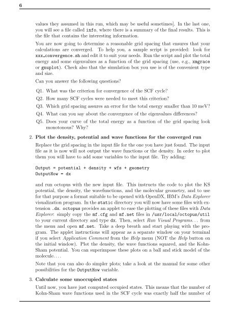
6<br />
values <strong>the</strong>y assumed in this run, which may be useful sometimes]. In <strong>the</strong> last one,<br />
you will see a file called info, where <strong>the</strong>re is a summary of <strong>the</strong> final results. This is<br />
<strong>the</strong> file that contains <strong>the</strong> interesting information.<br />
You are now going <strong>to</strong> determine a reasonable grid spacing that ensures that your<br />
calculations are converged. To help you, a sample script is provided: look for<br />
xxx convergence.sh and edit it <strong>to</strong> suit your needs. Run <strong>the</strong> script and plot <strong>the</strong> <strong>to</strong>tal<br />
energy and some eigenvalues as a function of <strong>the</strong> grid spacing (use, e.g., xmgrace<br />
or gnuplot). Check also that <strong>the</strong> simulation box you use is of <strong>the</strong> convenient type<br />
and size.<br />
Can you answer <strong>the</strong> following questions<br />
Q1. What was <strong>the</strong> criterion for convergence of <strong>the</strong> SCF cycle<br />
Q2. How many SCF cycles were needed <strong>to</strong> meet this criterion<br />
Q3. Which grid spacing assures an error for <strong>the</strong> <strong>to</strong>tal energy smaller than 10 meV<br />
Q4. What can you say about <strong>the</strong> convergence of <strong>the</strong> eigenvalues differences<br />
Q5. Does your curve of <strong>the</strong> <strong>to</strong>tal energy as a function of <strong>the</strong> grid spacing look<br />
mono<strong>to</strong>nous Why<br />
2. Plot <strong>the</strong> density, potential and wave functions for <strong>the</strong> converged run<br />
Replace <strong>the</strong> grid spacing in <strong>the</strong> input file for <strong>the</strong> one you have just found. The input<br />
file as it is now will not output <strong>the</strong> wave functions or <strong>the</strong> density. In order <strong>to</strong> plot<br />
<strong>the</strong>m you will have <strong>to</strong> add some variables <strong>to</strong> <strong>the</strong> input file. Try adding:<br />
Output = potential + density + wfs + geometry<br />
OutputHow = dx<br />
and run oc<strong>to</strong>pus with <strong>the</strong> new input file. This instructs <strong>the</strong> <strong>code</strong> <strong>to</strong> plot <strong>the</strong> KS<br />
potential, <strong>the</strong> density, <strong>the</strong> wavefunctions, and <strong>the</strong> molecular geometry, and <strong>to</strong> use<br />
for that purpose a format suitable <strong>to</strong> be opened with OpenDX, IBM’s Data Explorer<br />
visualization program. In <strong>the</strong>static direc<strong>to</strong>ry you will now have some files with extension<br />
.dx. oc<strong>to</strong>pus provides an applet <strong>to</strong> ease <strong>the</strong> plotting of <strong>the</strong>se files with Data<br />
Explorer: simply copy <strong>the</strong> mf.cfg and mf.net files in /usr/local/oc<strong>to</strong>pus/util<br />
<strong>to</strong> your current direc<strong>to</strong>ry and type dx. Then, select Run Visual Programs... from<br />
<strong>the</strong> menu and open mf.net. Take a deep breath and start playing with <strong>the</strong> program.<br />
The applet instructions will appear as a separate window on your terminal<br />
if you select Application Comment from <strong>the</strong> Help menu (NOT <strong>the</strong> Help but<strong>to</strong>n on<br />
<strong>the</strong> initial window). Plot <strong>the</strong> density, <strong>the</strong> wave functions squared, and <strong>the</strong> Kohn-<br />
Sham potential. You can superimpose <strong>the</strong>se plots on a ball and stick model of <strong>the</strong><br />
molecule....<br />
Note that you can also do simpler plots; take a look at <strong>the</strong> manual for some o<strong>the</strong>r<br />
possibilities for <strong>the</strong> OutputHow variable.<br />
3. Calculate some unoccupied states<br />
Until now, you have just computed occupied states. This means that <strong>the</strong> number of<br />
Kohn-Sham wave functions used in <strong>the</strong> SCF cycle was exactly half <strong>the</strong> number of