Introduction to the octopus code - TDDFT.org

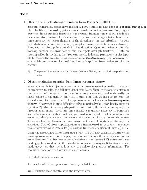
section 3. Second session 11
Tasks
1. Obtain the dipole strength function from Friday’s TDDFT run
Your run from Friday should have finished by now. You should have a bigtd.general/multipoles
file. This file will be used by yet another external tool, oct-cross-section, to generate
the dipole strength function of the system. Running this tool will produce a
cross section vector file with several columns: the energy (first column) and
three cross section tensor elements in the direction of the perturbation. (As your
perturbation is in one direction only, you get just one cross section tensor element).
Also, you get the dipole strength in that direction (Question: what is the relationship
between the cross section and the dipole strength function) Units are
those specified in the input file. You can use the following parameters in the input
file to control the calculation of the spectrum: SpecMaxEnergy (the maximum energy
which you want to plot) and SpecEnergyStep (the discretization step for the
energy).
Q1. Compare this spectrum with the one obtained Friday and with the experimental
results.
2. Obtain excitation energies from linear response theory
When a molecule is subject to a weak external time-dependent potential, it may not
be necessary to solve the full time-dependent Kohn-Sham equations to determine
the behavior of the system: perturbation theory allows us to calculate easily the
linear change of the density, and that in turn is all that we need to get, e.g., the
optical absorption spectrum. This approximation is known as linear-response
theory. However, it is quite difficult to solve numerically the linear density response
equation [2], which is an integral equation that requires the non-interacting response
function as an input. To obtain this quantity it is usually necessary to perform a
summation over all states, both occupied and unoccupied. Such summations are
sometimes slowly convergent and require the inclusion of many unoccupied states.
There are however frameworks that circumvent the full solution of the response
equation. Two of these approximations are implemented in octopus: the singlepole
approximation of Petersilka [13] and the full matrix solution of Casida [14, 15].
Using the unoccupied states calculated Friday you will now generate spectra within
these approximations. For this purpose, you need to do a third octopus run in the
same directory [the first one is the calculation of the occupied KS states with run
mode gs; the second run is the calculation of some unoccupied KS states with run
mode unocc], so that the code is able to retrieve the previous information. The
necessary mode for this third run is called casida:
CalculationMode = casida
The results will show up in some directory called linear.
Q2. Compare these spectra with the previous ones.