Introduction to the octopus code - TDDFT.org

More documents

Recommendations

Info

12 Q3. The results of a LR-TDDFT calculation such as the one that you have just performed depend on the number of unoccupied KS states included in the calculation. Ideally all of them should be included. You may see how the results converge to the exact numbers upon inclusion of more unoccupied KS states. 3. Obtain cross section and polarizability from linear response theory Another approach to linear response theory is implemented in Octopus. This method is based in the Density Functional Perturbation Theory, where the linear perturbations of the Kohn-Sham orbitals and the density are calculated. The advantage of this method with respect to the previous ones is that response for any desired frequency can be obtained and that the unoccupied states are not needed. The disadvantage is that this approach is much slower (at least for the moment) if we want to calculate a full spectrum or the excitation energies. In this case we will only calculate the static polarizability (ω = 0) but response for any frequency can be calculated (including excitation energies). First of all we have to use the run mode pol lr: CalculationMode = pol_lr The energy of the excitation is given by the PolFreqs block, in this case we will only give one frequency: %PolFreqs 1 | 0.0 % More frequencies can be given by adding more rows to this block. To specify a range of values you have to put three numbers, the first number is the number of frequencies in the interval, the following two numbers are the lower and upper limits of the interval. To obtain absorption spectra it is necessary to give a small complex part to the frequency. This is specified by the PolEta variable. In this case we will use a value of 0.1 eV: PolEta = 0.1 Now execute octopus. For this run you only need the result of a ground state calculation. This will take some minutes. At the end of the run, in the linear/ directory you will find two files, alpha and cross section tensor. The first file contains the polarizability tensor α ij (−ω, ω) for each frequency and the second one the cross section tensor.
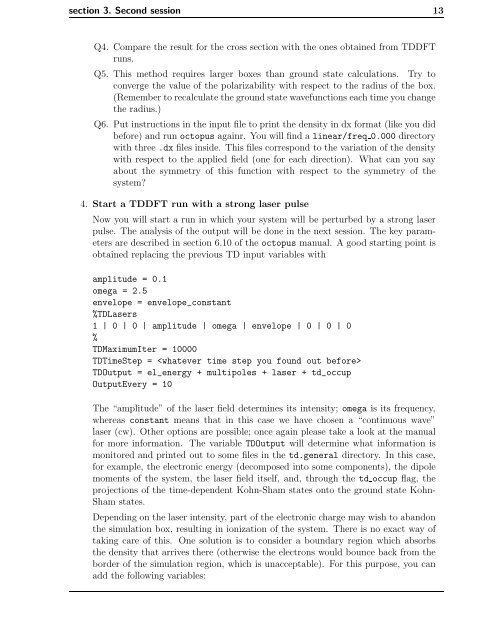
section 3. Second session 13 Q4. Compare the result for the cross section with the ones obtained from TDDFT runs. Q5. This method requires larger boxes than ground state calculations. Try to converge the value of the polarizability with respect to the radius of the box. (Remember to recalculate the ground state wavefunctions each time you change the radius.) Q6. Put instructions in the input file to print the density in dx format (like you did before) and run octopus againr. You will find a linear/freq 0.000 directory with three .dx files inside. This files correspond to the variation of the density with respect to the applied field (one for each direction). What can you say about the symmetry of this function with respect to the symmetry of the system 4. Start a TDDFT run with a strong laser pulse Now you will start a run in which your system will be perturbed by a strong laser pulse. The analysis of the output will be done in the next session. The key parameters are described in section 6.10 of the octopus manual. A good starting point is obtained replacing the previous TD input variables with amplitude = 0.1 omega = 2.5 envelope = envelope_constant %TDLasers 1 | 0 | 0 | amplitude | omega | envelope | 0 | 0 | 0 % TDMaximumIter = 10000 TDTimeStep = TDOutput = el_energy + multipoles + laser + td_occup OutputEvery = 10 The “amplitude” of the laser field determines its intensity; omega is its frequency, whereas constant means that in this case we have chosen a “continuous wave” laser (cw). Other options are possible; once again please take a look at the manual for more information. The variable TDOutput will determine what information is monitored and printed out to some files in the td.general directory. In this case, for example, the electronic energy (decomposed into some components), the dipole moments of the system, the laser field itself, and, through the td occup flag, the projections of the time-dependent Kohn-Sham states onto the ground state Kohn- Sham states. Depending on the laser intensity, part of the electronic charge may wish to abandon the simulation box, resulting in ionization of the system. There is no exact way of taking care of this. One solution is to consider a boundary region which absorbs the density that arrives there (otherwise the electrons would bounce back from the border of the simulation region, which is unacceptable). For this purpose, you can add the following variables:
Page 1 and 2: Practical session octopus I-II Intr
Page 3 and 4: section 1. Introduction 3 The time-
Page 5 and 6: section 2. First session 5 http://w
Page 7 and 8: section 2. First session 7 valence
Page 9 and 10: section 2. First session 9 Note tha
Page 11: section 3. Second session 11 Tasks
Page 15: REFERENCES, COMMENTS, ETC. 15 Refer

Introduction to the octopus code - TDDFT.org

You also want an ePaper? Increase the reach of your titles

Delete template?

Save as template?