Introduction to the octopus code - TDDFT.org

14
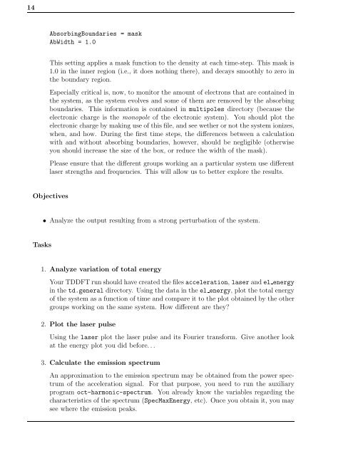
AbsorbingBoundaries = mask
AbWidth = 1.0
This setting applies a mask function to the density at each time-step. This mask is
1.0 in the inner region (i.e., it does nothing there), and decays smoothly to zero in
the boundary region.
Especially critical is, now, to monitor the amount of electrons that are contained in
the system, as the system evolves and some of them are removed by the absorbing
boundaries. This information is contained in multipoles directory (because the
electronic charge is the monopole of the electronic system). You should plot the
electronic charge by making use of this file, and see wether or not the system ionizes,
when, and how. During the first time steps, the differences between a calculation
with and without absorbing boundaries, however, should be negligible (otherwise
you should increase the size of the box, or reduce the width of the mask).
Please ensure that the different groups working an a particular system use different
laser strengths and frequencies. This will allow us to better explore the results.
Objectives
• Analyze the output resulting from a strong perturbation of the system.
Tasks
1. Analyze variation of total energy
Your TDDFT run should have created the filesacceleration, laser andel energy
in the td.general directory. Using the data in the el energy, plot the total energy
of the system as a function of time and compare it to the plot obtained by the other
groups working on the same system. How different are they
2. Plot the laser pulse
Using the laser plot the laser pulse and its Fourier transform. Give another look
at the energy plot you did before...
3. Calculate the emission spectrum
An approximation to the emission spectrum may be obtained from the power spectrum
of the acceleration signal. For that purpose, you need to run the auxiliary
program oct-harmonic-spectrum. You already know the variables regarding the
characteristics of the spectrum (SpecMaxEnergy, etc). Once you obtain it, you may
see where the emission peaks.