Oceanographic Modelling of Jurien Bay, Western Australia
Oceanographic Modelling of Jurien Bay, Western Australia
Oceanographic Modelling of Jurien Bay, Western Australia
- No tags were found...

Create successful ePaper yourself
Turn your PDF publications into a flip-book with our unique Google optimized e-Paper software.
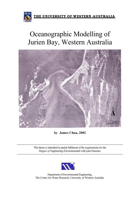
THE UNIVERSITY OF WESTERN AUSTRALIA<strong>Oceanographic</strong> <strong>Modelling</strong> <strong>of</strong><strong>Jurien</strong> <strong>Bay</strong>, <strong>Western</strong> <strong>Australia</strong>by James Chua, 2002----------------------------------------------------------------------------------------------------------------This thesis is submitted in partial fulfilment <strong>of</strong> the requirements for theDegree <strong>of</strong> Engineering (Environmental) with joint Honours.----------------------------------------------------------------------------------------------------------------Department <strong>of</strong> Environmental Engineering,The Centre for Water Research, University <strong>of</strong> <strong>Western</strong> <strong>Australia</strong>.
<strong>Oceanographic</strong> <strong>Modelling</strong> <strong>of</strong> <strong>Jurien</strong> <strong>Bay</strong>AcknowledgementsACKNOWLEDGEMENTSJMJ † Totus TuusFirst and foremost I must thank the CWR and all its crew members for the undergraduatesupport and for this degree. It has be a privilege to work with all <strong>of</strong> you.This thesis would not have been possible without the project and the supervisor and theguidance from Chari, for his expertise and knowledge.In particular, I must thank Emma Rose for the constant support; keeping me on track andsteering me along the straight and narrow.For my fellow undergraduate students <strong>of</strong> 2002 for the frolic-filled five years, memorable,crazy, and all <strong>of</strong> the other words that could possibly describe what we went through… allnighters,stress, and the inexplicable joy <strong>of</strong> handing this in.Most importantly, the light at the end <strong>of</strong> the tunnel, the light that pierce though the darknessand the darkness could not over come it. I would like to thank Dominus et Deus et Omnia myLord and God Jesus Christ, and His blessed mother for the source <strong>of</strong> inspiration and dailystrength. I’d like to acknowledge my guardian angel and my two patron saints, St. Agatha andSt. Aloysius for the lamp for my feet and the guide for my path.This thesis is dedicated to my parents for their sacrifice and giving me the opportunities inmy life.i J. Chua, Centre for Water Research (2002)
<strong>Oceanographic</strong> <strong>Modelling</strong> <strong>of</strong> <strong>Jurien</strong> <strong>Bay</strong>AbstractABSTRACT<strong>Jurien</strong> <strong>Bay</strong>, <strong>Western</strong> <strong>Australia</strong> is a unique a marine environment located in a transitional zone<strong>of</strong> overlapping tropical and temperate flora and fauna. The precious ecological heritagevalues, naturally requires protection. Concerns about the influence <strong>of</strong> proposed urbandevelopment upon ecological heritage values in the bay have motivated this study into thenearshore flushing characteristics <strong>of</strong> <strong>Jurien</strong> <strong>Bay</strong>. A Marine Park classification has also beenproposed to the marine environment adjacent to the development area.<strong>Jurien</strong> <strong>Bay</strong> is a wind dominated lagoonal system. The nearshore circulation patterns andflushing characteristics are investigated using a 3D hydrodynamic model (HAMSOM).Winter field data, collected using an ADCP, was used to validate the model. The field surveyindicates that winds dominating the general coastal circulation pattern.Flushing times using constructed hypothetical meteorological records modelling 12 hourlydaytime regimes consecutively for spring/summer, autumn and winter. Flushing times duringsummer are estimated to be 1.5 to 6 days, whilst during the winter months flushing times arefound to be 2 to 5 days, and 4 days in autumn.Particle tracks are estimated to exit the study area within 2 to 3 days during summer, 2 to 4days during winter, and 3 to 5 days during autumn. The particle tracking highlighted FavoriteLagoon as a possible problematic area due to recirculation within the bay during winter;particles washed up along the shore under a propagating storm front from the northwest; andduring autumn longshore currents causing particles to be trapped behind the headland atNorth Head.Increased flows and loadings under the post-development secenario was quantified.<strong>Modelling</strong> <strong>of</strong> the groundwater discharge and total nitrogen loadings for a summer baselineand post-development scenario predicts negligible changes in water quality.ii J. Chua, Centre for Water Research (2002)
<strong>Oceanographic</strong> <strong>Modelling</strong> <strong>of</strong> <strong>Jurien</strong> <strong>Bay</strong>CONTENTS PAGEContents PageACKNOWLEDGEMENTS ........................................................................................................ IABSTRACT...............................................................................................................................IICONTENTS PAGE ................................................................................................................. IIILIST OF FIGURES................................................................................................................... VLIST OF TABLES.................................................................................................................. VII1.0 INTRODUCTION ............................................................................................................11.1 RESEARCH RATIONALE.................................................................................................... 22.0 ENVIRONMENTAL SETTINGS.....................................................................................52.1 COASTAL GEOMORPHOLOGY............................................................................................ 52.2 BATHYMETRY................................................................................................................. 62.3 ECOLOGICAL SIGNIFICANCE........................................................................................... 102.4 CLIMATIC SETTING........................................................................................................ 112.4.1 Synoptic Weather Pattern........................................................................................112.4.2 Atmospheric Temperature.......................................................................................132.4.3 Precipitation ..........................................................................................................142.4.4 Winds ....................................................................................................................142.4.4.1 Summer Season................................................................................................... 152.4.4.1.1. Sea breeze .................................................................................................... 152.4.4.2 Winter Season..................................................................................................... 162.4.4.2.1. Storm Events ................................................................................................ 162.4.4.3 Autumn Season ................................................................................................... 172.4.4.3.1. Periods <strong>of</strong> Calm ............................................................................................ 172.4.5 Climate Change......................................................................................................182.5 SURFACE AND SUBSURFACE FLOWS................................................................................ 192.5.1 Hill River...............................................................................................................192.5.1.1 Hill River Water Quality...................................................................................... 212.5.2 Groundwater..........................................................................................................212.5.2.1 Groundwater Water Quality ................................................................................. 232.5.3 Water Quality Within <strong>Jurien</strong> <strong>Bay</strong>.............................................................................243.0 CULTURAL SETTING..................................................................................................253.1 MARINE-BASED INDUSTRIES.......................................................................................... 253.2 RECREATIONAL ACTIVITIES ........................................................................................... 264.0 OCEANOGRAPHIC SETTINGS...................................................................................274.1 REGIONAL CIRCULATION ............................................................................................... 274.1.1 Leeuwin Current.....................................................................................................274.1.2 Capes Current........................................................................................................294.1.3 Continental Shelf Waves..........................................................................................294.2 BAROTROPIC FORCING................................................................................................... 304.2.1 Tides......................................................................................................................314.2.1.1 Tidal forces at <strong>Jurien</strong> <strong>Bay</strong> .................................................................................... 314.2.2 Wave Climate.........................................................................................................344.2.2.1 Wind Stresses ..................................................................................................... 354.2.3 Wave Pumping .......................................................................................................364.2.4 Topographic gyres..................................................................................................384.2.5 Coriolis Force, Rossby Number and Ekman Veering.................................................394.3 BAROCLINIC FORCING.................................................................................................... 41iii J. Chua, Centre for Water Research (2002)
<strong>Oceanographic</strong> <strong>Modelling</strong> <strong>of</strong> <strong>Jurien</strong> <strong>Bay</strong>Contents Page4.3.1 Atmospheric Pressure Variations.............................................................................414.3.2 Sea Temperature ....................................................................................................424.3.3 Stratification ..........................................................................................................424.3.4 Seiches...................................................................................................................444.3.5 Baroclinic circulation .............................................................................................454.4 FLUSHING ..................................................................................................................... 464.4.1 Effects <strong>of</strong> Topography .............................................................................................465.0 METHODOLOGY .........................................................................................................485.1 FIELD STUDY ................................................................................................................ 485.1.1 Acoustic Doppler Current Pr<strong>of</strong>iler...........................................................................485.2 NUMERICAL MODELING................................................................................................. 495.2.1 The Fundamental Equations....................................................................................505.2.2 HAMburg Shelf Ocean Model (HAMSOM)...............................................................515.3 MODEL CALIBRATION.................................................................................................... 525.3.1 Bathymetric Digitisation.........................................................................................525.3.2 Simulation Timesteps..............................................................................................535.3.3 Model Forcing Data ...............................................................................................535.4 WIND REGIMES ............................................................................................................. 545.5 FLUSHING TIME............................................................................................................. 555.6 PARTICLE TRACKING MODULE....................................................................................... 575.7 GROUNDWATER DISCHARGE.......................................................................................... 586.0 RESULTS.......................................................................................................................596.1 FIELD RESULTS ............................................................................................................. 596.2 MODEL SIMULATIONS.................................................................................................... 636.2.1 Seasonal Flushing Times.........................................................................................636.2.1.1 Spring/Summer ................................................................................................... 636.2.1.2 Winter ................................................................................................................ 656.2.1.3 Autumn .............................................................................................................. 676.2.2 Particle Tracking Module........................................................................................686.2.2.1 Spring/Summer ................................................................................................... 696.2.2.2 Winter ................................................................................................................ 706.2.2.3 Autumn .............................................................................................................. 726.2.3 Groundwater Discharge..........................................................................................736.2.3.1 Total Nitrogen Levels .......................................................................................... 746.3 HILL RIVER DISCHARGE ................................................................................................ 767.0 DISCUSSION.................................................................................................................777.1 HYDRODYNAMICS IN JURIEN BAY .................................................................................. 777.1.1 Field Survey...........................................................................................................787.1.2 Summer..................................................................................................................797.1.3 Winter....................................................................................................................807.1.4 Autumn ..................................................................................................................807.2 GROUNDWATER INTERACTION....................................................................................... 817.3 HILL RIVER INTERACTION.............................................................................................. 827.4 WATER QUALITY OF JURIEN BAY................................................................................... 828.0 CONCLUSION...............................................................................................................849.0 RECOMMENDATION ..................................................................................................86REFERENCES.........................................................................................................................88APPENDICIES.........................................................................................................................91iv J. Chua, Centre for Water Research (2002)
<strong>Oceanographic</strong> <strong>Modelling</strong> <strong>of</strong> <strong>Jurien</strong> <strong>Bay</strong>List <strong>of</strong> FiguresLIST OF FIGURESFigure 1: MAP OF PROPOSED MARINE PARK & PROPOSED DEVELOPMENT &STUDY AREA (Source: Sanderson, 1997. Study area and proposed development siteadded on.)Figure 2: Bathymetry <strong>of</strong> the coastal waters <strong>of</strong> <strong>Jurien</strong> <strong>Bay</strong>. The study area marked out fromNorth Head to Hill River. (Adapted from D’Adamo & Monty, 1997)Figure 3: Digitalised bathymetry <strong>of</strong> <strong>Jurien</strong> <strong>Bay</strong> using ArcView GIS 3.2a. Left: North view;Right: South view.Figure 4: Typical Summer Synoptic Weather System (Source: BOM, 2002).Figure 5: Typical Winter Synoptic Weather System (Source: BOM, 2002).Figure 6: Mean Monthly Maximum and Minimum Temperatures, calculated using a 31 yearaverage (BOM, 2002). (* from 1970 to 2001).Figure 7: The Mean Monthly Rainfall in <strong>Jurien</strong> <strong>Bay</strong> (BOM, 2002).Figure 8: Rainfall over Hill River Springs Catchment (855 km 2 ). (Source: WRC, 2002)Figure 9: Historical Record <strong>of</strong> Hill River Discharge from 1971 to 2000. (Source: WRC, 2002)Figure 10: Contour plan <strong>of</strong> groundwater flow along the coastline behind <strong>Jurien</strong> <strong>Bay</strong> duringwinter. The distance along the x-axis stretches approximately 13.3km. The lines in blueshows the current baseline flows, the line in red is a predicted value in the scenario <strong>of</strong>future growth in 30 years.Figure 11: Contour plan <strong>of</strong> groundwater flow along the coastline behind <strong>Jurien</strong> <strong>Bay</strong> duringsummer. The distance along the x-axis stretches approximately 13.3km. The lines inblue shows the current baseline flows, the line in red is a predicted value in the scenario<strong>of</strong> future growth in 30 years.Figure 12: Schematic illustration <strong>of</strong> the generation <strong>of</strong> topographic gyres due to the action <strong>of</strong>wind. (Pattiaratchi & Imberger, 1991)Figure 13: Schematic illustration <strong>of</strong> gravitational driven motion due to differential heatingand cooling (Adapted from Pattiaratchi and Inberger, 1992)Figure 14: The Acoustic Doppler Current Pr<strong>of</strong>iler used in the field.Figure 15: The Model Boundary Definition for the Control Volume.v J. Chua, Centre for Water Research (2002)
<strong>Oceanographic</strong> <strong>Modelling</strong> <strong>of</strong> <strong>Jurien</strong> <strong>Bay</strong>List <strong>of</strong> FiguresFigure 16: Feather Diagram <strong>of</strong> the wind and current velocity vectors during the field survey.The wind vector fields (BOM, 2002) correlated with the current vector fields (ADCPresults).Figure 17: North-South and East-West components <strong>of</strong> the currents at ADCP station in EssexLagoon at 8.57metres from the sea bed (top left), 6.57m from the bed (top right), 4.57mfrom the bed (bottom left), and 2.57m from the bed (bottom right).Figure 18: Flushing Estimates for <strong>Jurien</strong> <strong>Bay</strong> during spring/summer. Plot <strong>of</strong> the percentage <strong>of</strong>water flushed, the wind direction, and wind velocity.Figure 19: Flushing Estimates for <strong>Jurien</strong> <strong>Bay</strong> during spring/summer seabreeze. Plot <strong>of</strong> thepercentage <strong>of</strong> water flushed, the wind direction, and wind velocity.Figure 20: Flushing Estimates for <strong>Jurien</strong> <strong>Bay</strong> during winter. Plot <strong>of</strong> the percentage <strong>of</strong> waterflushed, the wind direction, and wind velocity.Figure 21: Flushing Estimates for <strong>Jurien</strong> <strong>Bay</strong> during autumn. Plot <strong>of</strong> the percentage <strong>of</strong> waterflushed, the wind direction, and wind velocity.Figure 22: Particle Tracking Simulations under the spring/summer wind record. The numberson the diagrams are added over the HAMSOM output indicating every 12 hours.Figure 23: Particle Tracking Simulations under the winter wind record. The numbers on thediagrams are added over the HAMSOM output indicating every 12 hours.Figure 24: Particle Tracking Simulations under the autumn wind record. The numbers on thediagrams are added over the HAMSOM output indicating every 12 hours.Figure 25: Groundwater discharge into coastal waters during summer. Baseline scenario tothe left and post-development scenario to the right.Figure 26: Spring/summer modelling <strong>of</strong> the groundwater discharge. Total Nitrogen (TN)concentration distribution along the shoreline shown as grid cells every 50m.Figure 27: Total Nitrogen concentration in the Essex Lagoon over 142 hours <strong>of</strong> modelling forthe post-development scenario.vi J. Chua, Centre for Water Research (2002)
<strong>Oceanographic</strong> <strong>Modelling</strong> <strong>of</strong> <strong>Jurien</strong> <strong>Bay</strong>List <strong>of</strong> TablesLIST OF TABLESTable 1: The Record <strong>of</strong> the average number <strong>of</strong> mid-latitude cyclonic storms along the CentralWest Coast (Source: Sanderson, 1997).Table 2: Total Annual Hill River Discharge from 1971 to 2000 (WRC, 2002).Table 3: Water Quality Parameters in Hill River (Rockwater Consultants, 2002).Table 4: Comparison between the freshwater flows into the coastal waters in <strong>Jurien</strong> <strong>Bay</strong> andPerth coastal waters (Adapted from PCWS, 1995).Table 5: Average Tidal Constituents for the World (Wright, 1995).Table 6: Harmonic Tidal Constituents <strong>of</strong> <strong>Jurien</strong> <strong>Bay</strong>, WA (Source: ANTT, 2002).Table 7: Tidal Levels for <strong>Jurien</strong> <strong>Bay</strong> (ref. to LAT) (Source: ANTT, 2002).Table 8: Percentages <strong>of</strong> average sea and swell for the Central West Coast Region. Acomparison <strong>of</strong> the frequency <strong>of</strong> wave height and direction for each season is given.(taken from Silvester and Mitchell, 1977).Table 9: Characteristic <strong>of</strong> current Speed at <strong>Jurien</strong> during summer and winter. Data wasobtained from an S4 Current Meter deployed 3.5km SSW <strong>of</strong> Island Point. (Source:Sanderson, 1997: 183)Table 10: Characteristic Length Scale and Rossby Number <strong>of</strong> the lagoons in <strong>Jurien</strong> <strong>Bay</strong>.Table 11: Fundamental cross-shore and alongshore seiche periods in <strong>Jurien</strong> <strong>Bay</strong>.Table 12: Summary <strong>of</strong> the time taken for particles to exit study area. The modelling half dayindicates the 12-hour daytime wind data that was used. The third column gives anestimated in whole days under a continuous diurnal wind regime.vii J. Chua, Centre for Water Research (2002)
<strong>Oceanographic</strong> <strong>Modelling</strong> <strong>of</strong> <strong>Jurien</strong> <strong>Bay</strong>Introduction1.0 INTRODUCTIONThe township <strong>of</strong> <strong>Jurien</strong> has a population <strong>of</strong> over 950 residents and is situated some 260kmnorth <strong>of</strong> Perth on the West <strong>Australia</strong>n coast. Offshore to the coast is <strong>Australia</strong>’s longestcontinuous limestone reef system which extends 300km from Dongara to Hillarys. <strong>Jurien</strong> <strong>Bay</strong>is the hub <strong>of</strong> the rock lobster industry in <strong>Western</strong> <strong>Australia</strong>, worth around $300 million, and isalso an important tourist centre.A visible transition in marine flora and fauna occurs from the tropical north to the temperatesouth along the west coast. <strong>Jurien</strong> <strong>Bay</strong> lies within this transitory zone making it a very uniqueenvironment. The <strong>of</strong>fshore environment <strong>of</strong> <strong>Jurien</strong> <strong>Bay</strong> features a complex bathymetry <strong>of</strong>shallow limestone reefs with rocky outcrops, emergent islands and sheltered lagoons cradlinga rich potpourri <strong>of</strong> tropical and temperate marine life with a number <strong>of</strong> endemic species (Calm,1998). It was suggested by the Wilson Report (Calm, 1994) that the biogeographical areaencompassing <strong>Jurien</strong> <strong>Bay</strong> (roughly 26km long) is representative <strong>of</strong> the Central West Coastand thus worthy <strong>of</strong> protection as a multiple purpose marine reserve.The high conservation nature values in <strong>Jurien</strong> <strong>Bay</strong> including some unique and distinct coastaltype, its Class “A” Nature Reserve Islands, some endermic fauna species totalling to arepresentative reserve system. A marine reserve classification for <strong>Jurien</strong> <strong>Bay</strong> will bebeneficial to the local community in several ways:1. to ensure the long-term survival and management <strong>of</strong> the marine environment,2. the protection <strong>of</strong> marine species, their habitats and their long-term survival.3. a resource for education, recreation and tourism programs (CALM, 1994).The multiple-use <strong>of</strong> a marine reserve will provide a framework for both socio-economic andbiological interest by allow commercial activities, such as fishing, aquaculture and petroleumexploration and production while at the same time set some parameters around themanagement <strong>of</strong> these activities to ensure a continual sustainable use (CALM Act 1984).1 J. Chua, Centre for Water Research (2002)
<strong>Oceanographic</strong> <strong>Modelling</strong> <strong>of</strong> <strong>Jurien</strong> <strong>Bay</strong>IntroductionRecent proposals have been made to develop the land around <strong>Jurien</strong> <strong>Bay</strong>, making the need tosanction the area as a Marine Park more imperative. The escalation <strong>of</strong> eutrophic waterwaysworldwide in recent years has intensified the awareness <strong>of</strong> the vulnerability <strong>of</strong> coastalenvironments to threats <strong>of</strong> contamination, sedimentation and destruction. Examples in<strong>Western</strong> <strong>Australia</strong> includes the previous Peel-Harvey system, Cockburn Sound and isolatedincidents <strong>of</strong> algal blooms in the Swan River (SOMER, 1995). 1 The need to address thehydrodynamic regime <strong>of</strong> the nearshore environment warrants this study.1.1 Research RationalePrevious hydrodynamic studies in <strong>Jurien</strong> <strong>Bay</strong> have been inconclusive with respect to thecurrent circulation and flushing regimes within the nearshore zone. Pang (1997) modelled the<strong>Jurien</strong> area using the HAMSOM model (D’Adamo and Monty, 1995) in a relatively largeregional scale domain, using a 250m grid size. Using typical sea-breeze conditions the modelwas able to describe the directional characteristics <strong>of</strong> broad-scale current patterns withreasonable accuracy over Sandy Point and Cervantes. The model developed by Pang (1997)applied a constant wind regime from SW, SE, NE and NW directions. The model appeared toover-predict the average current speeds by a factor <strong>of</strong> two and over-predicted the nearbedvelocities in the deep basins by a factor <strong>of</strong> 10 (D’Adamo & Monty, 1997).This study attempts to provide a sufficient understanding <strong>of</strong> the circulation patterns andflushing characteristics that will be required for the planning and management <strong>of</strong> the growthexpected in the future with the implementation <strong>of</strong> the proposed development by ArdrossEstate. This report will also add to the technical understanding <strong>of</strong> oceanographic informationfor the proposed <strong>Jurien</strong> <strong>Bay</strong> Marine Reserve, as well as <strong>of</strong> benefit to the management <strong>of</strong>commercial and recreational marine activity. The study area is represented as a rectangularregion (13.3km by 24.5km) covering an area <strong>of</strong> 326.5 km 2 . The study area shown on the mapin Figure 1 is defined according to the boundaries 114°55′00″E to 115°03′30″E longitudes;and latitudes <strong>of</strong> 29°12′06″S to 31°25′92″S.1 Cockburn Sound has lost approximately 80% <strong>of</strong> its seagrass meadows. Economic cost toreducing eutrophic systems have added up to $170 million in Cockburn Sound and $50 million forthe Dawesville Cut in Peel-Harvey (SOMER, 1995).2 J. Chua, Centre for Water Research (2002)
<strong>Oceanographic</strong> <strong>Modelling</strong> <strong>of</strong> <strong>Jurien</strong> <strong>Bay</strong>IntroductionThe modelling <strong>of</strong> flushing times and current patterns will aid in the assessment <strong>of</strong> the possiblefate and transport <strong>of</strong> contamination within the nearshore waters. <strong>Modelling</strong> the postdevelopmentscenario will provide an understanding to the impacts <strong>of</strong> the increase in nutrientloading in the groundwater discharge. <strong>Modelling</strong> will also provide better knowledge andunderstanding to ensure continual protection <strong>of</strong> the coastal environmental and biologicalsignificance by the authorities and sustainability <strong>of</strong> the area.In order to achieve this, the study objectives are:• A literature review to the physical processes <strong>of</strong> <strong>Jurien</strong> <strong>Bay</strong> and to investigate thehydrodynamics and flushing regimes. Specifically to make way for the development<strong>of</strong> a desktop model to estimate the effects <strong>of</strong> groundwater inflows and hypotheticalincreases in nutrient loading.• The use <strong>of</strong> a three-dimensional, hydrodynamic model will help determine:∗ the flushing characteristics in vicinity <strong>of</strong> <strong>Jurien</strong> <strong>Bay</strong> with particular regard to theexchange <strong>of</strong> coastal waters with <strong>of</strong>fshore waters for each season.∗ the particle movements on the surface under certain wind condition typical to eachseason.∗ the incorporation <strong>of</strong> groundwater flows for a baseline and post-developmentscenario to assess the effects <strong>of</strong> an increase in nutrient influxes on the waterquality.3 J. Chua, Centre for Water Research (2002)
<strong>Oceanographic</strong> <strong>Modelling</strong> <strong>of</strong> <strong>Jurien</strong> <strong>Bay</strong>IntroductionFigure 1: MAP OF PROPOSED MARINE PARK & PROPOSED DEVELOPMENT &STUDY AREA (Source: Sanderson, 1997. Study area and proposed development siteadded on.4 J. Chua, Centre for Water Research (2002)
<strong>Oceanographic</strong> <strong>Modelling</strong> <strong>of</strong> <strong>Jurien</strong> <strong>Bay</strong>Environmental Settings2.0 ENVIRONMENTAL SETTINGSThis chapter provides an overview <strong>of</strong> the environmental setting <strong>of</strong> <strong>Jurien</strong> <strong>Bay</strong>. The geography<strong>of</strong> the coastal zone will be examined and the regional climate <strong>of</strong> the Central West Coast andthe relevant statistical meteorological information will also be discussed in this chapter.The coastal waters <strong>of</strong> <strong>Jurien</strong> <strong>Bay</strong> is oligotrophic. The seagrass meadows among otherbiological species are highly nutrient-sensitive and can be vulnerable to eutrophication andsedimentation This chapter will also cover the ecological significance and surface andsubsurface flows that may be presented as potential threats to water quality issues.2.1 Coastal GeomorphologyThe coastline stretches some two thousand kilometres <strong>of</strong> long sandy beaches, dominated bybioclastic carbonate and quartz sediments, composed <strong>of</strong> the skeletal remains <strong>of</strong> marineorganisms. The shoreline <strong>of</strong> <strong>Jurien</strong> <strong>Bay</strong> is generally aligned in the north-south direction. Thecoast consists <strong>of</strong> arcuate beaches falling back on salient cuspate foredune plains (Sanderson,1997). The yellow sands forming the sand dunes are composed <strong>of</strong> yellow quartz which sits onthe Tamala limestone formation assumed to have deposited in the Quaternary period reachingto 8km inland in certain areas (CALM, 1998).<strong>Jurien</strong> <strong>Bay</strong> has been formed as a semi-enclosed basin characterised by a chain <strong>of</strong> limestonereef parallel to the coastline, fringing several sheltered lagoonal pools in the nearshore region(Sanderson, 1997). The nearshore features an array <strong>of</strong> rocky outcrops and emergent islands(CALM, 1994). The Central West Coast is generally considered microtidal, with a relativelyhigh-energy wave system, although <strong>Jurien</strong> is a low energy, reflective environment due to theprotection <strong>of</strong> the reef chain <strong>of</strong>fshore (Elliot, pers comm, 2002).The continental shelf in the region is very narrow, with occasional limestone cliffs andheadlands, <strong>of</strong>fshore limestone island and reef complexes (Sanderson, 1997). Several mediumsized limestone islands (Sandland, Favorite, Boullanger, Whitlock, Escape, Cervantes) forman interbarrier zone which has developed as an embayment. Two deep inshore basinsenclosed by the islands, exist north and south <strong>of</strong> Island Point.5 J. Chua, Centre for Water Research (2002)
<strong>Oceanographic</strong> <strong>Modelling</strong> <strong>of</strong> <strong>Jurien</strong> <strong>Bay</strong>Environmental SettingsRocky limestone platforms are a significant feature <strong>of</strong> the West Coast (CALM, 1994). Severalrocky headlands composed <strong>of</strong> Tamala Limestone lie along the coast including North Head tothe north and a prominent sandy tombola at Island Point (CALM, 1994). Several sedimentaryprocesses composed <strong>of</strong> shallow sand banks, spits or tombolas connects the nearshore islandsand reefs to the mainland. The sand promontory at Island Point was developed behind theprotection <strong>of</strong> Boullanger Island.The morphological features <strong>of</strong> the forelands, salients and tombolos <strong>of</strong> the central west coastare formed by the combination <strong>of</strong> the prevailing coastal conditions and nearshore topography.While past climate trends, storm events and the shift <strong>of</strong> sediment supply also play a major role.Unlike the south coast, the central west coast owes much <strong>of</strong> its morphological development to<strong>of</strong>fshore obstacles (Sanderson, 1997).Long-term weather patterns, variations and storm effects have played a significant factor inthe shore erosion and morphology. The changes in the storm tracks, frequency and intensityconstitute a major factor in much <strong>of</strong> the coastal change and stability (Thom, 1978; Sanderson,1997).2.2 BathymetryThe bathymetry <strong>of</strong> <strong>Jurien</strong> <strong>Bay</strong> is complex with variable depth patches and a chain <strong>of</strong> unevenlimestone reef outcropping structures. The limestone reef systems has an average depth <strong>of</strong> 1to 2 metres with some rocks being exposed during low tide periods. Waves break over thereef under moderate to rough wave conditions (CALM, 1994). The reef structure runs parallelto the shore and protects the inshore lagoonal region with an average depth <strong>of</strong> 5 to 6 metres.The shelf is 6km from the coast. <strong>Jurien</strong> <strong>Bay</strong> has a gentle seaward sloping seabed, with depthsranging from 1 to 2 metres near the coast to 20 metres around breakwaters. The reef chain isroughly 4km from the shore and runs parallel to the shoreline around 10km north to southfrom Essex Rocks to Favourite Island with several island and rocky outcrops. Favorite Islandis approximately 500m long, Boullanger Island is approximately 2km by 2km, and EscapeIsland. is 1km long.6 J. Chua, Centre for Water Research (2002)
<strong>Oceanographic</strong> <strong>Modelling</strong> <strong>of</strong> <strong>Jurien</strong> <strong>Bay</strong>Environmental SettingsThe series <strong>of</strong> elongated basins exist between the reefs and the shore reaching depths <strong>of</strong> 12 to15 m and appear to have restricted bottom circulation to the open sea (CALM, 1994). Figure 2shows the two more prominent pools are Favorite and Essex Lagoon will be studied moreclosely in this report. The first <strong>of</strong> this pools lies between North Head to the north and IslandPoint to the south. The second lies south <strong>of</strong> Island Point and Hill River.Favorite Lagoon is a deep semi-enclosed basin, encompassed by limestone outcrops to thenorth and runs 8km to Boullanger Island in the south. It spans 5km wide from the coast to thereef line adjoining Seaward Ledge and The Boomer, with intermitted sills and reefs fromFavorite Island to north <strong>of</strong> the <strong>Jurien</strong> <strong>Bay</strong> marina. The pool has a mean depth <strong>of</strong> 10 metreswith a maximum depth <strong>of</strong> 14 metres just south <strong>of</strong> North Head. The basin has a volume <strong>of</strong>approximately 4 x10 8 m 3 .Essex Lagoon lies 3km south <strong>of</strong> Island Point, adjacent to Essex Rocks. Several aquaculturecages are currently located north <strong>of</strong> the pool. The lagoon is semi-enclosed with protection bythe <strong>of</strong>fshore reefs and Boullanger Island to the north. The lagoon is 4km long by 4km widefrom the shore to the <strong>of</strong>fshore reefs. The mean depth is 10m with a maximum depth <strong>of</strong> 13m.The volume <strong>of</strong> the pool is roughly 1.6 x 10 8 m 3 .Hill River is a small riverine estuary which runs approximately 10km south <strong>of</strong> the <strong>Jurien</strong> <strong>Bay</strong>.The estuary mouth is situated adjacent to Essex Lagoon and breaks directly into the lagoon.The river mouth is closed for most <strong>of</strong> the year and only breaks seasonally.Previous hydrodynamic studies <strong>of</strong> the area have adopted a larger regional scale area. Pang(1997) modelled the hydrodynamic regime <strong>of</strong> <strong>Jurien</strong> using a grid size <strong>of</strong> 250m x 250m, fromseveral kilometres north <strong>of</strong> North Head to Cerventes. Inaccuracies including over predictions<strong>of</strong> the current speeds in the surface and nearbed velocities which arose form this model wasattributed on the poor interpolation <strong>of</strong> the complex depth variations (due to the nature <strong>of</strong> thelarge grid sizes) north <strong>of</strong> Island Point.7 J. Chua, Centre for Water Research (2002)
<strong>Oceanographic</strong> <strong>Modelling</strong> <strong>of</strong> <strong>Jurien</strong> <strong>Bay</strong>Environmental SettingsFigure 2: Bathymetry <strong>of</strong> the coastal waters <strong>of</strong> <strong>Jurien</strong> <strong>Bay</strong>. The study area marked outfrom North Head to Hill River. (Adapted from D’Adamo & Monty, 1997)8 J. Chua, Centre for Water Research (2002)
<strong>Oceanographic</strong> <strong>Modelling</strong> <strong>of</strong> <strong>Jurien</strong> <strong>Bay</strong>Environmental SettingsFigure 3: Digitalised bathymetry <strong>of</strong> <strong>Jurien</strong> <strong>Bay</strong> using ArcView GIS 3.2a.Left: North view; Right: South view.This study uses matrix <strong>of</strong> 50m x 50m grid size to better incorporate the complex bottomtopography and to model more accurately the flow and flushing regimes. The study areacovers the coastal waters from North Head to just below Hill River. The modelling gridcovers an area <strong>of</strong> 326.5 km 2 (13.3km wide by 24.5km long).9 J. Chua, Centre for Water Research (2002)
<strong>Oceanographic</strong> <strong>Modelling</strong> <strong>of</strong> <strong>Jurien</strong> <strong>Bay</strong>Environmental Settings2.3 Ecological SignificanceThe Central West Coast (between Carnarvon to Cape Leeuwin) displays a transitional zone <strong>of</strong>rich biological overlap (CALM, 1994). Many <strong>of</strong> the species are believed to be endermic to theWest <strong>Australia</strong>n coast. These includes, the <strong>Western</strong> Rock-Lobster (Panulirus Cygnus) whichis important for its commercial value; and the Dhufish (Glaucosoma hebraicum); along withother conspicuous species like the gastropod Campanile cymbolicum thought to be ‘livingfossils’.The existence <strong>of</strong> this unique marine bioregion is made possible by the continual flow <strong>of</strong>warmer, tropical waters brought down by the Leeuwin Current to the cooler, temperate waters<strong>of</strong>f the south coast <strong>of</strong> <strong>Western</strong> <strong>Australia</strong> (CALM, 1994). Hatcher (1991) discussed extensivelythe importance <strong>of</strong> the Leeuwin Current in sustaining the floral and faunal communities in theCentral West Coast. The Leeuwin Current transports and disperses tropical marine organismsin their larval stages (planktonic), meanwhile maintaining the warm temperatures necessaryfor their survival and growth (PCWS, 1995). As the Leeuwin Current crosses the continentalshelf, larvae may be trapped in eddies behind islands and settle among the nearshore reefs.Kirkman & Walker (1989) revealed 22 species in 9 genera <strong>of</strong> seagrass exist in the West Coastregion, dominating the lagoons and banks behind the protective <strong>of</strong>fshore reefs. Coralcommunities are found in isolated colonies within the sheltered lagoons in <strong>Jurien</strong> <strong>Bay</strong> (CALM,1994). Seagrass meadows play a significant part in the recycling <strong>of</strong> nutrients, providing asource <strong>of</strong> food and habitat for many life forms, including the western rock lobster (CALM,1994).The representation <strong>of</strong> northern and southern species provides a colourful and magnificentspectacle for recreational divers (CALM, 1994). If the adjacent land were to be developed, itis important that these marine communities be protected.10 J. Chua, Centre for Water Research (2002)
<strong>Oceanographic</strong> <strong>Modelling</strong> <strong>of</strong> <strong>Jurien</strong> <strong>Bay</strong>Environmental Settings2.4 Climatic SettingThe Central West Coast exhibits a Mediterranean climate <strong>of</strong> cool wet winters and warm drysummers (Gentilli, 1972). The region is dominated by the seasonal migration anddevelopment <strong>of</strong> eastward moving subtropical high pressure anticyclones both in summer andin winter. The other seasonal phenomenon experienced in <strong>Jurien</strong> is strong local sea breezesystems in summer, periodic storms in winter brought about by the tail <strong>of</strong> the mid-latitudedepressions which pass over much <strong>of</strong> the southwest <strong>of</strong> <strong>Western</strong> <strong>Australia</strong>, and periods <strong>of</strong> calmin autumn (Sanderson, 1997).2.4.1 Synoptic Weather PatternThe most prominent feature <strong>of</strong> the prevailing weather pattern is the subtropical belt <strong>of</strong> highpressure anti-cyclonic cells which are <strong>of</strong> the order <strong>of</strong> 2000km in diameter (Gentilli, 1972).These high pressure cells shift from the east to west, with a period <strong>of</strong> 7 to 10 days, bringingwarm, dry southeasterly to northeasterly winds to west coast much throughout summer andwinter. The variable intensity <strong>of</strong> the anticyclonic system and direction <strong>of</strong> travel will dictatethe magnitude and, direction <strong>of</strong> the winds to <strong>Jurien</strong> <strong>Bay</strong>.Figure 4: Typical Summer Synoptic Weather System (Source: BOM, 2002).11 J. Chua, Centre for Water Research (2002)
<strong>Oceanographic</strong> <strong>Modelling</strong> <strong>of</strong> <strong>Jurien</strong> <strong>Bay</strong>Environmental SettingsThe typical summer synoptic pattern for the months from December to February is shown inthe Figure 4. The subtropical highs are usually located between latitudes <strong>of</strong> 37°S to 38°S(Gentilli, 1972). The summer is warm and dry, with predominant easterlies (CALM, 1998).Low pressure systems to the north coast may initiate some fast moving tropical cycloneswhich may cause storm surges and continental shelf waves down the coast (CALM, 1998).The dominating weather influences on the coastal waters are the sea-breeze in the afternoonand the opposing easterly land-breeze cycle. Another major weather influence is the lowpressure troughs which develops <strong>of</strong>f the west coast from time to time carries cool,southwesterly winds to the coast.Figure 5: Typical Winter Synoptic Weather System (Source: BOM, 2002).The typical winter synoptic pattern for the months <strong>of</strong> June, July and August are shown inFigure 5. The subtropical high pressure cells rises in winter to higher latitudes (29°S to 32°S),than in summer (Gentilli, 1971). This movement allows the passages <strong>of</strong> mid-latitude lowpressuresystems to sweep the in the southwest more periodically. The mid-latitude cyclonesare smaller in diameter and faster moving, crossing the coast every 5 to 7 days and result in12 J. Chua, Centre for Water Research (2002)
<strong>Oceanographic</strong> <strong>Modelling</strong> <strong>of</strong> <strong>Jurien</strong> <strong>Bay</strong>Environmental Settingswesterly cold fronts and periodic precipitation. Cold fronts and gusty winds usuallyaccompany these cyclonic pressure systems, which approach from the northwest to southwestand can generate large swell waves to the coast. Although these winds are strong they areusually short lived (Sanderson, 1997).2.4.2 Atmospheric TemperatureThe highest temperatures occurs during summer with an average maximum temperature <strong>of</strong>30.7°C in February, while the lowest temperatures occurs during winter falling to an averageminimum <strong>of</strong> 9.4°C in August (BOM, 2002). The annual average maximum and minimumtemperatures are 24.7°C and 13.1°C respectively (BOM, 2002). The mild conditions andrelatively small variations are characteristic <strong>of</strong> coastal environments which are affected by themoderating effect <strong>of</strong> water.Monthly Mean Temperatures *Mean daily max. tempMean daily minimum temp.353025Temperature (deg C)20151050Jan Feb Mar Apr May Jun Jul Aug Sep Oct Nov DecMonthsFigure 6: Mean Monthly Maximum and Minimum Temperatures, calculated using a31 year average (BOM, 2002). (* from 1970 to 2001).Air temperatures may have an effect on the baroclinic forces in the bays due to their role inthe heating and cooling processes <strong>of</strong> coastal water bodies. Baroclinic circulation will not beconsidered in this report as they are negligible compared to the strong winds that dominatesthe nearshore circulation at <strong>Jurien</strong> <strong>Bay</strong>.13 J. Chua, Centre for Water Research (2002)
<strong>Oceanographic</strong> <strong>Modelling</strong> <strong>of</strong> <strong>Jurien</strong> <strong>Bay</strong>Environmental Settings2.4.3 PrecipitationThe rainfall is highly seasonal with an average annual rainfall <strong>of</strong> approximately 750 mm (102raindays). The winter months are relatively wet, with the maximum intensity <strong>of</strong> rainfalloccurring in June with an average <strong>of</strong> 300.2 mm (BOM, 2002). Of the total rainfall, 60% fallsbetween June and August, 20% during spring and 15% during autumn. It is usual to for theregion to experience seasonal drought during the summer months, lasting up to four months(CALM, 1998).350Average Monthly Rainfall *5th decile(median) <strong>of</strong>monthlyrainfall - mm3002509th decile <strong>of</strong>monthlyrainfall - mmRainfall (mm)200150100Highestmonthlyrainfall - mmLowestmonthlyrainfall - mm50Meanmonthlyrainfall - mm0Jan Feb Mar Apr May Jun Jul Aug Sep Oct Nov DecTime (month)Figure 7: The Mean Monthly Rainfall in <strong>Jurien</strong> <strong>Bay</strong> (BOM, 2002).(* The data is an average <strong>of</strong> 31 years, from 1975.)2.4.4 WindsThe local wind conditions have a considerable influence on the regional wave climate,affecting both the direction and strength <strong>of</strong> currents and waves. Winds in <strong>Jurien</strong> aredominantly southerly to southwesterly throughout most <strong>of</strong> the year, with a daily diurnal cycleand distinct seasonal variability in the wind pattern. Wind frequency diagrams showing arepresentative month for the seasons <strong>of</strong> spring/summer, autumn and winter at 0900 and 1500are attached in Appendix I.14 J. Chua, Centre for Water Research (2002)
<strong>Oceanographic</strong> <strong>Modelling</strong> <strong>of</strong> <strong>Jurien</strong> <strong>Bay</strong>Environmental SettingsWinds speeds greater than 8.3 ms -1 are strong enough to transport sediments and generatewaves <strong>of</strong> 4 metres or higher (Sanderson, 1997). The wind speed in <strong>Jurien</strong> <strong>Bay</strong> commonlyhave velocities <strong>of</strong> 10 to 11 ms -1 , although the durations are usually less than 12 hours(Sanderson, 1997). These winds usually blow from the south to southwest during summer andnortherly to westerly winds in winter, autumn and spring.2.4.4.1 Summer SeasonThe summer months experiences predominantly strong south to southeasterly winds,sometimes called the southeast trade winds. These easterly winds are brought about by thehigh pressure anticyclonic belt, which moves south and establishes itself through to autumn.The morning winds velocities are typically south southeasterly in the order <strong>of</strong> 5 ms -1 , bringingabout the dominance <strong>of</strong> a northward flow in the shallower waters on the shelf closer to shore(Sanderson, 1997).2.4.4.1.1. Sea breezeSea breeze is a meteorological phenomena which occurs in most coastal regions, resulting inthe circulation <strong>of</strong> winds at diurnal cycles due to the differential heating <strong>of</strong> the land and the sea(Pattiaratchi, et al. 1993). In the <strong>Jurien</strong> region the land-sea breeze cycle is most pronouncedduring the late spring and summer months (CALM, 1998). The sea breeze has a stronginfluence, especially as it superimposes over the regional meteorological pattern.Sea breeze occurs throughout spring, summer, and even autumn dominating the coastal windclimate developing in the late morning through to the afternoons, with wind speeds <strong>of</strong> 10 to15 ms -1 predominantly from the westerly to southwest (CALM, 1998). Current velocity undersea breeze conditions have been measured at 2 to 10 cms -1 near the bottom (at 9 to 11m depth)and 10 to 20 cms -1 at the surface within the lagoons behind <strong>of</strong> the fringing reefs.15 J. Chua, Centre for Water Research (2002)
<strong>Oceanographic</strong> <strong>Modelling</strong> <strong>of</strong> <strong>Jurien</strong> <strong>Bay</strong>Environmental Settings2.4.4.2 Winter SeasonDuring the winter months the wind direction tends to be variable. The rising <strong>of</strong> theanticyclonic belt over <strong>Australia</strong> increases the incidence <strong>of</strong> low-pressure cells from the south tocross the coast. High pressure cells imbedded in the belt produces a dominant northwesterlygale, usually known as the roaring forties (South <strong>Western</strong> Metropolitan Coastal WatersStudies, 1996).Morning winds are usually weak, sporadic and variable. The wind frequency diagram for themonth <strong>of</strong> July in Appendix I, shows a higher frequency <strong>of</strong> wind from the east in the mornings,although <strong>of</strong> low magnitudes. Stronger winds develop in the afternoons are mostly from thenorthwesterly direction.2.4.4.2.1. Storm EventsWinter seasons are characterised by periodical passing <strong>of</strong> extra tropical cyclonic storms fromthe northwest. A storm is defined as wind speeds above 48knots or 25ms -1 recorded at 10mabove the ground on the Beaufort Wind Scale (BOM, 1993). Typical storm events in <strong>Jurien</strong>are unlike the extreme mid-latitude cyclonic storms to the north, but normally closer to gale(=17 ms -1 ) or near gale (=14 ms -1 ) conditions (Laughlin, 1990; cf. Sanderson, 1997), althoughsome literature considers speeds over 30 knots (16 ms -1 ) as storm winds. For the sake <strong>of</strong>simplicity this report will follow the latter.Storm winds initially approach from the north, swinging anticlockwise and strengthening inintensity to the west. As the low-pressure system usually associated with cold fronts traveleastward, the winds shift tending southwesterly and eventually subsiding in intensity with thepassage <strong>of</strong> time. Storm events may last up to 40 hours (SWMCWS, 1996).Table 1: The Record <strong>of</strong> the average number <strong>of</strong> mid-latitude cyclonic storms along theCentral West Coast (Source: Sanderson, 1997).SEASONNUMBER OF STORMSSummer 32Autumn 34Winter 42Spring 22TOTAL 130Annual Average * 9* over 15 years16 J. Chua, Centre for Water Research (2002)
<strong>Oceanographic</strong> <strong>Modelling</strong> <strong>of</strong> <strong>Jurien</strong> <strong>Bay</strong>Environmental SettingsStorm activity can also be associated with cyclones in the NW and east Indian Oceanresulting in wind speeds <strong>of</strong> up to 48knots or 24ms -1 at 10m above MSL.2.4.4.3 Autumn SeasonAutumn is characterised by weak and variable wind fields. During early autumn, tropicalcyclones may occasionally affect the north, bringing relatively strong easterly to northeasterlywinds and heavy rains to <strong>Jurien</strong> (CALM, 1998). Autumn representative wind diagrams <strong>of</strong> themean 9am wind speeds and mean 3pm wind speeds are attached in the in Appendix I.In fine weather mild sea breeze <strong>of</strong> 3.5 to 5 ms -1 may develop in the afternoons. During lateautumn as well as late spring, periods <strong>of</strong> calm are experienced (CALM, 1998).2.4.4.3.1. Periods <strong>of</strong> CalmCooler temperatures during autumn can be insufficient to induce a sea breeze cycle. Thesecalm conditions are common during March and April and may last for up to 2 to 3 days. Winddata collated by the Bureau <strong>of</strong> Meteorology during autumn <strong>of</strong> 2001 and 2002 shows low meanwind velocities.Previous studies have indicated that winds are the dominant forcing on the water circulationpatterns in the lagoons (Sanderson, 1997; D’Adamo & Monty, 1997). Calmer wind climate inautumn translates to a reduced wave energy environment and a decrease in flushing rates(Sanderson, 1997). Concerns have been raised over these periods <strong>of</strong> calm as it may haveimplications for poor flushing <strong>of</strong> nutrients and contaminants (Gardner, 1998). Periods <strong>of</strong>highest concern lies over the Easter long weekend and school holidays where marinerecreational activities will be at its peak, increasing the risk <strong>of</strong> effluent discharge andcontamination to the lagoons.17 J. Chua, Centre for Water Research (2002)
<strong>Oceanographic</strong> <strong>Modelling</strong> <strong>of</strong> <strong>Jurien</strong> <strong>Bay</strong>Environmental Settings2.4.5 Climate ChangeThe changing weather pattern is influenced by the ever-changing world and in turn thesechanges will influence the world. These corresponding changes are a complex amalgamation<strong>of</strong> the natural variations and fluctuations in the weather pattern as well as human-inducedimpacts. The issue surrounding climate change has become more topical since the 2001announcement <strong>of</strong> CSIRO’s model predicting a decrease <strong>of</strong> rainfall <strong>of</strong> 70% in the next 50 yearsand hotter temperatures for the south west coast (EED, 2002).The analysis <strong>of</strong> long-term climate change patterns in the central west coast region, suggest apotential increase in storm activity as well as increasing storm intensity from the extrapolation<strong>of</strong> historic trends. Anthropogenic impacts in the long-term forecast a greater frequency <strong>of</strong>storm events causing higher wave energy conditions, with will inturn cause changes to thecoastal morphology pattern (CALM, 1998).18 J. Chua, Centre for Water Research (2002)
<strong>Oceanographic</strong> <strong>Modelling</strong> <strong>of</strong> <strong>Jurien</strong> <strong>Bay</strong>Environmental Settings2.5 Surface and Subsurface flows2.5.1 Hill RiverThe only surface flow that discharge directly into Essex Lagoon runs from a small estuarinesource. Hill River lies 13km north <strong>of</strong> Cerventes and 10km south <strong>of</strong> <strong>Jurien</strong> <strong>Bay</strong>. The catchmentarea <strong>of</strong> Hill River-Springs is 855 km 2 . The flow has been observed to be erratic and highlyseasonal. Flows occuring only during the winter months (July, August, September), usuallyafter heavy precipitation (CALM, 1998). Occasionally no flows are observed in drier years.The proposed development by Ardross Estates has its borders parameterized around theexisting <strong>Jurien</strong> township to the banks <strong>of</strong> Hill River. Intermittent flows would mean stagnantwaters and possible stratification.Table 2: Total Annual Hill River Discharge from 1971 to 2000 (WRC, 2002).YearAnnual Total(m 3 ) YearAnnual Total(m 3 ) YearAnnual Total(m 3 )1971 8 1982 248.4 1993 43.91972 1,719 1983 9,531 1994 507.31973 6,934 1984 552.4 1995 5,5901974 14,800 1985 98.3 1996 6,1211975 3,016 1986 3,146 1997 164.71976 1.6 1987 626.1 1998 455.41977 0 1988 5,388 1999 7,6571978 700 1989 69.4 2000 6.11979 665.1 1990 416.81980 24.9 1991 2,196 Mean 2,6611981 6,882 1992 2,264 Median 645.6Annual discharge volume <strong>of</strong> less than 1GL are recorded almost every second year. Flowsoccur in short, but high volumes at a time. In spite <strong>of</strong> the large volumes in each dischargeevents, the briefness <strong>of</strong> the flow period and intermittent flows makes it too minor to influenceany baroclinic flows.19 J. Chua, Centre for Water Research (2002)
<strong>Oceanographic</strong> <strong>Modelling</strong> <strong>of</strong> <strong>Jurien</strong> <strong>Bay</strong>Environmental SettingsFigure 8: Rainfall over Hill River Springs Catchment (855 km 2 ). (Source: WRC, 2002)Figure 9: Historical Record <strong>of</strong> Hill River Discharge from 1971 to 2000. (Source: WRC, 2002)The annual variability in discharge from Hill River is shown in Figure 9. Although higherrainfall exhibits a greater discharge for most <strong>of</strong> the years, the discharge does not alwaysreflects periods <strong>of</strong> high rainfall as can be seen by comparing between Figure 8 and Figure 9.Storm events generally cause the estuary mouth to break, and dictates the volume <strong>of</strong> flow ineach period.The estuary mouth breaks an average <strong>of</strong> three to four times a year during which usually flowpeaks and last for about two or three days. Generally the flow occurs in peaks with a third <strong>of</strong>the volume discharging in one day, 95% <strong>of</strong> the flow occuring within the first three days, and5% in the following weeks. The annual discharge is usually composed <strong>of</strong> an average <strong>of</strong> 4separate peaks <strong>of</strong> flows. When flows occur the average annual river discharge is 2,661 m 3 ,20 J. Chua, Centre for Water Research (2002)
<strong>Oceanographic</strong> <strong>Modelling</strong> <strong>of</strong> <strong>Jurien</strong> <strong>Bay</strong>Environmental Settingswith a median <strong>of</strong> 646 m 3 . Climate change predictions <strong>of</strong> drier years with more intense stormswill expect greater discharge from Hill River in the future.2.5.1.1 Hill River Water QualityThe water quality observed in Hill River has been found to be highly variable. Grab sampleswere taken at three sites in throughout the year. Table 3 provides the total nitrogen, totalphosphorus and the nitrogen phosphorus ratio at three locations along the river.Table 3: Water Quality Parameters in Hill River (Rockwater Consultants, 2002)Station Parameter 22-May-02 12-Jun-02 17-Jul-02 21-Aug-02JBHR1 Total Nitrogen (mg/L) 4.4 1.4 1.4 1.4115 03 24E Total Phosphorus(mg/L) 0.028 0.07 0.085 0.06530 23 10 S Nitrogen Phosphorus Ratio 158.51 21.054 16.143 22.286JBHR2 Total Nitrogen (mg/L) - 1.3 1.3 1.4115 04 38E Total Phosphorus (mg/L) - 0.05 0.07 0.05530 22 40S Nitrogen Phosphorus Ratio - 25.17 18.941 24.442JBHR4 Total Nitrogen (mg/L) 6.7 1.4 1.4 3.1115 11 44E Total Phosphorus (mg/L) 0.12 0.085 0.11 0.3130 18 03S Nitrogen Phosphorus Ratio 57.762 16.924 13.372 9.891Hill River is considered oligotrophic and contains low background concentrations. Nitrogenlevels are higher in May around 4 to 7 mg/L, it is not ascertained if the levels were buildingup over summer and autumn during no flow periods or the results were simply recording avariability in the season. Throughout winter the nitrogen levels are fairly constant around 1.4mg/L.2.5.2 GroundwaterFreshwater inflow to the bay primarily occurs via groundwater fluxes from shallow and deepaquifers. The superficial unconfined aquifers <strong>of</strong> the coastal foreplain originates from theTamala Limestone Mound (CALM, 1998). The groundwater seeps under the base <strong>of</strong>limestone structures and are distributed directly dispersed in the beach face. Due to theheterogeneous in the soil permeability the groundwater flow conduces preferential flow pathsthough zones <strong>of</strong> enhanced permeability as shown in Figure 9 and Figure 10 the higher flowrates to the north and south <strong>of</strong> Island Point.21 J. Chua, Centre for Water Research (2002)
<strong>Oceanographic</strong> <strong>Modelling</strong> <strong>of</strong> <strong>Jurien</strong> <strong>Bay</strong>Environmental SettingsWinter Groundwater DischargeBaselineGrowth (winter)0.010.0090.0080.0070.0060.0050.0040.0030.0020.0010150161Discharge (m3/s)172183194205216227238249260271282293304315Discharge (m3/s)326337348359370381392403414425Distance along Coastline (every 50m)Figure 10: Contour plan <strong>of</strong> groundwater flow along the coastline behind <strong>Jurien</strong> <strong>Bay</strong>during winter. The distance along the x-axis stretches approximately 13.3km. The linesin blue shows the current baseline flows, the line in red is a predicted value in thescenario <strong>of</strong> future growth in 30 years.0.0050.00450.0040.00350.0030.00250.0020.00150.0010.00050150162Summer Groundwater DischargeBaselineGrowth (summer)174186198210222234246258270282294306318330342Distance along Coastline (every 50m)22 J. Chua, Centre for Water Research (2002)354366378390402414426Figure 11: Contour plan <strong>of</strong> groundwater flow along the coastline behind <strong>Jurien</strong> <strong>Bay</strong>during summer. The distance along the x-axis stretches approximately 13.3km. Thelines in blue shows the current baseline flows, the line in red is a predicted value in thescenario <strong>of</strong> future growth in 30 years.
<strong>Oceanographic</strong> <strong>Modelling</strong> <strong>of</strong> <strong>Jurien</strong> <strong>Bay</strong>Environmental SettingsGroundwater discharges monitored for the model stretches a length <strong>of</strong> 13.3km (northings <strong>of</strong>6650000 to 6636400), from cells 157 to 423 <strong>of</strong> the study area (point 1 begins from the north).Groundwater flows from east to west with a divergence away from Island Point at cell 262into the lagoons. The groundwater flux is approximately 1.5-3.5 x 10 3 m 3 /day in summer and3-5 x 10 3 m 3 /day in winter.2.5.2.1 Groundwater Water QualityThe wastewater treatment plant serving the township <strong>of</strong> <strong>Jurien</strong> discharges its effluent viainfiltration into the groundwater where dilution occurs by advection, dispersion and diffusionin the groundwater before reaching the coastline. Current nutrient levels in the groundwaterare low. Baseline groundwater values conditions are 2.8 to 4.5 mg/L. The ambient nutrientlevel <strong>of</strong> <strong>Jurien</strong> <strong>Bay</strong> coastal waters are similar to Perth’s coastal waters at 0.27 mg/L for totalnitrogen. Estimated increase in groundwater flows in the post-development scenario areexpected to be around 9.5 to 10 mg/L.Table 4: Comparison <strong>of</strong> flows <strong>of</strong> freshwater reaching coastal waters to the Perth CoastalWaters (Source from PCWS, 1995).Coastal Section Source Average dailyflow (ML)<strong>Jurien</strong> <strong>Bay</strong> Groundwater 73 (winter)34 (summer)Quinns Rocks to Hillarys Groundwater * 69Ocean Reef outlet ** 70Surface drains < 1Hillarys to Cottesloe Groundwater 43Swanbourne outlet 50Surface drains 11Swan River (assume 1/3 <strong>of</strong> flow90 (winter)Reaches this area)4 (summer)* seasonal with max. in Sept & minima in Feb/Mar** annual g/w and outlet similar magnitude (g/w larger in winter & outlet flows larger in summer).The vicinity surrounding <strong>Jurien</strong> <strong>Bay</strong> is largely undeveloped. At present there are no industriesthat produce any chemical or high nutrient waste effluent that may potentially contaminate thegroundwater. There have not been any extensive groundwater study undertaken in the regionsurrounding <strong>Jurien</strong> <strong>Bay</strong>, although groundwater modelling are currently being carried out byRockwater Consultants (Water Corp, pers comm., 2002).23 J. Chua, Centre for Water Research (2002)
<strong>Oceanographic</strong> <strong>Modelling</strong> <strong>of</strong> <strong>Jurien</strong> <strong>Bay</strong>Environmental SettingsTable 4 shows the mean groundwater discharge levels in <strong>Jurien</strong> <strong>Bay</strong> are less than the meangroundwater discharge <strong>of</strong> the Perth coastal waters. Future growth development to <strong>Jurien</strong> willbring the discharge levels to those comparable to Perth.The highest groundwater flux into the coastal waters are discharged directly into EssexLagoon. This may have implications if a plume <strong>of</strong> elevated nutrients were to enter thegroundwater in the township <strong>of</strong> <strong>Jurien</strong> <strong>Bay</strong>.2.5.3 Water Quality Within <strong>Jurien</strong> <strong>Bay</strong>In most temperate coastal waters, primary production is limited by the supply <strong>of</strong> biologicallyavailable forms <strong>of</strong> nitrogen (PCWS, 1995). The ambient water quality in <strong>Jurien</strong> <strong>Bay</strong> are low innutrients and is nitrogen limited (Hatcher, 1991). The nutrient-sensitive coral communitiesand seagrass meadows among others are adapted to its low nutrient waters, thus making themvery vulnerable to eutrophication and sedimentation.The open boundaries <strong>of</strong> marine ecosystems have several consequences for environmentalmanagement. Just as the water currents are able to carry exotic biota, it may also quicklyspread pollutants from its source to nearby habitats. The inter-connectivity <strong>of</strong> adjacent areasby the thoroughflow <strong>of</strong> water means that contamination in one site will invariably affect thearea beyond its own vicinity and vice versa (D’Adamo & Monty, 1997). Hence, an adequateunderstanding <strong>of</strong> hydrodynamic regimes are important for the assessment <strong>of</strong> contaminant fateand transport.24 J. Chua, Centre for Water Research (2002)
<strong>Oceanographic</strong> <strong>Modelling</strong> <strong>of</strong> <strong>Jurien</strong> <strong>Bay</strong>Cultural Settings3.0 CULTURAL SETTING<strong>Jurien</strong> <strong>Bay</strong> contributes some important cultural values to state. The livelihood <strong>of</strong> the localcommunity revolves around its marine-based industries. The township <strong>of</strong> <strong>Jurien</strong> has beenpicked out as a representative <strong>of</strong> a thriving rural coastal town boosting the its tourism industry.The high degree <strong>of</strong> commercial and recreational marine usage, suggest the necessity <strong>of</strong>acquiring an understanding to the flushing and mixing characteristics, in order to effectivelymanage and assess potential environmental impacts to the area (D’Adamo & Monty, 1997).3.1 Marine-Based Industries<strong>Jurien</strong> <strong>Bay</strong> is the centre for the commercial crayfishing industry. The marina in <strong>Jurien</strong> servesas an important anchorage for the rock lobster fishery.The local economy is largely dependent on its marine-based industries, particularly thewestern rock lobster (Panulirus Cygnus) fishery, worth around $300 million making asignificant contribution to the States economy. Other marine-based industries includes linefishery, aquaculture developments, with tourism also gaining popularity (D’Adamo & Monty,1997). Much <strong>of</strong> these existing industries are expected to expand and grow in the near future(CALM, 1998).A fish hatchery exists close to the marina and several marine grow-out pens for the blackbream (Acanthopagrus Butcheri) and pink snapper (Pagrus Auratus) lie approximately 7kmsouth <strong>of</strong> the harbour. These fish are primary sold on the local market in Perth (CALM, 1998).A commercial mussel farm is located south <strong>of</strong> Island Point. Future trends to increase marinefarming activities and aquaculture have been proposed (Everall Consulting Biologists, 1998).Tourism in <strong>Australia</strong> is a booming industry, providing 3.7% <strong>of</strong> the <strong>of</strong> the state’s GDP in1995/96 and is projected to continue growing (CALM, 1998). <strong>Jurien</strong> <strong>Bay</strong> is seen as scenicallyattractive, with high amenity values and many recreational opportunities. Tourism in <strong>Jurien</strong> isanticipated to gain in popularity along with the surrounding national parks, the Pinnacles andother tourist hotspots in close proximity. The Tourism Forecasting Council estimated that thenumber <strong>of</strong> international visitors to <strong>Australia</strong> is expected to double from 4.2 million in 1996 to8.2 million by 2005 (CALM, 1998).25 J. Chua, Centre for Water Research (2002)
<strong>Oceanographic</strong> <strong>Modelling</strong> <strong>of</strong> <strong>Jurien</strong> <strong>Bay</strong>Cultural Settings3.2 Recreational Activities<strong>Jurien</strong> is a popular recreational resource for locals and visitors because <strong>of</strong> its attractive coastalscenery, sheltered bays, and clear waters.‘Recreational fishing and diving tours is an important element in the lifestyle <strong>of</strong>many <strong>Western</strong> <strong>Australia</strong>n and an important industry in regional and localeconomies’ (CALM, 1994).<strong>Jurien</strong> <strong>Bay</strong> provides many ideal fishing spots, <strong>of</strong>f the beach, the jetty, or <strong>of</strong>f boats. Other types <strong>of</strong>fishing that are also permitted includes spearfishing and net fishing. Boating is one <strong>of</strong> the morepopular recreational activity in among the lagoons. The reefs containing abundant marine biologyprovides ideal recreational snorkelling as well as scuba diving.Many water sports are carried out from Cervantes and <strong>Jurien</strong> <strong>Bay</strong> including sailing, wind surfing,water skiing, jet skiing and parasailing.The location <strong>of</strong> <strong>Jurien</strong> <strong>Bay</strong> makes it a good base for tourist to explore the hinterlands. Marinebasedtourism <strong>of</strong>fers a glimpse to the many environmental and natural heritage values as well asproviding an educational experience that is invaluable. Dive tours as well as whale watching toursare carried out from <strong>Jurien</strong>.‘There is potential for further development <strong>of</strong> these activities to improve both localquality <strong>of</strong> life and the potential for commercial tourism, but increased use <strong>of</strong> thenatural resource will need increased protection and management.’ (CALM, 1994)Plans to develop some 2,062 hectares <strong>of</strong> land south <strong>of</strong> <strong>Jurien</strong> <strong>Bay</strong> towards Hill River has beenproposed. This urban extension is aimed to cater for the anticipated rise in tourism and visitors.The development would make room for 8,000 residential lots, as well as over 1,000 resort hotelbeds (CALM, 1998). Future trends in expanding commercial and industrial activity is expected t<strong>of</strong>ollow the development. All this totaling to a greater impact to the environment.Authorities must recognise that although some recreational pursuits have little impact on theenvironment, others may be detrimental to the fragile marine ecology and affect the long-termviability <strong>of</strong> commercial and recreational industries. Thus it is important to understand the mainphysical and chemical variables controlling the coastal waters as well as identify key indicators toassess the natural carrying capacity and potential environmental damage.26 J. Chua, Centre for Water Research (2002)
<strong>Oceanographic</strong> <strong>Modelling</strong> <strong>of</strong> <strong>Jurien</strong> <strong>Bay</strong><strong>Oceanographic</strong> Settings4.0 OCEANOGRAPHIC SETTINGSThis chapter provides an overview <strong>of</strong> the physical and oceanographic setting <strong>of</strong> <strong>Jurien</strong> <strong>Bay</strong>.The bay’s circulation pattern is determined by the combined effect <strong>of</strong> the barotropic andbaroclinic forces. The relative strength <strong>of</strong> each physical process will vary meteorologicalcondition and seasonal changes.Hydrodynamic theory on the forcing mechanisms driving exchange <strong>of</strong> water in the region willbe discussed. Some description <strong>of</strong> flushing concepts and calculations will also be examined.4.1 Regional CirculationThe ocean circulation influences the climate which in turn affects the regional circulation. Theregional circulation is dominated by the alongshore steric height gradient (the LeeuwinCurrent) as well as the strong wind forces.4.1.1 Leeuwin CurrentThe Leeuwin Current is poleward flowing current which travels down the coast <strong>of</strong> <strong>Western</strong><strong>Australia</strong>n Current from North West Cape (latitude 22º S) down past Cape Mentelle (34º S)and into the Great <strong>Australia</strong>n Bight (Reason and Pearce, 1996). It originates from the tropicalwaters <strong>of</strong> the Pacific Ocean forced westward by the south-eastern trade winds, as well as theCoriolis force which causes an anti-clockwise ocean circulation. The waters from the Pacificflows through the Indonesian Archipelago and again due to the Coriolis force is deflectedsouthward down the west coast (Reason and Pearce, 1996). The Leeuwin Current is alsodriven southwards by the resultant alongshore steric height gradient developed from the north(Reason and Pearce, 1996). Studies have been done to correlate the mean sea levels and seasurface temperatures, where observations have linked stronger the Leeuwin Current flow tohigher mean sea levels (PCWS, 1995).The Leeuwin Current travels in a band that is less than 100km wide, and is relatively shallowat approximately 300m deep (Pattiaratchi and Buchan, 1991). The warm tropical waters arenutrient-depleted and have lower salinity compared with the surrounding temperate waters.27 J. Chua, Centre for Water Research (2002)
<strong>Oceanographic</strong> <strong>Modelling</strong> <strong>of</strong> <strong>Jurien</strong> <strong>Bay</strong><strong>Oceanographic</strong> SettingsThe current travels close to the continental shelf with a maximum velocity <strong>of</strong> 1m/sec(Creswell and Peterson, 1993).The Leeuwin Current exhibits strong seasonality. Autumn and winter flows are strongestclose to the coast. In summer the flow is weakened due to the presence <strong>of</strong> strong southerlywinds pushing the current <strong>of</strong>fshore creating northward flowing current in the nearshore (theCapes Current).The Leeuwin Current also experiences inter-annual variability linked to the El-Nino events inthe Pacific Ocean (Reason and Pearce, 1996). An El-Nino event reduces the wind stresscreated by the southeast trade winds, resulting in a less significant set up <strong>of</strong> water on thewestern boundary <strong>of</strong> the Pacific, causing a weaker alongshore steric height gradient throughto the west coast (Reason and Pearce, 1996).The movement <strong>of</strong> the Leeuwin Current presents several hydrodynamic processes that may berelevant to <strong>Jurien</strong> <strong>Bay</strong>. Studies examining satellite imagery have displayed systems <strong>of</strong> eddies,meanders, and alongshore jets (Pattiaratchi and Buchan, 1991). The Coriolis forces acting onthe Leeuwin Current may also induce downwelling along the coast (Caputi, 1996). Coldpatches seen in satellite images have also suggested that upwelling may also occur in places,especially where the region exhibits greater productivity as upwelling brings higher nutrientswater at depth to the surface. Such processes will also have an influence on the ecosystemsexisting along the coast. The significance <strong>of</strong> the Leeuwin Current on the physical processes inthe Central West Coast have not been studied in depth, and will not be covered in this report.Eddy recirculation may be created in the wake <strong>of</strong> the chains <strong>of</strong> islands due to the passing <strong>of</strong>the current. During winter the Leeuwin Current traveling along the continental shelf carriestropical flora and fauna larvae which may be trapped in the recirculation around the reefs. Theimpact <strong>of</strong> the Leeuwin Current can be found in the mega-diversity <strong>of</strong> the west coast flora andfauna communities. The warm Leeuwin Current is though to carry larvae <strong>of</strong> tropical animalsfrom the north which have been found to have establish communities in <strong>Jurien</strong> <strong>Bay</strong>. Tropicalfauna have been found as far south as Cape Leeuwin and in the Great <strong>Australia</strong>n Bight inyears when the Leeuwin Current flows strongly (Maxwell & Cresswell, 1981). The strength<strong>of</strong> the current is erratic from year to year, thus tropical species with unstable or short lifecyclesare subjected to periodic local extinction (CALM, 1994).28 J. Chua, Centre for Water Research (2002)
<strong>Oceanographic</strong> <strong>Modelling</strong> <strong>of</strong> <strong>Jurien</strong> <strong>Bay</strong><strong>Oceanographic</strong> SettingsThe Leeuwin Current flowing along the coast may suppress potential broadscale upwellingand associated nutrient inputs that may naturally occur in the absence <strong>of</strong> the current (CALM,1998). The influence <strong>of</strong> the Leeuwin on the hydrodynamics <strong>of</strong> the coastal lagoonal systems in<strong>Jurien</strong> is restricted due to the narrow width <strong>of</strong> the continental shelf and the protection <strong>of</strong> the<strong>of</strong>fshore islands and barrier reefs, (CALM, 1998).4.1.2 Capes CurrentDuring summer a northward flowing current is observable on the continental shelf, flowinginshore <strong>of</strong> the Leeuwin Current. The Capes Current is a colder current, generated in the southbetween Cape Leeuwin and Cape Naturaliste by strong southerly winds. This circulationpattern appears around November/December persisting till March (Pearce & Pattriaratchi,1999).The origin <strong>of</strong> the Capes Current is though to be sporadic upwelling plumes caused by thestrong southerly winds. The winds drives the flow against the alongshore steric heightgradient on the continental shelf pushing northwards (Pearce and Pattiaratchi, 1999). Thiscountercurrent runs in a narrow band <strong>of</strong> 20km along the coast up and have been stipulated toreach the Abrolhos Islands (Pearce and Pattiaratchi, 1999). The current mean speeds travels at10 cm/s with peak currents greater than 50 cm/s (Pearce, Caputi and Pattiaratchi, 1996).The northward current flowing across the reefs and islands is deflected eastward by theCoriolis forces. As this occurs the bottom water rises in a helical motion to the surface to fillthe displaced waters. This upwelling <strong>of</strong> cold nutrient rich waters likewise continues topropagate to the north (Pearce and Pattiaratchi, 1999). The current plays an important role forlocal salmon fisheries in the Perth Coastal Waters, and will also be an importanthydrodynamic factor in <strong>Jurien</strong> <strong>Bay</strong>, but the full affects are still largely unknown (PCWS,1995).4.1.3 Continental Shelf WavesContinental shelf waves result from storm events passing over the coastal boundary andcausing a set up <strong>of</strong> water which then propagates as waves alongshore. In <strong>Western</strong> <strong>Australia</strong>,these long period waves usually originate from the northwest during the cyclone seasons in29 J. Chua, Centre for Water Research (2002)
<strong>Oceanographic</strong> <strong>Modelling</strong> <strong>of</strong> <strong>Jurien</strong> <strong>Bay</strong><strong>Oceanographic</strong> Settingssummer (Elliot pers comm., 2002). Due to Coriolis forces the waves rotate clockwise in thesouthern atmosphere and propagates from the north to the south travelling parallel to the coast.Continental shelf waves have long period waves <strong>of</strong> 10 to 20 days (Pickard and Emery 1990)and can travel up to 6 ms -1 (Pattiaratchi, pers comm., 2002). The waves can progress overdistances <strong>of</strong> up to 1000 to 2000 km longshore.Sanderson (1997) conducted a spectral analysis showing the properties <strong>of</strong> the current climatedrawn up from the field results for a 30-day summer and a 12-day winter time series. Longperiod oscillations were identified showing the presence <strong>of</strong> shelf waves and anticyclonic highpressure systems.The effect <strong>of</strong> continental shelf waves to bays can have some relative significance in thepotential to exchange and flush the waters <strong>of</strong> the bay, this is especially so for the central andsouthern west coast which experience low tidal ranges. The large excursion length can havean impact to the mean monthly sea level, although it is not considered to be <strong>of</strong> greatconsequence on the residence times <strong>of</strong> the bays as the occurrence <strong>of</strong> these waves are notfrequent (Pattiaratchi, pers comm., 2002).4.2 Barotropic forcingCirculation <strong>of</strong> a water body driven by external forces is called barotropic forces. They includetides, wind stress, atmospheric pressure variations and Coriolis forces (Sukumaran, 1997).Barotropic forces are forces where the density <strong>of</strong> a fluid is a function <strong>of</strong> pressure only. Thedensity is assumed to be constant at depth:ρ = ρ (z)(1)Barotropic flows includes wind driven circulations, tides, atmospheric pressure and theCoriolis force (Apel, 1987). The most important barotropic force <strong>of</strong> concern for <strong>Jurien</strong> bay iswind stress. Other forces are less significant in comparison to the affects in magnitude. It ishypothesised that wind forces will be the dominant circulation force in <strong>Jurien</strong> <strong>Bay</strong> throughoutthe year.30 J. Chua, Centre for Water Research (2002)
<strong>Oceanographic</strong> <strong>Modelling</strong> <strong>of</strong> <strong>Jurien</strong> <strong>Bay</strong><strong>Oceanographic</strong> Settings4.2.1 TidesTides are periodic fluctuations in the sea level, in response to some periodic geophysical forceor surge-residual meteorological force. Geophysical forces are the gravitational attraction <strong>of</strong>the Moon-Earth-Sun system, as well as rotational effects <strong>of</strong> the revolution <strong>of</strong> the moon andthe sun around the earth. Meteorological forces are smaller non-periodic residual movementswithin a solar day.U(t)= U (t) U (t)(2)P+Where,U P representing the periodic component; andU R representing the residual component.The periodic component can be described in a cosine function as follows:U(t)Where,H x is the amplitude? x is the phaseg x is the angular speedR= H cos( ω t − g )(3)XXXAmphidromic points are pivot positions in the ocean where tidal system rotates. At theamphidromic point no tidal fluctuation exist, as the distance increases from the point, the tidalcrest height also increases. An amphidromic point is located <strong>of</strong>fshore at Cape Naturaliste,consequently the tides along the Central West Coast are small (Pattiarachi, pers comm, 2002).Due to the micro-tidal environment <strong>of</strong> <strong>Jurien</strong> <strong>Bay</strong>, fluctuations cause by non-tidal processescan significantly distort the tidal range on spectral series plot.4.2.1.1 Tidal forces at <strong>Jurien</strong> <strong>Bay</strong>The tides in a particular region are composed <strong>of</strong> the interactions and superposition <strong>of</strong> severaltidal constituents, forming a unique tidal signature represented by an amplitude and phase atevery location (Pugh, 1987). There are over 100 tidal constituents each created by someperiodic geophysical force, varying in amplitude, frequency and phases. <strong>Jurien</strong> <strong>Bay</strong> like most<strong>of</strong> the southwest coast is a micro-tidal environment, which experiences a dominantly diurnalcycle.31 J. Chua, Centre for Water Research (2002)
<strong>Oceanographic</strong> <strong>Modelling</strong> <strong>of</strong> <strong>Jurien</strong> <strong>Bay</strong><strong>Oceanographic</strong> SettingsTable 5: Average Tidal Constituents for the World (Wright, 1995).The interactions <strong>of</strong> a combination <strong>of</strong> tidal constituents create a fortnightly periodic cycle.Three type <strong>of</strong> fortnightly variation exist: synodic declination and anomalistic. The synodicmonth is the period between successive new moons (29.531 days), establishing the phaserelationship between the lunar and solar attractions and alternation between spring tides(maximum amplitude when lunar and solar forces are in phase or antiphase) and neap tides(reduced amplitude when lunar and solar forces are out <strong>of</strong> phase by ± p/2) (Wright, 1995).Table 6: Harmonic Tidal Constituents <strong>of</strong> <strong>Jurien</strong> <strong>Bay</strong>, WA (Source: ANTT, 2002).M2 S2 K1 O1 Zo (m)Amplitude (H) 0.055 0.045 0.171 0.119 0.53Phase (g) 287.7 304.8 302.1 286.3The constituents with the strongest forcing are the diurnal (K 1 , O 1 , P 1 , Q 1 ), with K 1 , O 1 beingthe dominant components; semi diurnal (M 2 , S 2 , N 2 , K 2 ), with M 2 , S 2 being the dominantcomponents, and, or long period (M f , M m , S sa )To determine the relative importance <strong>of</strong> the diurnal and semi-diurnal constituents in the studyarea, the ‘form factor’ (F) is used. Where,FHK O= 1 1(4)HM 2+ H+ H32 J. Chua, Centre for Water Research (2002)S 2
<strong>Oceanographic</strong> <strong>Modelling</strong> <strong>of</strong> <strong>Jurien</strong> <strong>Bay</strong><strong>Oceanographic</strong> SettingsWhere F is:< 0.25 semi-diurnal tides0.25 to 1.5 mixed, mainly semi-diurnal tides1.5 to 3.0 mixed, mainly diurnal tides>3.0 diurnal tidesThe form factor for <strong>Jurien</strong> <strong>Bay</strong> is 2.9, falling into the category <strong>of</strong> a dominant mixed, mainlydiurnal tide (Pugh, 1987). Semi-diurnal components related to the moon may become moreimportant during neap phase.Sea Level Fluctuations are comprised <strong>of</strong> summing all the relative proportions <strong>of</strong> the harmonicconstituents. The sea level above the datum can be expressed in the function:Nx(t) = Zo + So+ ∑ =[Hnfncos(?nt− gn) + (vn+ un)](5)n1Where, ω n is the angular speed <strong>of</strong> the tide g n is the phase lag in relationis related to the period;to a spatial position;S o is the seasonal variation;v n is the phase at time zero;H n is the amplitude;u n is the nodal angle;Z o is the datum.Table 7: Tidal Levels for <strong>Jurien</strong> <strong>Bay</strong> (ref. to LAT) (Source: ANTT, 2002).Port Name MHHW MLHW MSL MHLW MLLW Tide Type *<strong>Jurien</strong> <strong>Bay</strong> 0.8 0.6 0.5 0.5 0.3 mixed, predominantly diurnal* Tide type follows the nomenclature <strong>of</strong> Komar (1976) and Department <strong>of</strong> Defence (1995)The mean spring and neap tides at <strong>Jurien</strong> ranges between 0.5 m to 0.1 m respectively (ANTT,2002). Spring tidal range from MLLW to MHHW are 0.5 m. The lowest astronomical tidalrange (LAT to HAT) is 1.2 m. The maximum tidal range <strong>of</strong> this predominantly diurnal cycleis 0.7 metres. As tidal fluctuations are low, associated current flows are also insignificant(Sanderson, 1997). The geophysical forces generates currents <strong>of</strong> 0.02 m/s and are negligiblein comparison to currents generated by the winds and the Leeuwin Current.33 J. Chua, Centre for Water Research (2002)
<strong>Oceanographic</strong> <strong>Modelling</strong> <strong>of</strong> <strong>Jurien</strong> <strong>Bay</strong><strong>Oceanographic</strong> Settings4.2.2 Wave ClimateThe wave climate <strong>of</strong> <strong>Jurien</strong> <strong>Bay</strong> coastal waters are dominated by both ocean seas and swellsdeveloped from the Southern and Indian Oceans (PCWS, 1995). Seas are locally generatedwind waves. These wind waves comes from the south southwest during summer andnorthwest in winter and will dominate the circulation patterns within the lagoonal waters.Swell waves are generated by <strong>of</strong>fshore storms associated with mid-latitude cyclones from theSouthern and South Indian Ocean arriving from a west southwesterly direction in winter andsouth southwesterly direction in summer (Lemm, 1996; Sanderson, 1997; SMCWS, 1996).Although swell waves occur throughout the year, the frequency <strong>of</strong> waves are highest fromwinter to spring and remain fairly low and constant in summer and autumn. Swell waves haveperiods <strong>of</strong> 10 to 20 seconds and significant wave ranges from 0.5 to 5m, with a mean annualwave height <strong>of</strong> 1.5 m (Collins, 1988).Table 8: Percentages <strong>of</strong> average sea and swell for the Central West Coast Region. Acomparison <strong>of</strong> the frequency <strong>of</strong> wave height and direction for each season is given.(taken from Silvester and Mitchell, 1977).Offshore reefs, islands and headlands has a dampening affect causing dissipation <strong>of</strong> energythrough waves breaking on the reefs, wave reflection and diffraction. The wave energy on the34 J. Chua, Centre for Water Research (2002)
<strong>Oceanographic</strong> <strong>Modelling</strong> <strong>of</strong> <strong>Jurien</strong> <strong>Bay</strong><strong>Oceanographic</strong> Settingsleeside <strong>of</strong> the reefs is attenuated by more than 39% compared to the <strong>of</strong>fshore incident wavesenergy (Hegge, 1994; cf. Sanderson, 1997).Within the lagoons the wave energy is relatively low and constant throughout summer andautumn. During winter and spring the wave energy becomes significantly greater inmagnitude and variations although it is still low compared to the <strong>of</strong>fshore conditions(Sanderson, 1997).4.2.2.1 Wind StressesWind blowing over the ocean causes a shear stress along the water-air interface, transferringmomentum and kinetic energy to the upper layer <strong>of</strong> water. This ‘dragging’ <strong>of</strong> the surfacewaters giving rise to both fluctuating motions <strong>of</strong> waves and also induces steadier oceancurrents (Pond & Pickard, 1983).Empirical equations have been constructed to estimate the shear stress (τ) caused by the windon the sea surface. Stress acting upon the sea surface by the wind is measured as thehorizontal force per unit area (Fahrner & Pattiaratchi, 1994).Where,C Dρ A2U 10DA210τ = C ρ U(6)is a dimensionless drag coefficientis the density <strong>of</strong> airis the wind speed at 10m above mean sea levelThe velocity pr<strong>of</strong>ile is given by (Pugh, 1987):u ZUκ Z0Where,κ is the von Karman coefficient (=0.4)U 0 is the surface current speed (= 0.03W)u * is the wind friction velocityis a roughness coefficient (0.0005m < Z 0 < 0.0015m)Z 0*Z= U0− ln(7)Current speeds generally decrease with depth as stress is transmitted from layer to layer(Pattiaratchi & Imberger, 1991). Current measurements taken by D’Adamo & Monty (1997)observed speeds 10 times slower nearer to the bottom compared to speeds at the surface, andsometimes travelling in different directions.35 J. Chua, Centre for Water Research (2002)
<strong>Oceanographic</strong> <strong>Modelling</strong> <strong>of</strong> <strong>Jurien</strong> <strong>Bay</strong><strong>Oceanographic</strong> SettingsTable 9: Characteristic <strong>of</strong> current Speed at <strong>Jurien</strong> during summer and winter. Data wasobtained from an S4 Current Meter deployed 3.5km SSW <strong>of</strong> Island Point. (Source:Sanderson, 1997: 183)SeasonMean(cms -1 )MaximumSpeedsMinimumSpeedsStandardDeviationSummer 4.4 14.9 0 2.0Winter 3.8 12.9 0 2.2The current speeds from Table 9 describes a wind dominated system both by the sea breezecycle and swell waves from storm events (Sanderson, 1997). During summer, currents tendsto be west southwesterly with a mean velocity <strong>of</strong> 4.4 cm -1 , and during winter currents tends tobe from the southwesterly with a mean <strong>of</strong> 3.8cms -1 (Sanderson, 1997). The spectral analysisdeveloped from the results confirmed the dominance <strong>of</strong> wind-driven waves during summerwith the characteristic diurnal wind pattern (Sanderson, 1997).Surface and near-bed current measurements by Sanderson (1997), in Essex Lagoon vicinity tothe south <strong>of</strong> Island Point range from 5cms -1 to in excess <strong>of</strong> 25cms -1 in the northerly direction.The northerly current directions indicates that any contaminants (ie. organic waste from theaquaculture cages) in Essex Lagoon will be transported northwards through the gap betweenIsland Point and Boullanger Island toward the deep Favorite Lagoon to the south <strong>of</strong> NorthHead near the marina (Gardner, 1998).4.2.3 Wave Pumping<strong>Jurien</strong> <strong>Bay</strong> is protected from cross-shore wave action by the <strong>of</strong>fshore reef-island chain. Aprolongued wind event could create an effect called wave pumping causing a set up on theshore. The result <strong>of</strong> higher water levels and mass flux transport can drive the circulation andcause flushing in a bay (Pattiaratchi and Imberger, 1991).Favorite Lagoon is open to waves approaching from the northwest during winter, whileEssex Lagoon is more susceptible to waves from the south southwest direction. As both baysare linked by a 2 km gap between Boullanger Island and Island Point. Winds from the northand the south may increase flushing times.36 J. Chua, Centre for Water Research (2002)
<strong>Oceanographic</strong> <strong>Modelling</strong> <strong>of</strong> <strong>Jurien</strong> <strong>Bay</strong><strong>Oceanographic</strong> SettingsDespite the possible influence <strong>of</strong> wave pumping around the reef structures, the action <strong>of</strong>waves on the circulation <strong>of</strong> Essex and Favorite Lagoons should be negligible and will not beincluded in the model.37 J. Chua, Centre for Water Research (2002)
<strong>Oceanographic</strong> <strong>Modelling</strong> <strong>of</strong> <strong>Jurien</strong> <strong>Bay</strong><strong>Oceanographic</strong> Settings4.2.4 Topographic gyresWind forcings may give rise to a circulation phenomena in shallow homogeneous waterbodies called topographic gyres. A topographic gyre occurs when <strong>of</strong>fshore winds blowingtowards the shore induces a cross-shore momentum and causing an undertow in the deeperwaters. This motion can be described as a balance between the applied wind stress, the bottomshear stress and the longitudinal pressure gradient caused by the slope <strong>of</strong> the surface due tothe set up. In the physical sense, the shallower waters will move in the direction <strong>of</strong> the windcausing a circulation (return flow) in the deeper waters (Pattiaratchi & Imberger, 1991).Figure 12: Schematic illustration <strong>of</strong> the generation <strong>of</strong> topographic gyres due to theaction <strong>of</strong> wind. (Pattiaratchi & Imberger, 1991)D’Adamo and Monty (1997) tracked some weak recirculation gyres near the bottom <strong>of</strong> EssexLagoon. The 1997 model indicate the possibility <strong>of</strong> topographic gyres in the upper half <strong>of</strong> hewater column in the northern and southern basin areas <strong>of</strong> <strong>Jurien</strong> <strong>Bay</strong> and in the basin are south<strong>of</strong> Island Point (D’Adamo & Monty, 1997).38 J. Chua, Centre for Water Research (2002)
<strong>Oceanographic</strong> <strong>Modelling</strong> <strong>of</strong> <strong>Jurien</strong> <strong>Bay</strong><strong>Oceanographic</strong> Settings4.2.5 Coriolis Force, Rossby Number and Ekman VeeringCoriolis force is due to the momentum created by the earth’s rotation. Coriolis force causesthe water to be deflected to the left in the southern hemisphere and to the right in the northernhemisphere. The Rossby number calculates the significance <strong>of</strong> the Coriolis force has onmoving waters.Coriolis force can be calculated by the following formula:f= 2 Ω sin( φ )(8)Where,f is the coriolis forceΩ is the Earth’s angular velocity (Ω = 7.2911 x 10 -5 rads -1 )φ is the latitude <strong>of</strong> the moving water body (φ = 30°18)The Coriolis force affecting <strong>Jurien</strong> <strong>Bay</strong> is approximately f = 7.364 x 10 -5The Rossby number for barotropic flows can be determined by the following formula:UR0= (9)f .LWhere,ULfis the characteristic velocity scale (U≅0.1-0.2m/s) (D’Adamo & Monty,1997)is a characteristic length scale for the water bodyis the Coriolis forceIf the Rossby Number is less than one then the Coriolis force would be expected to have aneffect on the rate <strong>of</strong> advection (Fischer et al, 1979). If the number is less than thecharaceteistic length scale <strong>of</strong> the bay (greater than 1.372 x 10 3 m) than the Coriolis forcewould have a significant effect on the water body. the Coriolis force has been assumed to benegligible.Table 10: Characteristic Length Scale and Rossby Number <strong>of</strong> the lagoons in <strong>Jurien</strong> <strong>Bay</strong>.Lagoon Characteristic Length Rossby NumberScaleFavorite Lagoon 8 x 10 3 0.339Essex Lagoon 4 x 10 3 0.67939 J. Chua, Centre for Water Research (2002)
<strong>Oceanographic</strong> <strong>Modelling</strong> <strong>of</strong> <strong>Jurien</strong> <strong>Bay</strong><strong>Oceanographic</strong> SettingsThe results from Table 10 shows that the Coriolis force will have an affect in both lagoons.Favorite Lagoon will be affected more than Essex Lagoon in virtue <strong>of</strong> its size. However dueto the lagoons protection and relatively narrow width, the affects <strong>of</strong> Coriolis force will still besmall.In the case <strong>of</strong> stratification within the water column a separate Rossby number is used toincorporate baroclinic flows. This study will not incorporate baroclinic flows as it will beinsignificant in compared to the barotropic flows.Ekman Veering is a phenomena that usually applies for <strong>of</strong>fshore waters well away from thecoast and where the bottom friction would not affect the direction <strong>of</strong> the currents. EkmanVeering involves the deflection <strong>of</strong> the current direction as the energy and momentum <strong>of</strong> thewind stress is passed on to the currents (Pond & Pickard, 1993). Theoretically the deflection<strong>of</strong> the current in the southern atmosphere is 45° to the direction <strong>of</strong> the wind stress in ananticlockwise rotation. The rotation increases with depth but with reduced speeds. Thisrotation is called the Ekman spiral, which have observe currents at lower depths to travel inopposite directions (Pond & Pickard, 1993).The Ekman layer where the rotation would progress in the opposite direction is (Pugh, 1987):DE= π⎛⎜⎝2AρfZ⎞⎟⎠(10)Where,f is the Coriolis parameterρ is the density <strong>of</strong> sea water ( =1025 kgm -3 )A z is the vertical eddy coefficient (assuming 40kgm -1 s -1 )The Ekman layer in <strong>Jurien</strong> is 102.275m, although the maximum depth in the nearshoreenvironment only reach 15m. This does not rule out the effects <strong>of</strong> the Ekman dynamics fornearshore environment but rather it will only apply but in a lesser extend where the fullEkman spiral will not develop. Thus the direction <strong>of</strong> the currents to the wind direction may be<strong>of</strong>fset by up to an angle <strong>of</strong> 45° to the left in the surface layer with an increasing angle withdepth. The length scales are an order <strong>of</strong> magnitude larger than the mean depth within the deepbasins.40 J. Chua, Centre for Water Research (2002)
<strong>Oceanographic</strong> <strong>Modelling</strong> <strong>of</strong> <strong>Jurien</strong> <strong>Bay</strong><strong>Oceanographic</strong> Settings4.3 Baroclinic forcingBaroclinic forces induces flows in a particular direction due to a density gradient. Baroclinicflows are <strong>of</strong> much lower frequency than barotropic flows and generally has propagationspeeds that are much smaller (Apel, 1987). Such forcings includes salinity and temperaturegradients caused by either solar heating, evaporation and freshwater inflows or a combination<strong>of</strong> them.Baroclinic forcing occurs where the density <strong>of</strong> the fluid is not assumed to be constant by afunction <strong>of</strong> the Cartesian coordinate.? = ?(x,y,z)(11)Groundwater flux carrying fresh water would be the most significant baroclinic influence onthe bay. Fluxes are usually higher in winter, creating density gradients that can drive currents.Density changes caused by heating and cooling, stratification are more significant in summer.This will be more relevant for bays that have a higher residence time.4.3.1 Atmospheric Pressure VariationsAtmospheric pressure varies with and within the seasons. Changes in the pressure exerted byweather systems will have an affect on the water levels in the ocean. The measurement <strong>of</strong>these atmospheric pressure variations is called barometric pressure. A decrease in barometricpressure <strong>of</strong> 1 hPa will result in an increase <strong>of</strong> sea level by 1 cm. This relationship is called theinverse barometric effect and is evaluated using the formula:∆η = −0.993∆P atm(12)Where,∆η is the change in water level [cm]∆Ρ atm is the change in barometric pressure [hPa]Pressure systems are dynamic, producing continuous variations in the water level.The inverse barometric phenomena is difficult to measure as there are many other variablesaffecting the mean water level, such as continental shelf waves and wind. Nevertheless, it isimportant to identify the barometric pressure as a variable in affecting the water levels.41 J. Chua, Centre for Water Research (2002)
<strong>Oceanographic</strong> <strong>Modelling</strong> <strong>of</strong> <strong>Jurien</strong> <strong>Bay</strong><strong>Oceanographic</strong> Settings4.3.2 Sea TemperatureSea temperatures <strong>of</strong> the <strong>of</strong>fshore and inshore waters can give insights into the existence <strong>of</strong>stratification, the presence <strong>of</strong> the Leeuwin Current and/or Capes Current and the air-sea heatfluxes.The CTD surveys during summer by D’Adamo and Monty (1997) shows a seasonality in thetemperatures within the water column. The seasonal variation to the sea surface temperaturesare influences due to the differential strength <strong>of</strong> the Leeuwin Current and the atmospherictemperature heating-cooling exchange. The water temperature ranges from 15ºC duringwinter to approximately 25ºC in summer. The salinity ranges from 35 to 37 parts per thousand(D’Adamo and Monty, 1997).The effects <strong>of</strong> solar radiation in summer give rise to the higher temperature <strong>of</strong> the nearshorewaters, while warm waters in winter will mainly be due to the Leeuwin Current. Solar heatingand evaporation <strong>of</strong> the shallower nearshore zones will contribute to the waters to be relativelymore saline and warmer than the <strong>of</strong>fshore waters, which may impede horizontal migration <strong>of</strong>the lagoonal waters (CALM, 1998).Likewise cooling in the nearshore zone would create waters with higher densities compared tothe adjacent shelf. This is most likely to occur in autumn and could cause buoyant inflowsinto the nearshore zone from the adjacent shelf zone (D’Adamo and Monty, 1997).It is not known if horizontal density gradients may generate currents, if it is possible itsmagnitudes would be small, perhaps similar to that <strong>of</strong> the tidal currents. Density structureswill be dependent on the stratification and advection by the wind. The water column shouldbe mixed due to convective cooling in the mornings and intermittent wind mixing throughoutthe day.4.3.3 StratificationThe water temperatures are subjected to the heating and cooling cycles <strong>of</strong> day and night. Thesurface waters are usually warmer in the day and cooler in the night compared to the deeperwaters. This may result in differential layers <strong>of</strong> densities (due to temperature gradients) in thewater column in the deeper waters <strong>of</strong> Favorite Lagoon and Essex Lagoon (D’Adamo &42 J. Chua, Centre for Water Research (2002)
<strong>Oceanographic</strong> <strong>Modelling</strong> <strong>of</strong> <strong>Jurien</strong> <strong>Bay</strong><strong>Oceanographic</strong> SettingsMonty, 1997). Stratification <strong>of</strong> density layers may inhibit flushing and vertical mixingbetween layers.The presence <strong>of</strong> vertical stratification normally occurs in deep pools or lakes and under calmconditions. Hence, any stratification in the lagoons would be short-lived as the afternoon seabreezecycle exist throughout most <strong>of</strong> the year, with the exception <strong>of</strong> autumn which containsome calm days due to overcast conditions. The periodic wind conditions <strong>of</strong> speeds >20 knotsis sufficiently strong enough in fully mixing the water column and dissolve the stratification(D’Adamo & Monty, 1997).Strong vertical stratification has been detected under weaker winds conditions (
<strong>Oceanographic</strong> <strong>Modelling</strong> <strong>of</strong> <strong>Jurien</strong> <strong>Bay</strong><strong>Oceanographic</strong> Settings4.3.4 SeichesEnclosed or semi-enclosed bays such as <strong>Jurien</strong> <strong>Bay</strong> are susceptible natural periods <strong>of</strong>oscillation or seiches. Seiches are usually caused by winds or other forcings which initiallycauses a set up in the bay resulting in a self sustaining standing wave oscillation which maylast for several minutes.A spectral analysis drawn up from the field study by Sanderson (1997) for a 30-day summerand a 12-day winter time series suggested that the most likely cause <strong>of</strong> short periodoscillations in the current signal were the presence <strong>of</strong> seiches. The places where seiches willmost likely oscillate are between Leeman to Yanchep, with other smaller ones possiblyoccurring between <strong>Jurien</strong> and Cervantes and local trapped waves within the lagoon (Elliot,pers comm, 2002).The period <strong>of</strong> a seiche is dependent on two factors; the depth and horizontal dimension <strong>of</strong>water body; and, the harmonic order within the basin. The period <strong>of</strong> oscillation can beestimated using the Merian Formula for semi-encolosed basins:1 4.LTn= .(13)n g.hmWhere,T nLgh mis the period <strong>of</strong> oscillationis the length <strong>of</strong> the basinis the acceleration due to gravityis the mean depth <strong>of</strong> the basinThe fundamental mode <strong>of</strong> a seiche has two antinodes and one node, and subsequent modes <strong>of</strong>seiches have an increment <strong>of</strong> nodes. Nodes are where only horizontal velocity exist, and novertical velocity components; whereas antinodes exhibits only the vertical component <strong>of</strong> thevelocity.Table 11: Fundamental cross-shore and alongshore seiche periods in <strong>Jurien</strong> <strong>Bay</strong>.FavoriteLagoonEssexLagoonLength Seiche Width Seiche53.8 min 33.7 min27 min 27 min44 J. Chua, Centre for Water Research (2002)
<strong>Oceanographic</strong> <strong>Modelling</strong> <strong>of</strong> <strong>Jurien</strong> <strong>Bay</strong><strong>Oceanographic</strong> Settings4.3.5 Baroclinic circulationSolar heating and evaporation in the shallow regions <strong>of</strong> the lagoon will result in the nearshorewaters to be more saline than the <strong>of</strong>fshore waters. The differential densities in the lagoon maydrive densimetric currents as shown on Figure 13. These processes are more significant inshallower regions due to the lower heat capacity <strong>of</strong> the smaller water column (Pattiaratchi andImberger, 1992). The presence <strong>of</strong> horizontal temperature gradients will generate and drivecross-shore currents.(Pearce and Church, 1991)T F = 20 daysGravitational Flushing(Monismith and Imberger, 1992)(Farrow and Patterson, 1992)Figure 13: Schematic illustration <strong>of</strong> gravitational driven motion due to differentialheating and cooling (Adapted from Pattiaratchi and Imberger, 1992)The speed <strong>of</strong> motion in the surface layer due to baroclinic forcing may be determined by:c = g'.h(14)Where,h is the thickness <strong>of</strong> the surface layerg′ is the relative gravitational force (buoyancy force??) ( g′ = (∆ρ/ρ)g )∆ρ/ρ is the change in density divided by the density <strong>of</strong> the bottom layer.D’Adamo and Monty (1997) collected some baroclinic parameters in the summer <strong>of</strong> 1997.The period <strong>of</strong> concern would be in autumn, where calm conditions have been experienced. Agreater understanding <strong>of</strong> the baroclinic forces is still required to quantify the impact <strong>of</strong> salinityand temperatures in the lagoons.45 J. Chua, Centre for Water Research (2002)
<strong>Oceanographic</strong> <strong>Modelling</strong> <strong>of</strong> <strong>Jurien</strong> <strong>Bay</strong><strong>Oceanographic</strong> SettingsBaroclinic flows are less relevant to <strong>Jurien</strong> bay as there is sufficient mixing with the openwater. Horizontal and vertical gradients would be low even if it develops under the hot, calmconditions and would not last for long. Barotropic circulation considered to be the moredominant type <strong>of</strong> circulation for the study area.4.4 FlushingFlushing is the exchange <strong>of</strong> water in an enclosed body. Flushing can be caused by waveaction and currents and are <strong>of</strong> most concern especially with the time required to rinsing out <strong>of</strong>any accumulation and settlement <strong>of</strong> nutrients and sediments. The variability and complexity<strong>of</strong> hydrodynamics that exist in marine systems means that flushing or water exchange is neverconstant. The critical knowledge to residence time is to pinpoint the mechanisms that controlthe flushing characteristics in the study area. It is hypothesized that flushing will be mainlycontrolled by wind induced currents.In a semi-enclosed bay the waters can only be flushed out through certain openings, thus thedirection <strong>of</strong> the wind is an important factor to the flushing times. The duration and period <strong>of</strong>the winds will determine the amount <strong>of</strong> flushing. Wind speed will influence the mixing <strong>of</strong> thewater thorough the vertical column as well as lateral transport.4.4.1 Effects <strong>of</strong> TopographyThe bathymetry is the most important determinant to the flushing characteristics. The shapeand position <strong>of</strong> the bay, the amount <strong>of</strong> enclosure provided by fringing reefs around the baywill influence the amount <strong>of</strong> flushing that will occur. Fringing limestone reef chains acts as aprotection and barrier to cross-shore currents coming directly toward the bay. The islandswhich outcrops over the mean sea level may create a wind shadow over the surface waters.The wind shadow will reduce the wind stress on the water mainly when the wind is travellingfrom an angle. This will cause the flow to converge through the narrow widths between theisland and reef system, resulting in a higher velocities between those points.The wind direction also influences the flow pattern in and around the reef and bay structures,which will either promote or impede flushing. Winds that blow parallel to the channels <strong>of</strong> thebay will help in flushing out the water, as is the case with the southerly winds in <strong>Jurien</strong> <strong>Bay</strong>.46 J. Chua, Centre for Water Research (2002)
<strong>Oceanographic</strong> <strong>Modelling</strong> <strong>of</strong> <strong>Jurien</strong> <strong>Bay</strong><strong>Oceanographic</strong> SettingsThe narrow channel between Boullanger Island and Island Point have higher flow velocitiesdue to the contraction <strong>of</strong> the passage (D’Adamo & Monty, 1997). The drogues also show ashore-parallel drift northward following the shoreline (D’Adamo & Monty, 1997).The complex bathymetry <strong>of</strong> <strong>Jurien</strong> <strong>Bay</strong> alters much <strong>of</strong> the wave energy and thus sheltering thelagoons to some degree. High energy waves can be stifled significantly by the <strong>of</strong>fshore reefsand islands by refraction and diffraction, the latter dissipating the wave energy through gapsin the reef resulting from swirling and trapping <strong>of</strong> the waters on the other side <strong>of</strong> the islands(Sanderson, 1997).The reef system and seabed topography will have a steering affect on the hydrodynamics <strong>of</strong>the lagoons (CALM, 1998). The circulation pattern depends on the depth as well as thebathymetry <strong>of</strong> the nearshore environment. Shoaling is where the seabed topography interactswith and causes the waves to slow down, due to shear stress, decreasing the wavelength andincreasing the wave height (Pattiaratchi, pers comm, 2002). Wave refraction aligns the wavedirection perpendicular to the underwater contours. If a wave approaches the reef on an angle,the wave in deeper water will move quicker than the wave in shallow region. This will cause asteering effect on the wind-driven waves to naturally align with the bottom contours. Waverefraction around the reefs and islands will alter the wave height and direction, andconsequently distribute the <strong>of</strong>fshore wave energy (Pattiaratchi, pers.comm., 2002). Deviations<strong>of</strong> up to 90º due to bathymetric steering have been traced by drifter drogues as the watersapproached major topographic features (D’Adamo & Monty, 1997).47 J. Chua, Centre for Water Research (2002)
<strong>Oceanographic</strong> <strong>Modelling</strong> <strong>of</strong> <strong>Jurien</strong> <strong>Bay</strong>Methodology5.0 METHODOLOGYThis chapter is divided into three sections. The first part gives a description <strong>of</strong> the fieldworkand the equipment used to acquire the data required. The fieldwork involves the deployment<strong>of</strong> an Acoustic Doppler Current Pr<strong>of</strong>iler to collect current data necessary to validate the model.The second part outlines the numerical modelling approach to aid in the understanding <strong>of</strong> thecirculation characteristics <strong>of</strong> <strong>Jurien</strong> <strong>Bay</strong>. The three-dimensional model HAMSOM was chosento for this project. The third part interprets the constructed hypothetical wind regimes for eachseason was selected.5.1 Field StudyA field trip was undertaken on July 30 th to August 12 th , 2002. The field study was aimed atdetermining the speed and direction <strong>of</strong> the surface currents within the vicinity <strong>of</strong> <strong>Jurien</strong> <strong>Bay</strong>.The results from the field data was then used to calibrate and validate the model’s simulations.An Acoustic Doppler Current Pr<strong>of</strong>iler (ADCP) was deployed in Essex Pool, roughly 500metres south <strong>of</strong> the existing aquaculture cages.5.1.1 Acoustic Doppler Current Pr<strong>of</strong>ilerThe Acoustic Doppler Current Pr<strong>of</strong>iler (ADCP) is an instrument which measures the currents<strong>of</strong> the water by reading the scatters in the water from acoustic beams. The ADCP applies theprinciple <strong>of</strong> the doppler effect to provide a vertical pr<strong>of</strong>ile <strong>of</strong> the currents. The ADCP emitsfour acoustic beams from its tranducer head, which are scattered by typically smallzooplankton being carried by the currents at the same rate. The reflected pulse returns to theADCP and the change in frequency is used to calculate the three-dimensional velocity pr<strong>of</strong>ile<strong>of</strong> the water. The ADCP also measures the depth to the water for each ADCP beam.The ADCP functions at a 600Hz broadband. The settings <strong>of</strong> the ADCP were configured at 5-minute sampling intervals at 2 Hz, which records the mean velocity over a period <strong>of</strong> 1 minute(ie. averages 120 observations over a minute).48 J. Chua, Centre for Water Research (2002)
<strong>Oceanographic</strong> <strong>Modelling</strong> <strong>of</strong> <strong>Jurien</strong> <strong>Bay</strong>MethodologyFigure 14: The Acoustic Doppler Current Pr<strong>of</strong>iler used in the field.The ADCP was deployed at 1200 on July 30 th , 2002 and was collected at 1100 on August12 th , 2002. The instrument was positioned in Essex Lagoon (30° 21.545' S; 115° 01.558' E),roughly 500 metres south <strong>of</strong> the existing aquaculture cages, under 9.5 metres <strong>of</strong> water. Theposition was chosen to observe the movements <strong>of</strong> the bottom currents and is also the areamost susceptible to poor flushing under periods <strong>of</strong> stratification, as indicated by previousmodelling. The ADCP measures the true magnitude and direction <strong>of</strong> the horizontalcomponent <strong>of</strong> the fluxes <strong>of</strong> water. The data acquired was converted into time series files usingMATLAB.5.2 Numerical ModelingThe purpose <strong>of</strong> modelling the coastal waters <strong>of</strong> <strong>Jurien</strong> <strong>Bay</strong> is an attempt to create a theoreticaldepiction <strong>of</strong> the hydrodynamic regimes from which much <strong>of</strong> the biology, chemistry andmorphology are dependent upon.If the model was able to mimic what was observed in the field, then the hypothesis that thecurrents are largely wind-driven will be confirmed. The ability to predict the actual conditionsaccurately will demonstrate level <strong>of</strong> understanding and competence over the hydrodynamicprocesses working in the system. A three–dimensional numerical model called the HAMburgShelf Ocean Model (HAMSOM) will be used to simulate <strong>Jurien</strong> <strong>Bay</strong>.Although models in the past have been given more credulity than what it possess. It does notdetract from the important role modelling has in simulating the real world and give some49 J. Chua, Centre for Water Research (2002)
<strong>Oceanographic</strong> <strong>Modelling</strong> <strong>of</strong> <strong>Jurien</strong> <strong>Bay</strong>Methodologyconfidence on the major and minor influences in the multi-variables systems that shape thehydrodynamics <strong>of</strong> the coastal circulation.The relative influences <strong>of</strong> all the forcing mechanisms are evaluated in a series <strong>of</strong>hydrodynamic numerical models to represent the dominant forcing functions on watermovement. Wind records, meteorological data and other measured parameters areincorporated in the prediction <strong>of</strong> the circulation and flushing times.5.2.1 The Fundamental EquationsThe fundamental equations which governs the 3D hydrodynamic numerical model is theconservation equations. These are the conservation <strong>of</strong> mass, conservation <strong>of</strong> momentumequations.Conservation <strong>of</strong> Mass:∂u∂v∂w+ + = 0∂x∂y∂z(15)Where u, v & w are the velocity components in the x,y, z directions respectively.The equation assumes the fluid is incompressible.An integration <strong>of</strong> this equation over the entire water column yields an equation <strong>of</strong> the seasurface elevation:fζft= −__f U+fx__f Vfy(16)Conservation <strong>of</strong> Momentum in the x, y, z direction is given by the Navier - Stokes equation:In the x direction,fuft+ ufufx+ vfufy+ wfufz= −1ρfPfx+fv + Ax2f u+ A2fxy2f u+ A2fyz2f u2fz(17)50 J. Chua, Centre for Water Research (2002)
<strong>Oceanographic</strong> <strong>Modelling</strong> <strong>of</strong> <strong>Jurien</strong> <strong>Bay</strong>MethodologyIn the y direction,fvft+ ufvfx+ vfvfy+ wfvfz= −1ρfPfy−fu+Ax2f v+ A2fxy2f v+ A2fyz2f v2fz(18)Where,u(x,y,z,t), v(x,y,z,t), w(x,y,z,t), are the velocity components; and,p(x,y,z,t) is the pressure fluctuations.A H and A V is the horizontal and vertical kinematic eddy viscosity, respectively that areapplied at the upper and lower boundary <strong>of</strong> the depth-range (layer).Backhaus (1985) suggest that because these eddy viscosities are space and time dependentvariables, thus will vary under different wind and stratification conditions.By taking the assumption that the vertical inertia is small with respect to the gravitationalforce, the equation in the z direction can be reduced to the hydrostatic approximation.fpfz= −ρg(19)5.2.2 HAMburg Shelf Ocean Model (HAMSOM)The HAMburg Shelf Ocean Model (HAMSOM) is a 3-dimensional hydrodynamic model <strong>of</strong>oceanic circulation developed by J.O. Backhaus. It was originally developed for the North Seain 1990 and has since been applied in a number <strong>of</strong> coastal areas in Europe, Asia and <strong>Australia</strong>,including the Swan River, Rottnest Island, Geographe <strong>Bay</strong>, the Recherche Archipelago,Cockburn Sound and the Houtman Abrolhos Islands.The model is based on a semi-implicit discretization using primitive, non-linear, threedimensional baroclinic equations (Backhaus, 1985). The model creates a Cartesian x,y,z gridlayout <strong>of</strong> block cells. Each cell contains salinity, pressure and temperature and velocitycomponents at the centre, thus assuming a vertical homogeneity within each cell. Integration<strong>of</strong> the equations <strong>of</strong> motion are possible by the use <strong>of</strong> fixed interval permeable interfacesbetween layers. Several assumptions which incorporating within the equations, they areincompressibility, hydrostatic equilibrium and the Bousinesq approximation.51 J. Chua, Centre for Water Research (2002)
<strong>Oceanographic</strong> <strong>Modelling</strong> <strong>of</strong> <strong>Jurien</strong> <strong>Bay</strong>MethodologyBarotropic and baroclinic forcings can be applied. For tidal forcings, the amplitude andphases <strong>of</strong> up to 5 tidal constituents (which in this case are K 1 , O 1 , M 2 , S 2 and N 2 ) must bementioned. The wind stress is defined as the induced surface shear stress at the air-waterinterface, which has a spatially and temporally dependent eddy viscosity defined in thequadratic formula (Burling,1997):∂uρAv =+∂zsurfaceair22τx,surfaceCDUwindU wind V wind(20)ρwaterA series <strong>of</strong> hydrodynamic and transport models covering the geographic area <strong>of</strong> <strong>Jurien</strong> <strong>Bay</strong>was prepared to represent the circulation patterns <strong>of</strong> the <strong>of</strong>fshore coastal waters.5.3 Model CalibrationThe model is calibrated using the field measurements <strong>of</strong> current speed and direction, as wellas wind data from the Bureau <strong>of</strong> Meteorology.5.3.1 Bathymetric DigitisationThe bathymetry data <strong>of</strong> <strong>Jurien</strong> <strong>Bay</strong> was obtained using an acoustic depth sounder from a boatwas provided by the Department <strong>of</strong> Planning and Infrastructure. The data files weredigitalised using ArcView GIS 3.2a into a 50m x 50m output grid (matrix size: 491 by 266),with 4 vertical layers, and a 10 second time steps. GIS uses a 2 nd order polynomial powerfunction to create the bathymetry. The distance between points were interpolated byaveraging the closest 12 points (neighbours) using an inverse distance weighted grid (idw).Due to the high density <strong>of</strong> depth measurements in the study area, the interpolation isconsidered fairly accurate. The interpolated values <strong>of</strong> depth was then used in Matlab for thepurpose <strong>of</strong> running HAMSOM. The bathymetry reveals the bottom topography <strong>of</strong> thesubmerged reefs which plays an important factor in impeding, defracting refracting and/orreflecting the flow <strong>of</strong> currents.52 J. Chua, Centre for Water Research (2002)
<strong>Oceanographic</strong> <strong>Modelling</strong> <strong>of</strong> <strong>Jurien</strong> <strong>Bay</strong>Methodology5.3.2 Simulation TimestepsIf the model was to run at a time step that is equivalent to a real time step the simulationwould take a very long time. Thus HAMSOM operates using the free surface wave, which isthe fastest disturbance and applies a surface stability criterion to allow the model to run up t<strong>of</strong>ive times the speed <strong>of</strong> gravity waves.The distance traveled by a surface gravity wave is governed by the Courant Friedrichs Lewy(CFL) condition, which makes it smaller than the grid size. The numerical calculation uses thecentred Crank-Nicholson scheme time step, which avoids numerical damping. The CFLcreates a time step <strong>of</strong>:L∆ t ≤(21)2gh maxThe celerity:2 gh max(22)Thus, at <strong>Jurien</strong> a time step <strong>of</strong> 10 seconds was used in the run time.5.3.3 Model Forcing DataThe model <strong>of</strong> the hydrodynamic and transport was set to feature the wind stress, the effects <strong>of</strong>steric gradient (Leeuwin Current) and the Coriolis force within the study area.Minor circulation features which are regarded as insignificant and negligible in its ability toinfluence the circulation and flushing will be excluded from the model. Tides, baroclinicflows, wave pumping and long period waves are not included in the model.53 J. Chua, Centre for Water Research (2002)
<strong>Oceanographic</strong> <strong>Modelling</strong> <strong>of</strong> <strong>Jurien</strong> <strong>Bay</strong>Methodology5.4 Wind RegimesThe wind data was obtained from the Bureau <strong>of</strong> Meteorology using wind speeds and directionfrom 2001 and 2002. Unfortunately the wind data was only recorded in three hourly intervalsand only during the day (from 0600 to 1800 hours) throughout the year, except during winterwhere 000 hours was available. The lack <strong>of</strong> wind data during the night (from 1800 to 0600)makes the modelling <strong>of</strong> a representative wind regime impossible. Thus the wind regime usedin this report is a constructed hypothetical meteorogical record using 12 hourly daytime winds.Linear interpolations were made between each data set which is inaccurate as winds blows inshort intermittent gust and can change direction and speed sharply within seconds.The modelling <strong>of</strong> an entire year or season is impractical in terms <strong>of</strong> a long run time required.Four wind velocity fields were chosen for modelling as representative for each season.Generally spring and summer shares similar wind regimes, thus one wind regime will besimulated as a representative for both seasons. The fourth wind field was also taken from aspring/summer regime simulating flushing times for weaker wind velocities that may bepresent in milder conditions. These are called the ‘production runs’ as each season typifies thedominant characteristic wind cycle <strong>of</strong> the season. The production model will be validated witha winter simulation possessing field wind data and current velocities.Wind velocities and direction for the winter ADCP field survey from July 30 th to August 12 th ,2002 was also obtained from the Bureau <strong>of</strong> Meteorology. The Julian days are numbered day209 to 223, from the 1 st <strong>of</strong> January 2002. This winter wind field sequence was used tovalidation the model. A time series plot <strong>of</strong> the wind velocity and direction is shown in afeather diagram on the Figure 16 in the results and the wind and direction plotted separately inAppendix III.The four hypothetical wind regimes selected was a 5-day wind field representing the summerseabreeze sequence and three (summer/spring, autumn, and winter) 10-day wind fieldsconsidered to be typical <strong>of</strong> the season.Spring/Summer production wind velocity and direction sequence was selected from10/12/2001 to 2/1/2002. Summer/Spring is represented by weak south southwest winds with arelatively mild diurnal sea breeze. Figure 18 show the daily cycle <strong>of</strong> easterly <strong>of</strong>fshore windsestablishing in the morning, followed by a sharp shift tending southwesterly in the afternoon.54 J. Chua, Centre for Water Research (2002)
<strong>Oceanographic</strong> <strong>Modelling</strong> <strong>of</strong> <strong>Jurien</strong> <strong>Bay</strong>MethodologyThe Julian days for all the production winds begins from the 1 st <strong>of</strong> January 2001. Thespring/summer wind velocity and direction plot is shown in a feather diagram on Figure 19and in Appendix III.Strong summer seabreeze are usually present throughout spring and summer although thesummer <strong>of</strong> 2001/02 exhibited milder winds. A 5-day sea breeze record representing windsspeeds <strong>of</strong> 10 to 12 ms -1 was selected to contrast the difference between the flushing times <strong>of</strong>the mild and strong summer wind regime. The 5- day production wind record was takenbetween 21/3/2001 to 26/3/2001. The feather diagram is shown on Figure 18, and the velocityand direction plot is attached on Appendix III.The production wind velocity and direction for the winter sequence was chosen to representmoving fronts from the north shifting in an anti-clockwise manner, bringing storms to thecoast, with calm weather between low pressure systems. Figure 20 gives the 3-hourly winddata was taken from 30/7/2001 to 8/8/2001, showing a sequence <strong>of</strong> three passing frontscarrying high winds from the northwest.Autumn wind regime is mainly characterised by easterly winds, with periods <strong>of</strong> calm <strong>of</strong> up to3 days. During autumn wind direction can be variable, although Figure 20 indicates thepresence <strong>of</strong> mild a seabreeze in clear days bringing light winds from the southwest. The windspeeds in autumn are relatively low and in the absence <strong>of</strong> wind the flow would travelsoutherly driven by the steric height gradient (PCWS, 1995). The autumn sequence was takenfrom 26/4/2001 to 5/5/2001 and is represented in a feather diagram on Figure 21 and the windvelocity and direction plot is in Appendix III.5.5 Flushing timeFlushing time is the duration <strong>of</strong> time it takes to replace the existing water within a water bodywith an inflow <strong>of</strong> water from external sources. HAMSOM provides two methods <strong>of</strong>calculating the flushing time. The first method is called the integral method which is acalculation <strong>of</strong> flushing out the entire water body with ‘new’ water. The second method is thetracer approach involving the entire control volume to be marked as with a tracer, the flushingtimes are calculated as the residence times <strong>of</strong> the tracer/contaminant in the water body. Thehigher the residence time, the longer the contaminant remains in the system having the55 J. Chua, Centre for Water Research (2002)
<strong>Oceanographic</strong> <strong>Modelling</strong> <strong>of</strong> <strong>Jurien</strong> <strong>Bay</strong>Methodologypotential to cause damage to the biological systems in the nearshore ecosystem and if thesource is constant an accumulation <strong>of</strong> the contamination may occur.The control volume is the volume <strong>of</strong> water marked with a tracer. When this tracer is reducedto 37% (or 1/e) <strong>of</strong> its original volume it is considered flushed. Figure 15 shows the boundaries<strong>of</strong> the control volume. The ‘bay’ or the control volume includes the volume <strong>of</strong> water withinboth Essex Lagoon and Favorite Lagoon together. As the water between the two bays areeasily exchangeable and the flushing <strong>of</strong> one lagoon may mean the waters entering the other.For the sake <strong>of</strong> modelling the entire volume <strong>of</strong> waters between the <strong>of</strong>fshore reef and the coastfrom North Head to the south <strong>of</strong> Essex Lagoon are defined as the control volume.Figure 15: The model boundary definition for the control volume.The integral approach measures the time taken for the control volume to be replaced byincoming water. The assumption here is that there is no mixing between the incoming waterand the original volume, and that once flushed the original water is assumed to be unable to reenter the control volume. This is a bad assumption thus this approach is considered to only56 J. Chua, Centre for Water Research (2002)
<strong>Oceanographic</strong> <strong>Modelling</strong> <strong>of</strong> <strong>Jurien</strong> <strong>Bay</strong>Methodologygive a lower bound estimate <strong>of</strong> the flushing time. According to the integral method, theflushing time can be defined by conservation <strong>of</strong> volume:Vt =0f(18)F0Where,V 0F 0is the volume <strong>of</strong> the bayis the sum <strong>of</strong> volume fluxes into and out <strong>of</strong> the control volumeThe tracer approach uses the e-folding concept, which initially fills the control volume with atracer. The tracer is allowed to exit the control volume by advection and diffusion, and alsorecycled with the return flow <strong>of</strong> the current. The concentration <strong>of</strong> the tracer (as a percentage<strong>of</strong> the initial mass) is calculated at each time step. The tracer approach considers the bayflushed when all but 37% <strong>of</strong> the original volume <strong>of</strong> water has been replaced. This method ismore realistic compared to the integral method as the wind in <strong>Jurien</strong> can be quite variableduring autumn which could experience the same water being recycled back into the bay. Thetracer approach will be the method used for the modelling.5.6 Particle Tracking ModuleLagrangian particle tracking is a means <strong>of</strong> tracking the movements <strong>of</strong> particles through a fluiddomain, as opposed to Eularian tracking which monitors the particles from a fixed position.This method allows the observance <strong>of</strong> variation in the circulation within the <strong>Jurien</strong> region in aspatial as well as qualitative sense.HAMSOM’s particle-tracking program allows the movements <strong>of</strong> neutrally buoyant ‘waterparticles’ on the surface layer to be observed under the influence <strong>of</strong> the wind forces duringsummer, winter and autumn regimes. Seven particles were placed at different locations withinthe study area for each season.Three particle tracking plots were created representing the weaker wind velocities inspring/summer, winter and autumn. The stronger seabreeze conditions in summer was notmodelled for particle tracking as the wind directions would be the same as the weaker windspring/summer field with the only difference that it would travel quicker with higher windvelocities. Particle tracking is useful for assessing the spatial and temporal variations <strong>of</strong> themass flux.57 J. Chua, Centre for Water Research (2002)
<strong>Oceanographic</strong> <strong>Modelling</strong> <strong>of</strong> <strong>Jurien</strong> <strong>Bay</strong>Methodology5.7 Groundwater DischargeTwo scenarios (a baseline flow and a future growth flow) will be simulated in HAMSOM forboth summer and winter. The baseline flow and nutrient data are the present day groundwaterdischarge measured by Rockwater Consultants (2002). The future growth scenario is ahypothetical set <strong>of</strong> values determined by the Water Corporation (Wastewater section). Thegrowth scenario represents the possible future increase with the proposed development <strong>of</strong>8000 residential/commercial lots at full capacity. This may be a 30 to 50 years futureprediction.58 J. Chua, Centre for Water Research (2002)
<strong>Oceanographic</strong> <strong>Modelling</strong> <strong>of</strong> <strong>Jurien</strong> <strong>Bay</strong>Results6.0 RESULTSField results taken from the ADCP is used to validate the theoretical model simulations. Windand current data will be compared to show the influence wind has over the coastal circulationand flushing during winter.The output data <strong>of</strong> the flushing times and particle tracks under the seasonal wind regimesfrom HAMSOM, was plotted using MATLAB programming. The results <strong>of</strong> the model outputwill be analysed in this section. The plots <strong>of</strong> the different wind regimes and the respectivemodel flushing output will also be presented in subsections.The plots produced in this study are the flushing times and particle tracks for each season, aswell as two groundwater flows and loading scenario. <strong>Modelling</strong> <strong>of</strong> the groundwaterinteraction with the coastal waters was only for a summer production run. Nutrient loading inthe groundwater will be analysed at one location in the nearshore zone showing the increasein total nitrogen. Hand calculation will be made to verify the results. An evaluation <strong>of</strong> theimpact <strong>of</strong> the post-development scenario will be made.6.1 Field ResultsThe ADCP was deployed in the Essex Pool for a 14-day period during winter. The purposefor using a current meter was to determine if the model simulations are compatible with thecurrent magnitudes and direction (ADCP transacts) results in representing the motion <strong>of</strong> thesurface currents within the bay. Appendix IV shows additional plots <strong>of</strong> the current directionsand magnitudes.59 J. Chua, Centre for Water Research (2002)
<strong>Oceanographic</strong> <strong>Modelling</strong> <strong>of</strong> <strong>Jurien</strong> <strong>Bay</strong>ResultsFigure 16: Feather Diagram <strong>of</strong> the wind and current velocity vectors during the fieldsurvey. The wind vector fields (BOM, 2002) correlated with the current vector fields(ADCP results).Figure 16 shows that the current velocity are highly correlated with the same components <strong>of</strong>the wind and the correlation between the wind and current velocities decreases withincreasing depth. Strong winds correlates with strong surface currents, while the influence <strong>of</strong>the wind decreases with depth.Storm activities were recorded at 50 hours (day 213), 120 hours (day 215) and 240 hours (day220) during the field survey as shown in Figure 16. These storms travel from the northwesttending southwesterly. Surface current speeds were recorded at 10 to 15 cms -1 at the surfacewith the correlation increasing with decreasing depth. Counter-currents are seen at 2.5 mdepths may be caused by topographical effects and/or longshore currents moving southerly.Persistent strong winds above 10 ms -1 influences the currents at all depth causing the currentsto travel in the same direction. The magnitude <strong>of</strong> the storm has a large influence in themovement <strong>of</strong> the currents. Under wind speeds <strong>of</strong> 10 ms-1 at 50, 150, 240 and 270 hourscaused currents to travel at speeds at 1 ms-1 and bottom currents at 0.5 ms -1 . High energy60 J. Chua, Centre for Water Research (2002)
<strong>Oceanographic</strong> <strong>Modelling</strong> <strong>of</strong> <strong>Jurien</strong> <strong>Bay</strong>Resultswaves generated by the storms may account for the other anomalies in the currents that do notagree with the winds as in 70 hours and 310 hours on Figure 16. The reversal <strong>of</strong> flow at depthcould be the remanent <strong>of</strong> previous velocity fields, while the surface currents respondsimmediately to the wind stress. This further highlights that the wind influence is mainly onthe surface currents.At 65 to 95 hours, on Figure 16 a period <strong>of</strong> calm was observed. Wind speeds below 5 ms -1observes low current velocities in the same direction. Constant shifting in direction will causesome recirculation in and out <strong>of</strong> the bay.Cross-correlation <strong>of</strong> the currents to the wind was unable to be performed as cross-correlationrequires the same number <strong>of</strong> data points and the same nyquist frequency.Figure 17: North-South and East-West components <strong>of</strong> the currents at ADCP station inEssex Lagoon at 8.57metres from the sea bed (top left), 6.57m from the bed (top right),4.57m from the bed (bottom left), and 2.57m from the bed (bottom right).61 J. Chua, Centre for Water Research (2002)
<strong>Oceanographic</strong> <strong>Modelling</strong> <strong>of</strong> <strong>Jurien</strong> <strong>Bay</strong>ResultsA correlation <strong>of</strong> the westerly winds with northerly currents indicates the presence <strong>of</strong> Coriolisforce. A weak inverse relationship between the NS current component with the EW windcomponent is seen in the 6.57m and 8.57m currents although the opposite is seen in thebottom two layers. The top five meters and the bottom five metres <strong>of</strong> the water column onFigure 17 seems to indicate a counter current occurring at times and only travel in the samedirection under the influence <strong>of</strong> strong and sustained winds.Examination <strong>of</strong> the scatterplots on Figure 17 between east-west wind stress and north-southcurrent components at the ADCP station indicates that there appears to be no lineardependence between the wind stress and current and that there is an upper limit <strong>of</strong> 10 cms -1 onthe currents generated within the shallow water areas. The nearshore currents were still wellcorrelated with the wind field under these conditions.The clusters <strong>of</strong> points at the bottom right <strong>of</strong> the diagram for all the depths indicate somecorrelation. Despite this there is some scatter in the data at all depths, especially during lowwinds, indicating the presence <strong>of</strong> other forcings, perhaps baroclinic or coastal trapped waves.More information is required if a greater understanding <strong>of</strong> the affects <strong>of</strong> weaker forcings inthe bay.62 J. Chua, Centre for Water Research (2002)
<strong>Oceanographic</strong> <strong>Modelling</strong> <strong>of</strong> <strong>Jurien</strong> <strong>Bay</strong>Results6.2 Model SimulationsThe flushing times should be seen as how much <strong>of</strong> the tracer is flushed in a 12 hour periodrather than how many day it takes to flush out the entire system. Likewise the particletracking only indicates 12-hourly continuous wind forcings for a daytime period. <strong>Modelling</strong>was terminated when the bay was flushed to 37%.6.2.1 Seasonal Flushing Times6.2.1.1 Spring/SummerFigure 18: Flushing Estimates for <strong>Jurien</strong> <strong>Bay</strong> during spring/summer. Plot <strong>of</strong> thepercentage <strong>of</strong> water flushed, the wind direction, and wind velocity.63 J. Chua, Centre for Water Research (2002)
<strong>Oceanographic</strong> <strong>Modelling</strong> <strong>of</strong> <strong>Jurien</strong> <strong>Bay</strong>ResultsContinuous high winds in the 5 day seabreeze cycle at speeds <strong>of</strong> 10 to 12 ms -1 causes currentsto accelerate out <strong>of</strong> the bay. From the onset <strong>of</strong> the seabreeze on the first day at 10ms -1 ,approximately 30% <strong>of</strong> the bay was almost immediately flushed. As the wind velocity droppedin the evening to around 5ms -1 , the waters was still being flushed (by about 20%) due to theconstant direction. Low wind velocities below 5ms -1 on the second day observed no flushingoccurring. At the onset <strong>of</strong> the seabreeze in the afternoon <strong>of</strong> wind speeds <strong>of</strong> 11ms -1 another30% was flushed with less than 20% <strong>of</strong> the original volume remaining before the end <strong>of</strong> thesecond day. The entire control volume flushes in 40 hrs. In a 12-hour cycle, seabreezeexceeding 12ms -1 lasting up to 6 hours is able to flush the bay by 50%.Figure 19: Flushing Estimates for <strong>Jurien</strong> <strong>Bay</strong> during spring/summer seabreeze. Plot <strong>of</strong>the percentage <strong>of</strong> water flushed, the wind direction, and wind velocity.Low wind conditions on the first three days (as well as a lack <strong>of</strong> wind data) translate to aperiod <strong>of</strong> retarded water movement. Southeasterly winds at 7 ms -1 in the afternoon on the firstday (day 358) induced some 10% <strong>of</strong> the control volume to be flushed. Variable wind64 J. Chua, Centre for Water Research (2002)
<strong>Oceanographic</strong> <strong>Modelling</strong> <strong>of</strong> <strong>Jurien</strong> <strong>Bay</strong>Resultsdirections in the following two days (days 359 & 360) generated some recirculation <strong>of</strong> thewater within the bay.A relatively mild sea breeze blowing at 8ms -1 from the southwest on the third day (360)flushed out approximately 20% and the opposing land breeze in the evening caused additionalrecycling <strong>of</strong> the water back into the bay increasing the flushing times. A repeat <strong>of</strong> the day 360,on day 361 and 362 experiencing easterly winds at 8 ms -1 flushed out the control volume by20% each mild sea breeze period including a counter land breeze in the evening (for 3 hours).6.2.1.2 WinterFigure 20: Flushing Estimates for <strong>Jurien</strong> <strong>Bay</strong> during winter. Plot <strong>of</strong> the percentage <strong>of</strong>water flushed, the wind direction, and wind velocity.65 J. Chua, Centre for Water Research (2002)
<strong>Oceanographic</strong> <strong>Modelling</strong> <strong>of</strong> <strong>Jurien</strong> <strong>Bay</strong>ResultsThe constructed hypothetical winter wind record is characterised by three passing storms inthe 10 half-days. Figure 20 shows approximately 20% <strong>of</strong> the water was flushing in the passing<strong>of</strong> the first storm on day 211. Greater amount <strong>of</strong> flushing may have occurred during this firststorm if counteracting winds were not present at the end <strong>of</strong> day 211 and 212 causing thecurrents to change directions.The period between the first and second storms were separated by several days <strong>of</strong> calmconditions (day 212 to 214) in which minimal flushing occurred. The passing <strong>of</strong> the secondstorm on day 215 recorded wind speeds at 12 ms -1 from the northwest. This was sufficient t<strong>of</strong>lush 50% <strong>of</strong> the entire system overnight. Unlike the first storm prolonged high windsgenerated a greater fetch and induces the currents at all depths to travel in the same direction.Within five days in which two fronts propagated across the coast, the control volume wasflushed to 25% <strong>of</strong> the original waters left. The winter regime as shown on Figure 20highlights the large influence strong winds has on the lagoons in <strong>Jurien</strong>.66 J. Chua, Centre for Water Research (2002)
<strong>Oceanographic</strong> <strong>Modelling</strong> <strong>of</strong> <strong>Jurien</strong> <strong>Bay</strong>Results6.2.1.3 AutumnFigure 21: Flushing Estimates for <strong>Jurien</strong> <strong>Bay</strong> during autumn. Plot <strong>of</strong> the percentage<strong>of</strong> water flushed, the wind direction, and wind velocity.During autumn 80% <strong>of</strong> the water was flushed within five days. On day 116 (the first day)mild sea breeze at speeds <strong>of</strong> 8 ms -1 from the southwest were experienced causing thenearshore waters to be flushed by 30% <strong>of</strong> the volume. Following this easterly winds for up to6 hours at lower speeds <strong>of</strong> 4ms -1 further aided the flushing by 10%. Another mild sea breezeon day 117 blowing at speeds <strong>of</strong> 6 ms -1 contributed to 10% <strong>of</strong> the volume being flushed. Thesubsequent days (day 118 to 120) shows a relatively calm period with winds below 5ms -1blowing from the southwesterly direction. Approximately 10% <strong>of</strong> the original volume wasremoved each day.67 J. Chua, Centre for Water Research (2002)
<strong>Oceanographic</strong> <strong>Modelling</strong> <strong>of</strong> <strong>Jurien</strong> <strong>Bay</strong>Results6.2.2 Particle Tracking ModuleThe particle tracking results can be misleading as nighttime wind forcing was unavailable.The particle excursions diagrams do not show a consecutive diurnal excursion movement, butrather consecutive half-day cycles. The diagrams should only be used as a comparison <strong>of</strong> theparticle movements between each 12 hourly day cycle, and the variation from day to day atdifferent locations under different wind forcings.The simulations <strong>of</strong> the particle tracks in this chapter are all buoyant surface particles. Separatesimulations are conducted only for the purposes <strong>of</strong> visual clarification. The wind regimes forthe summer simulation is taken form the spring/summer 10-day record.68 J. Chua, Centre for Water Research (2002)
<strong>Oceanographic</strong> <strong>Modelling</strong> <strong>of</strong> <strong>Jurien</strong> <strong>Bay</strong>Results6.2.2.1 Spring/Summer65542312431Figure 22: Particle Tracking Simulations under the spring/summer wind record. Thenumbers on the diagrams are added over the HAMSOM output indicating every 12hours.The particle tracks under the spring/summer wind record on Figure 22 shows low and variablewinds in the first three days caused some variable excursions paths with a southerly drift dueto the steric height gradient. Weak sea breeze on the third and fourth day forces the particlesin a northerly drift.Particles excursion rates are generally around 4 to 5 km each 12-hourly day. Particledisplacements can reach 10 km in a 12 hourly period under a sea breeze event, and travelling69 J. Chua, Centre for Water Research (2002)
<strong>Oceanographic</strong> <strong>Modelling</strong> <strong>of</strong> <strong>Jurien</strong> <strong>Bay</strong>Results<strong>of</strong>fshore <strong>of</strong> the reefs. Particles around the reefs and within Favorite Lagoon tend to havesmallest excursion lengths. All particles exit the bay in 2 to 3 days (or 5 to 6 12-hourlyperiods as shown on Figure 21).6.2.2.2 Winter3425-71 8-9435435262171Figure 23: Particle Tracking Simulations under the winter wind record. The numbers onthe diagrams are added over the HAMSOM output indicating every 12 hours.The particle tracks under the winter wind regime is shown on Figure 23. Strong but variablewinds in the first day caused some sporadic deviating movements. Low easterly winds in thefollowing two days moved most <strong>of</strong> the particles <strong>of</strong>fshore over the reefs. Strong storm windsfrom the northwest transported most <strong>of</strong> the particles south across the study area on the fourth70 J. Chua, Centre for Water Research (2002)
<strong>Oceanographic</strong> <strong>Modelling</strong> <strong>of</strong> <strong>Jurien</strong> <strong>Bay</strong>Resultsday (numbered 5 to 6 on Figure 23). Particle excursion rates are highest during the stormperiods at 8 to 10 km in a 12-hourly period as expected for the first day (numbered 1 to 3) andthe fourth day (numbered 5 to 6). Several particles released from Favourite Lagoon were setashore under the strong winds conditions. Two particles were beached north <strong>of</strong> Island Pointand two to the south near Hill River on the 8 th day.The particle tracked within Favorite Lagoon seem to be recirculating within the lagoon underhigh northwesterly wind with smaller excursion rates at 2 to 3 km in a 12-hourly period. Thiscould be due to the shelter behind the headland and perhaps eddies forming around theheadland causing causing the particle to move in a cyclic manner. Under strong storm windsparticles in Favorite Lagoon have been beached along the coast <strong>of</strong> the township <strong>of</strong> <strong>Jurien</strong>.71 J. Chua, Centre for Water Research (2002)
<strong>Oceanographic</strong> <strong>Modelling</strong> <strong>of</strong> <strong>Jurien</strong> <strong>Bay</strong>Results6.2.2.3 Autumn93326-852141321Figure 24: Particle Tracking Simulations under the autumn wind record. The numberson the diagrams are added over the HAMSOM output indicating every 12 hours.Figure 24 reveals that buoyant surface particles tracks under the autumn wind regime.Particles within the bay have a tendency to travel along the shore in a northerly directionunder mild southwesterly seabreeze. A danger spot reveals that the particles can becometrapped behind the headland at North Head for two to three consecutive 12-hourly periods.Mild sea breeze during blowing from the southwest and equally low land breeze from the eastflushes out most <strong>of</strong> the particles in four days. Particle excursion rates during autumn areconsistently around 4 to 6 km every 12 hours throughout the study area.72 J. Chua, Centre for Water Research (2002)
<strong>Oceanographic</strong> <strong>Modelling</strong> <strong>of</strong> <strong>Jurien</strong> <strong>Bay</strong>Results6.2.3 Groundwater Discharge<strong>Modelling</strong> was completed for a summer baseline and post-development scenario. Figure 25shows the model’s plot <strong>of</strong> the baseline scenario to the left and the post-development scenarioto the right. Groundwater enters the coastal water along the shoreline at 270 positions (gridcells) at 50m intervals. The growth scenario are indistinguishable to the baseline scenario byvisual inspection. <strong>Modelling</strong> for the winter baseline and post-development scenario wasexcluded as the increases in flows are also <strong>of</strong> similar magnitude and the results will likewisebe unnoticeable. This will be discussed further in the analysis <strong>of</strong> the results.Figure 25: Groundwater discharge into coastal waters during summer. Baselinescenario to the left and post-development scenario to the right.73 J. Chua, Centre for Water Research (2002)
<strong>Oceanographic</strong> <strong>Modelling</strong> <strong>of</strong> <strong>Jurien</strong> <strong>Bay</strong>ResultsThe reason that there is no observable difference can be illustrated using the following roughcalculation:The worst case scenario examines a maximum discharge value for the winter postdevelopmentscenario <strong>of</strong> 13 m 3 /m.day (Rose, 2002) This hypothetical value accounts for theincrease in discharge and nutrient loads in a fully occupied urban setting. A hand calculation<strong>of</strong> the model output is as follows:Each grid cell adjacent to the shoreline is 50m x 50m x 2m, holding a volume <strong>of</strong> 5000 m 3 <strong>of</strong>seawater. The volume <strong>of</strong> freshwater discharged from the shoreline into the adjacent cellwould be:flux (13 m 3 /m.day) x cross-section (50 m) = discharge (650 m 3 day -1 or 7x10 -3 m 3 s -1 ).In each 10 second timestep, 0.075 m 3 <strong>of</strong> freshwater from the subsurface discharge would enterinto a volume <strong>of</strong> 5000 m 3 <strong>of</strong> ocean water. This amount is 5 orders <strong>of</strong> magnitude lower,explaining why the two scenerios in Figure 25 are unnoticeable as the increase in flowsrelatively represents a minute differences compared to the background conditions.Additionally, the groundwater is essentially fresh, and thus would rise to the surface. Figure24 displays the freshwater intrusion into the nearshore environment after 142 hours <strong>of</strong>modelling including dilution caused by advective diffusion and mixing due by wind stress. Itcan be concluded that even in a worse case scenario impact <strong>of</strong> groundwater flow isinsignificant.6.2.3.1 Total Nitrogen LevelsThe baseline total nitrogen levels in the groundwater varied between 2.8 to 4.5 mg/L, withflows at 2.135x10 -3 m 3 s -1 . The future developed scenario will input a higher total nitrogenconcentration at 9.5 to 10 mg/L with increased flows into the ambient coastal waters is 8.7x10 -3 m 3 s -1 .74 J. Chua, Centre for Water Research (2002)
<strong>Oceanographic</strong> <strong>Modelling</strong> <strong>of</strong> <strong>Jurien</strong> <strong>Bay</strong>ResultsA rough calculation <strong>of</strong> the highest flow at any one point:The background nitrogen levels in the ambient coastal waters are 0.27 mg/L.The largest groundwater discharge estimated for the post-development scenario is8.7 x10 -3 m 3 s -1 . In a ten second timestep the flow would be 8.7 x10 -2 m 3 /step.The maximum nitrogen concentration in the groundwater would also be around 10mg/L. Therefore, the total amount <strong>of</strong> nitrogen entering the nearshore waters is 0.87m 3 per time step.The total amount <strong>of</strong> nitrogen contained in the coastal waters (in each grid cell)adjacent to the groundwater discharge is (0.27 mg/L x 50x50m x 1m = ) 675 m 3 .Thus, the amount <strong>of</strong> nitrogen being discharged into the nearshore waters are 4 orders <strong>of</strong>magnitude below the ambient concentrations existing in the waters.Figure 26: Spring/summer modelling <strong>of</strong> the groundwater discharge. TotalNitrogen concentration distribution along the shoreline shown as grid cellsevery 50m.Figure 26 shows a plot <strong>of</strong> the total nitrogen (TN) along the shoreline where the groundwaterfor the summer scenario was introduced. The highest increase <strong>of</strong> TN concentration are foundto be 1 µg/L south <strong>of</strong> Island Point, while the mean increase is less than 0.5 µg/L.75 J. Chua, Centre for Water Research (2002)
<strong>Oceanographic</strong> <strong>Modelling</strong> <strong>of</strong> <strong>Jurien</strong> <strong>Bay</strong>ResultsFigure 27: Total Nitrogen concentration in the Essex Lagoon over 142hours <strong>of</strong> modelling for the post-development scenario.As predicted no significant changes were observed in the nutrient concentrations. Theincrease in concentration from 270.0 to 270.2 after 142 hours <strong>of</strong> simulation shows effectivelythat the increase in nitrogen are too small to cause any problems and are negligible withrespect to the changes to the ambient water quality.6.3 Hill River DischargeHill River flows are erratic and highly seasonal. The estuary mouth breaks fewer than 3 to 4times each year. A hypothetical discharge during winter taken from an average dischargeunder an average storm, would give a 10-day hydrograph representing an average volumeflow. A hand calculation is as follows:If the surface discharge value is based on an average annual discharge <strong>of</strong> 7720ML/yr averaged from the historical data set from 1971 to 1999. Between those yearsan average <strong>of</strong> 2.1 storms passes over the catchment a year.The mean volume <strong>of</strong> flow would be approximately 3676.19 ML per storm.If this was the case the peak discharge <strong>of</strong> 15 m 3 s -1 (or 1300ML/day) would onlyrepresent 0.03% <strong>of</strong> freshwater in the adjacent nearshore grid cell.This demonstration shows that the interaction the surface water is negligible. Thuswas omitted from the model.76 J. Chua, Centre for Water Research (2002)
<strong>Oceanographic</strong> <strong>Modelling</strong> <strong>of</strong> <strong>Jurien</strong> <strong>Bay</strong>Discussion7.0 DISCUSSIONThe lack <strong>of</strong> night-time data meant that a diurnal cycle cannot be modelled, instead 12 hourlydaytime wind regime was modelled consecutively. The lack <strong>of</strong> night-time data from 1800 to0600 will affect the accuracy <strong>of</strong> the model and may give an underestimation <strong>of</strong> the flushingtimes as land breeze are common on summer nights and strong <strong>of</strong>fshore winds in winter. Thismust be taken into consideration as night-time data may affect the recycling or return flow <strong>of</strong>the original nearshore waters.The three hourly wind data (obtained from the Bureau <strong>of</strong> Meteorology) caused the results toappear ‘blocky’ or in a stepwise function. The simulations <strong>of</strong> the winds are assumed to beconstant for the three hours. As winds are the main determinant on the circulation andflushing patterns this assumption is not sastisfactory. A more comprehensive wind data setwill improve the accuracy <strong>of</strong> the modelling as well as to model a representative wind cycleover several days.Other possible options to improve the wind data are either to interpolate the missing data, orto create a hypothetical nighttime data to fill in the gaps.If a linear interpolation over three hours were to be made, constant wind direction for aprolonged period <strong>of</strong> time as seen during autumn causes the currents to travel in the samedirection and subsequently flushing the system quite dramatically. If a hypothetical nighttimedata were to be created the wind regime would not become a representative wind cycle butremain a constructed hypothetical data set. Neither method is satisfactory without moremeteorological data for the purposes <strong>of</strong> modelling.7.1 Hydrodynamics in <strong>Jurien</strong> <strong>Bay</strong>Tidal ranges in <strong>Jurien</strong> <strong>Bay</strong> are small with 0.1m springtides and 0.5m neaptides, <strong>of</strong>feringminimal coastal circulation. Apart from the Leeuwin Current providing a steric heightgradient, the wind stress is the main factor influencing coastal circulation. The embaymentcirculation are also limited by the topography <strong>of</strong> the sea floor. The steering effect <strong>of</strong> the reefchain channels the flow in a longshore direction and the headland causing the water to eddyand circulate behind the protection under northerly currents.77 J. Chua, Centre for Water Research (2002)
<strong>Oceanographic</strong> <strong>Modelling</strong> <strong>of</strong> <strong>Jurien</strong> <strong>Bay</strong>DiscussionNearshore currents are primarily wind driven within the study area this is observable by thecorrelation between the seasonal prevailing current direction reflecting the seasonaldistribution in the wind field. Flows have been observed to be stronger on the seaward side <strong>of</strong>the reefs away from the shore.Under easterly <strong>of</strong>fshore winds the flow is generally southerly due to the combined effect <strong>of</strong>the steric height gradient and the Coriolis force, whilst under westerly onshore winds theCoriolis force and steric height gradient are in the opposite direction and the direction <strong>of</strong> flowwould then depends on the strength <strong>of</strong> the wind field.In the absence <strong>of</strong> wind the currents generally flow southwards due to the Leeuwin Current.This was observed by the particle tracks at the beginning <strong>of</strong> the summer plot where there wasan absence <strong>of</strong> wind. Light winds with magnitudes around 3 to 5 ms -1 are sufficient todominate the circulation pattern in the nearshore waters.7.1.1 Field SurveyThe field study have supported the hypothesis that winds are the dominant forcing on thewater circulation patterns in the lagoons. Previous investigations by D’Adamo & Monty(1997) and Sanderson (1997) have also suggested the dominance <strong>of</strong> wind in determining thewave direction and velocity.The results <strong>of</strong> the field also reveals the presence other factors influencing the circulation,which could be due to topographic veering, waves generated by low frequency weatherpressure systems, and/or seiches. Despite the recognition <strong>of</strong> existence <strong>of</strong> other forcings, themodel cannot adapt these forcings until it is known and quantified. The results shows thevariations to be a small percentage between the wind magnitude and direction and the actualfield currents result. The general assumption that currents are mostly wind driven are valid forthe majority <strong>of</strong> the time. However these cannot be determine unequivocally without furtherfield data.78 J. Chua, Centre for Water Research (2002)
<strong>Oceanographic</strong> <strong>Modelling</strong> <strong>of</strong> <strong>Jurien</strong> <strong>Bay</strong>Discussion7.1.2 SummerIn the summer <strong>of</strong> 2001/2002 lower wind spells was observed and modelled, although lowwind velocities (between 5 to 8 ms -1 ) are not common during summer. Past wind records haveshown that strong sea breeze cycles (with speeds <strong>of</strong> 10 to 12 ms -1 ) tend to dominate the entirespring and summer seasons. The lower winds speeds revealed that the water took approximate6 days to replace 60% <strong>of</strong> its original volume with <strong>of</strong>fshore waters. This high flushing timescan be accounted for by the low wind velocities and the absence <strong>of</strong> the strong seabreeze eventfor several days (days 358 to 360) <strong>of</strong> the modelling and also the brief reversal <strong>of</strong> winddirections (the opposing southeasterly land breeze) in the evenings causing some recycling <strong>of</strong>the water within the bay.Under these calmer conditions, more representative <strong>of</strong> autumn, in addition to variable windscausing recycling retarding the flushing rates until another event <strong>of</strong> winds above 8 ms -1flushes the water out more effectively. Overall variable winds from the southwesterly shiftingsoutheasterly and back can induce recirculation <strong>of</strong> the water into and out <strong>of</strong> the bay.Under a typical sea breeze event the control volume was observed to flushed by up to 40%,this excludes the strong land-breeze half <strong>of</strong> the cycle. Strong land breeze period have beenobserved to persist to midnight. Such winds is expected to decrease the flushing time,especially if the wind directions are constant for a prolongued duration as it will push thenearshore waters <strong>of</strong>fshore.Particle tracking shows a general northwards current movement are under summer conditions.Particle excursion rates are typically 4 km around the nearshore zone and up to 9 km <strong>of</strong>fshore.During the night, winds tend to be easterly due to the convective cooling creating land breezethat may last up to midnight. Although not modelled land breeze is expected to push theparticles <strong>of</strong>fshore, where current velocities and wave energy are higher. Flushing times arealso expected to be increased under a summer diurnal cycle.79 J. Chua, Centre for Water Research (2002)
<strong>Oceanographic</strong> <strong>Modelling</strong> <strong>of</strong> <strong>Jurien</strong> <strong>Bay</strong>Discussion7.1.3 WinterThe constructed hypothetical winter wind record contains night time data at 000 and 300hours reveals a slightly better picture than the summer and autumn records. The winds duringwinter are also not subjected to a diurnal cycle as convective influences are negligible. Aswinds are mainly controlled by <strong>of</strong>fshore pressure systems, the 12-hourly daytime wind recordis comparable to a representative wind cycle. The particle tracking observed should be validas a representative excursion pattern for consecutive diurnal cycles.Particle excursion distances are smaller compared to the summer particle tracks as maincurrent forcing are the storms which do not occur as <strong>of</strong>ten as the daily strong sea breezeduring summer. Particle excursions in a storm event may reach up to 10 km in a 12 hourlyperiod although storm can last up to 40 hours. Mean particle excursion rates are around 2 to 3km a day outside <strong>of</strong> storm events.The different flushing times modelled by the first and second storm events highlights thesignificant influence wind direction, magnitude and duration has over the flushing times aswell as the coastal circulation. The correlation between wind stress and current fields is verystrong. The modelling shows that currents movements are mainly controlled by stormactivities. Sudden variabilities in the winds are also reflected by the current movements beingindicative <strong>of</strong> the flushing times.7.1.4 AutumnGreater attention has been paid for the autumn regime, as several days <strong>of</strong> calm conditionshave raised concerns over weak stratification forming within the deep basins causing stagnantbottom waters. On the contrary the flushing times shows that although low winds werepresent, persistent wind direction observed constant current movements in the same directionflushing the bay at a consistent rate. Approximately 30% was flushed every 12 hoursconsistently.Unlike the stronger wind during summer that appeared to be more variable, autumn windsobserved to be fairly constant in the same direction and thus generating a constant flux <strong>of</strong>80 J. Chua, Centre for Water Research (2002)
<strong>Oceanographic</strong> <strong>Modelling</strong> <strong>of</strong> <strong>Jurien</strong> <strong>Bay</strong>Discussionwater out <strong>of</strong> the system generally around 10% each day, under the influence <strong>of</strong> windvelocities at 4 to 5 ms -1 .Particle excursion rates during autumn are found to be 4 to 6 km every 12 hours. As discussedin the last section, winds tending the same direction for a duration <strong>of</strong> time will cause thesurface currents to accelerate and travel in the same direction out <strong>of</strong> the bay. During autumnparticles around the reefs surrounding Boullanger Island do not impede the flow as observedduring summer and winter. This may be explained by the lower wind stress which enables theparticles to travel through the reefs without experiencing strong reflection and turbulence inthe waves breaking around the reefs.Table 12: Summary <strong>of</strong> the time taken for particles to exit study area. The modellinghalf day indicates the 12-hour daytime wind data that was used. The third column givesan estimated in whole days under a continuous diurnal wind regime.Particle tracks12-hourly simulations(0600 to 1800)Estimated whole days(24 hrs)Summer 5 to 6 half-days 2 to 3 daysWinter 7 to 8 half-days 2 to 4 daysAutumn 3 to 9 half-days 3 to 5 days7.2 Groundwater InteractionThe increase <strong>of</strong> groundwater discharges and nutrient loading over time has shown to beinsignificant and are not expected to alter the ambient coastal water quality. The comparisonbetween the HAMSOM plot <strong>of</strong> the baseline and growth scenario for summer is unnoticeable.The same plots was omitted for a winter scenario as the results would also be unnoticeable.The hand calculation demonstrated that even under a worse case scenario with a maximumgroundwater flux <strong>of</strong> 13 m 3 /m/day, the volume <strong>of</strong> freshwater represented within each cell bythe coast would be 0.0015 %. The increase in groundwater discharge will not be significant tocause baroclinic affects.Freshwater is positively bouyant relative to the sourrounding seawater. This would cause itwill rise to the surface and be mixed as it enters into the nearshore waters. Even if weakintermittent stratification were to be present within the lagoons the buoyancy <strong>of</strong> the effluentshould be strong enough to cause it rise to the sea surface. Surface currents are will cause81 J. Chua, Centre for Water Research (2002)
<strong>Oceanographic</strong> <strong>Modelling</strong> <strong>of</strong> <strong>Jurien</strong> <strong>Bay</strong>Discussionlateral spread even under weak winds, which would encourage mixing with the ambientwaters by both wind stirring and diffusion.During summer the action <strong>of</strong> wind-induced mixing and penetrative convection will act to mixthe vertical column and during winter Sanderson (1997) noted that wind speeds greater than8.3 ms -1 are strong enough to transport sediments and generate waves greater than 4 metres,and thus will also attribute to mixing the freshwater with the surrounding waters.7.3 Hill River InteractionDespite the voluminous flows in short spurts, the discharge from Hill River is still tooinsignificant to have a baroclinic impact on the lagoons. Vertical mixing for the groundwaterand Hill River discharge are expected to be immediate as wind speeds greater than 8.3 ms -1 isexpected to fully mix the vertical water column as it is sufficient to transport sediments.Buoyant plumes <strong>of</strong> freshwater are also not be expected to subsist as winds during winterfrequently exceeds 8ms -1 . Thus the impact <strong>of</strong> Hill River is negligible respect to the circulation<strong>of</strong> the lagoons in <strong>Jurien</strong> <strong>Bay</strong>.A possible concern for Hill River is that it discharges directly into the relatively deep EssexLagoon. Should any contamination occur, settable pollutants may sink into the bottom <strong>of</strong> thebasin and may take a long time to exit the bay, possibly though decomposition. Furthermore,Essex Lagoon have been suspected to become mildly stratified during calm weatherconditions in autumn flows (D’Adamo & Monty, 1997). If this occurs the bottom water maybecome stagnant adding to the concerns over contamination in Hill River. This is highlyunlikely as flows during autumn are rare and if flows are correlated to storm events, highwinds conditions will remove the stratification.7.4 Water Quality <strong>of</strong> <strong>Jurien</strong> <strong>Bay</strong>The proposed development will not be expected to cause any impact to the water quality. Theincrease in groundwater flows and nutrient loading indicates negligible increases to theambient water quality over the modelling time. Longer modelling time is required to draw anyfurther conclusions. The demonstration by simple calculation <strong>of</strong> the percentage <strong>of</strong> volume <strong>of</strong>82 J. Chua, Centre for Water Research (2002)
<strong>Oceanographic</strong> <strong>Modelling</strong> <strong>of</strong> <strong>Jurien</strong> <strong>Bay</strong>Discussionfreshwater and nutrients discharged into the coastal waters verifies that the increase isinsignificant compared to the ambient concentrations.While assessing the effects <strong>of</strong> nutrients on the environment, the flushing times plays asignificant role in diluting and transporting the nutrients from its source. Long residence timewill mean a higher nutrient concentrations in the nearshore zone where the groundwaterdischarges; while short residence time would quickly disperse the nutrient loads into theambient waters.Perth coastal waters and <strong>Jurien</strong> coastal water are both considered oligotrophic and low innutrients (PCWS, 1995). A comparison between the total nitrogen levels in <strong>Jurien</strong> <strong>Bay</strong> coastalwaters to Perth’s coastal waters shows that the post-development scenario still reflects lowernutrient loads than Perth’s ambient waters. Mean background nitrogen levels are 260 µg/L insummer and 270 µg/L in winter (300 and 320 µg/L respectively for the 90 th percentile range)in the Perth coastal waters (Pattiaratchi, 1999); and coastal background nutrient levels are 270µg/L in summer (Rose, 2002). The climate and wave environment experienced in Perth arealso considered similar to those in <strong>Jurien</strong>. Perhaps the only significant difference between<strong>Jurien</strong> and Perth is the complex bathymetry in <strong>Jurien</strong> and its reef elevation that makes it a lowenergy system. Nonetheless the flushing time and particle excursions demonstrated by themodel indicate that the enclosed lagoons flushes frequently within 5 days or less throughoutthe year.Nutrient levels with respect to biological species compositions are difficult to compare as theincrease in nutrients affects different species differently depending on individual species andadaptability. Taking into consideration the physical and biological differences, the impactfrom the development shows negligible alterations to the water quality, although it is notknown how small changes in nitrogen will affect the phytoplankton competition andsuccession.83 J. Chua, Centre for Water Research (2002)
<strong>Oceanographic</strong> <strong>Modelling</strong> <strong>of</strong> <strong>Jurien</strong> <strong>Bay</strong>Conclusion8.0 CONCLUSIONIt can be concluded that the nearshore circulation in <strong>Jurien</strong> are mainly influenced by the winds.During period <strong>of</strong> calm wind conditions, other minor forcings are observed in the field datatheir effects on circulation and flushing rates are not significant.Light winds with magnitudes around 3 to 5 ms -1 are sufficient to dominate the generalcirculation pattern in the nearshore region. The intensity <strong>of</strong> the wind event will influenceamount <strong>of</strong> flushing and also the direction <strong>of</strong> the currents. Periods <strong>of</strong> calm during autumn arenot expected to pose a concern if the wind directions are quite constant. Variable winds willaffect the flushing times as it may cause some re-circulation <strong>of</strong> the same water within the bay,especially around Favorite Lagoon.The coastal waters around <strong>Jurien</strong> <strong>Bay</strong> flushes approximately 20 to 40% under a sea breezeevent with wind speeds around 10 to 12 ms -1 . Propagating storm fronts from the northwestgives the highest flushing rates <strong>of</strong> up to 50% <strong>of</strong> the control volume waters in an event <strong>of</strong>duration <strong>of</strong> over 12 hours. Generally strong winds with velocities greater than <strong>of</strong> 10 ms -1brought about by either storms or sea breeze events, will be sufficiently strong enough t<strong>of</strong>lush the nearshore region by 30 to 50% within a 12 hour duration.Flushing times reveals a distinct seasonal pattern, where flushing times during summer areestimated to be 1.5 to 6 days, whilst during the winter months flushing times are around twoto five days, and four days during autumn. As the hypothetical wind record in winter andautumn are fairly representative <strong>of</strong> a continuous diurnal wind regime the flushing times arequite reasonable. Due to the absence <strong>of</strong> a prolonged land breeze period in the spring/summerwind record, the model simulation may have overestimate the flushing times.Essex Lagoon south <strong>of</strong> Island Point is expected to have greatest flushing rates due to itsexposure to <strong>of</strong>fshore conditions. Particle tracks reveals consistent excursion rates <strong>of</strong> 4 to 5 kmevery 12-hourly period throughout the year.Lower flushing rates in the vicinity <strong>of</strong> Favorite Lagoon is attributed to the restriction <strong>of</strong> theflow due to the headland at North Head, reefs to the west, and Boullanger Island to the south.Particle excursion rates are consistently low in Favorite Lagoon moving 2 to 4 km during the84 J. Chua, Centre for Water Research (2002)
<strong>Oceanographic</strong> <strong>Modelling</strong> <strong>of</strong> <strong>Jurien</strong> <strong>Bay</strong>Conclusionday, and at times recirculating within the bay for two to three days, before stronger and moreconsistent winds forces it out <strong>of</strong> the bay or washing it up to the shore.The particle tracking highlighted Favorite Lagoon as a possible problematic area due torecirculation, beached or trapped particles behind the headland at North Head. During winterrecirculation may be caused by eddies forming behind the headland under strong southerlycurrents. If contamination to the surface waters were to occur in Favorite Lagoon duringwinter a strong possibility that it could be washed up on the shores adjacent to the townduring a passing low-pressure front. Longshore currents tending northwards during autumnhave a tendency to trap particles behind the headland at North Head during autumn for 2 to 3days at a time.Particle tracks are estimated to exit the study area within 2 to 3 days during summer, 2 to 4days during winter, and 3 to 5 days during autumn. Particle tracks are expected to berepresentative for the winter and autumn period, while during summer particles are expectedto be pushed <strong>of</strong>fshore during the night.Freshwater discharge from the groundwater and intermittent flows from the Hill River arealso insignificant compared to the wind stress, and are will not effect the circulation <strong>of</strong> thecoastal waters. The volume <strong>of</strong> freshwater from the groundwater or Hill River are insufficientto cause baroclinic flows and wind conditions are expected to completely mixing the water inthe nearshore zone.A particularly pertinent issue is the impact <strong>of</strong> the urban development on the water quality. Theincrease in nutrient loadings under the post-development scenario presents no significantchanges to the ambient water quality <strong>of</strong> the coastal waters. <strong>Modelling</strong> over 142 hours may notbe a sufficient run-time, although the nitrate level increases are negligible relative to thebackground concentrations.It is the conclusion <strong>of</strong> this thesis that hydrodynamic modelling carried out in <strong>Jurien</strong> <strong>Bay</strong> hasshown that the coastal circulation is highly wind driven and flushing rates are high. Theproposed development do not pose a threat to the coastal water quality. More modelling usinghigher resolution meteorological data and longer run time is required to verify the results <strong>of</strong>this study to ensure sustainable use and environmental protection <strong>of</strong> the proposed <strong>Jurien</strong> <strong>Bay</strong>Marine Park.85 J. Chua, Centre for Water Research (2002)
<strong>Oceanographic</strong> <strong>Modelling</strong> <strong>of</strong> <strong>Jurien</strong> <strong>Bay</strong>Recommendation9.0 RECOMMENDATIONExtensive fieldwork should be carried out to obtain a more comprehensive and higherresolution meteorological data set including nighttime wind data. A more accurate wind dataset will improve the accuracy <strong>of</strong> the modelling as to model a representative wind cycle overseveral days.GPS drifters should also be deployed to validate the particle tracking especially aroundFavorite Lagoon. Field data is also necessary for further calibration and verification <strong>of</strong> themodel.Future work should also include a spectral analysis to determine the presence and role seiches,continental waves and other coastal trapped waves. Further verification <strong>of</strong> the countercurrentsobserved in the ADCP should also be made.Re-modelling using representative field regimes will provide a more accurate and realisticcirculation and particle tracking feature. The two flushing times modelled during summer was1.5 and 5 days. Without increasing the model simulations <strong>of</strong> flushing times it is difficult todetermine unequivocally an average flushing time for each season. Increasing simulationruntime will also reduce misrepresentations due to natural variation in the environmentalconditions.Future modelling should also attempt to model the flushing times for Essex and FavoriteLagoon separately instead <strong>of</strong> the entire nearshore region. This will provide a greater degree <strong>of</strong>understanding on in residence time within each lagoon as the wind direction and speed willalso affect the residence times differently.Improvements to HAMSOM could be made to better represent the main processes that areoccurring. The current model uses a four-layered grid and only models the wind stress andsteric height gradients (Leeuwin current) and Coriolis force. This simplified model naturallyis confined by its limitations, especially in the representation <strong>of</strong> the water movements for theperiod <strong>of</strong> calm during autumn. The inclusion <strong>of</strong> tides, and expanding the number <strong>of</strong> verticallayers and modelling <strong>of</strong> baroclinic effects during summer and autumn will further improve themodel.86 J. Chua, Centre for Water Research (2002)
<strong>Oceanographic</strong> <strong>Modelling</strong> <strong>of</strong> <strong>Jurien</strong> <strong>Bay</strong>RecommendationIn conjunction with the hydrodynamic model, the development <strong>of</strong> an ecological model shouldbe pursued in the future to represent the dominant physical, chemical and ecological features<strong>of</strong> the coastal waters and to model the uptake <strong>of</strong> nutrient contamination. An example <strong>of</strong> anecological model is COASEC (COAStal ECology) which was developed for the Perth CoastalWater to monitor the effects <strong>of</strong> increased nutrient loads from the ocean outfalls on the waterquality and ecological impacts (PCWS, 1995).87 J. Chua, Centre for Water Research (2002)
<strong>Oceanographic</strong> <strong>Modelling</strong> <strong>of</strong> <strong>Jurien</strong> <strong>Bay</strong>ReferencesREFERENCESApel J.R. 1987. ‘Principles <strong>of</strong> Ocean Physics’, Academic Press, USA<strong>Australia</strong>n National Tides Tables, 2002.Bureau <strong>of</strong> Meteorology, 1993. Wind, Waves, Weather, Boating Weather Series, Department<strong>of</strong> Environment, Sport and Territories, Commonwealth <strong>Australia</strong>, W.A.Bureau <strong>of</strong> Meteorology, 2002. Bureau <strong>of</strong> Meteorology - Department <strong>of</strong> the Environment andHeritage, <strong>Australia</strong>, accessed July, 2002-11-01 (BOM)Website: http://www.bom.gov.au/CALM, 1998. Regional Perspective: <strong>Jurien</strong> <strong>Bay</strong>, Marine Parks & Reserves Authority,Department <strong>of</strong> Conservation and Land Management, Fremantle, <strong>Western</strong> <strong>Australia</strong>.Carter, 1988. Coastal Environment. An Introduction to Physical Ecological and CulturalSystems <strong>of</strong> Coastlines. Academic Press, London.CALM et al., 1994. ‘A Representative Marine Reserve System for <strong>Western</strong> <strong>Australia</strong>: Report<strong>of</strong> the Marine Parks and Reserves selection Working Group’, CALM, Como, WA.Caputi, N. Fletcher, W.J., Pearce, A., Chubb, C.F., 1996. ‘Effect <strong>of</strong> the Leeuwin Currenton the Recruitment <strong>of</strong> Fish and Invertebrates along the <strong>Western</strong> <strong>Australia</strong>n Coast’ MarineFreshwater Reserve 47, pp.150D’Adamo, N & Monty, G.D., 1997. ‘Marine Reserve Implementation Programme: <strong>Jurien</strong><strong>Bay</strong> and Adjacent Waters’ Data Report: MRIP/MW/J-01/97, Department <strong>of</strong> Conservation andLand Management Marine Conservation Branch, Fremantle, WADepartment <strong>of</strong> Environmental Protection, 1996. Southern Metropolitan Coastal WatersStudy, W.A. <strong>Australia</strong>. (SMCWS)Everall Consulting Biologists, 1998. Planning for the Further Development <strong>of</strong> Aquacultureand Marine Farming Industry at <strong>Jurien</strong> <strong>Bay</strong>, Fisheries management report No.4, ISSN 1329-7902Elliot, Ian, 2002. Personal communications regarding wave conditions, presences <strong>of</strong> seiches,continental shelf waves and geomorphology in <strong>Jurien</strong> <strong>Bay</strong>. Department <strong>of</strong> Geography,University <strong>of</strong> <strong>Western</strong> <strong>Australia</strong>.Fahrner & Pattiaratchi, 1994. ‘The Physical Oceanography <strong>of</strong> Geographe <strong>Bay</strong>, <strong>Western</strong><strong>Australia</strong>, Centre for Water Research, University <strong>of</strong> <strong>Western</strong> <strong>Australia</strong>, Nedlands.Fischer, H. et al, 1979. ‘Mixing in Inland and Coastal Waters’, Academic Press, USA.Gardner, S., 1998. ‘Meiobenthos and Finfish Mariculture, <strong>Jurien</strong> <strong>Bay</strong>, WA’ Honours Thesis,Department <strong>of</strong> Geography, University <strong>of</strong> <strong>Western</strong> <strong>Australia</strong>, NedlandsGentilli, J. 1972. ‘<strong>Australia</strong>n Climate Patterns’ Thomas Nelson Ltd, Melbourne.88 J. Chua, Centre for Water Research (2002)
<strong>Oceanographic</strong> <strong>Modelling</strong> <strong>of</strong> <strong>Jurien</strong> <strong>Bay</strong>ReferencesLord, & Killman, 1995. ‘Perth Coastal Waters Study - Summary Report’ Water Authority <strong>of</strong><strong>Western</strong> <strong>Australia</strong>, Leederville, WA. (PCWS)Lemm, A. 1996. ‘Offshore Wave Climate Perth, <strong>Western</strong> <strong>Australia</strong>’ The University <strong>of</strong><strong>Western</strong> <strong>Australia</strong>, Department <strong>of</strong> Environmental Engineering.Mellor, G., 1996. ‘Introduction to Physical Oceanography’ American Institute <strong>of</strong> Physics,Woodbury, New YorkPattiaratchi, Charitha. 2002. Personal communications regarding general physicaloceanography, coastal circulation, the Leeuwin Current, continental shelf waves, HAMSOMmodelling andPattiaratchi, & Buchan, 1991. ‘Implications <strong>of</strong> long-term climate change for the LeeuwinCurrent’, Journal <strong>of</strong> the Royal Society <strong>of</strong> <strong>Western</strong> <strong>Australia</strong>, 74:133-140Pattiaratchi, C.B. & Imberger, J. 1991, Physical Processes Along the <strong>Western</strong> <strong>Australia</strong>nContinental Shelf – a Review, The University <strong>of</strong> <strong>Western</strong> <strong>Australia</strong>n, Centre for WaterResearchPattiaratchi, C.B. & Imberger, J. 1992.’ Mixing and dispersion characteristics <strong>of</strong> effluentplumes in shallow wind driven coastal waters’, Proceedings from the 6 th InternationalConference <strong>of</strong> Estuaries and Coastal Seas, p.60-63Pattiaratchi, etal 1993 ‘Effect <strong>of</strong> sea breeze activity on nearshore and foreshore coastalprocesses’, Proceedings <strong>of</strong> the 11 th <strong>Australia</strong>sian Conference on Coastal and OceanEngineering, Townsville, Queensland. p.161-166Pattiaratchi, C.B. 1999 ‘Prediction <strong>of</strong> Dispersion <strong>of</strong> Nutrients from the Proposed OffshoreFish Cages’ Centre <strong>of</strong> Water Research, Dept. <strong>of</strong> Environmental Engineering, University <strong>of</strong><strong>Western</strong> <strong>Australia</strong>, Nedlands, <strong>Western</strong> <strong>Australia</strong>Pearce A. and Pattiaratchi C.B. 1999. ‘The Capes Current: a summer counter-currentflowing past Cape Leeuwin and Cape Naturaliste, <strong>Western</strong> <strong>Australia</strong>’. Continental ShelfResearch, 19, 401-420.Pond S. and Pickard, G. L. 1983, ‘Introductory Dynamical Oceanography’, 2 nd Ed.,Pergamon Press, UKPugh, D.T., 1987, ‘Tides, Surges and Mean Sea Level: A handbook for Engineers andScientists’, Wiley and Sons, Chichester.Rose, Emma, 2002 Personal Communications regarding the proposed development byArdross Estate, with respect to groundwater discharges and nutrient loadings. WaterCorporation, Leederville.Sanderson, P.G., 1997, ‘Cuspate forelands on the West Coast <strong>of</strong> <strong>Western</strong> <strong>Australia</strong>.’ PhDThesis Department <strong>of</strong> Geography, University <strong>of</strong> <strong>Western</strong> <strong>Australia</strong>, Nedlands, <strong>Western</strong><strong>Australia</strong>.89 J. Chua, Centre for Water Research (2002)
<strong>Oceanographic</strong> <strong>Modelling</strong> <strong>of</strong> <strong>Jurien</strong> <strong>Bay</strong>ReferencesSukumaran, A. 1997. Circulation and flushing characteristics <strong>of</strong> the Easter Group Lagoon,Houtman Abrolhous Islands. Honours Thesis. Department <strong>of</strong> Environmental Engineering,University <strong>of</strong> <strong>Western</strong> <strong>Australia</strong>.Wright, M., 2000, ‘The Flushing and Circulation Patterns <strong>of</strong> Jervoise <strong>Bay</strong> NorthernHarbour’, Honours Thesis, Dept. <strong>of</strong> Environmental Engineering, University <strong>of</strong> <strong>Western</strong><strong>Australia</strong>, Nedlands, <strong>Western</strong> <strong>Australia</strong>.Waters and Rivers Commission, ‘Water Resource Data: Streamflow: Hill River – Hill RiverSprings’ 2002-09-26Website: http://www.wrc.wa.gov.au/waterinf/WRDATA/FLOW/617002/617002.htmWright L.D. 1995. Morphodynamics <strong>of</strong> Inner Continental Shelves, CRC Press, USA.Zann, Leon, 1995, ‘Our Sea, Our Future: Major findings <strong>of</strong> the State <strong>of</strong> the MarineEnvironment Report for <strong>Australia</strong>’. Complied by Great Barrier Reef Marine Park Authority,Townsville, Queensland. Published for the Dept. <strong>of</strong> the Environment, Sport and Territories,Ocean Rescue 2000 Program, Commonwealth <strong>of</strong> <strong>Australia</strong>. (SOMER).90 J. Chua, Centre for Water Research (2002)
<strong>Oceanographic</strong> <strong>Modelling</strong> <strong>of</strong> <strong>Jurien</strong> <strong>Bay</strong>AppendicesAPPENDICIES91 J. Chua, Centre for Water Research (2002)
<strong>Oceanographic</strong> <strong>Modelling</strong> <strong>of</strong> <strong>Jurien</strong> <strong>Bay</strong>AppendicesAPPENDIX I: REPRESENTATIVE WIND FREQUENCY DIAGRAMSJANUARY - SPRING/SUMMER WIND FREQUENCYMAY - AUTUMN WIND FREQUENCY DIAGRAMJULY - WINTER WIND FREQUENCY DIAGRAMFigure X.X: Wind frequency diagrams, showing a representative month for spring/summer, autumn, winterseasons at 0900 and 1500 (adapted from BOM, 1993).92 J. Chua, Centre for Water Research (2002)
<strong>Oceanographic</strong> <strong>Modelling</strong> <strong>of</strong> <strong>Jurien</strong> <strong>Bay</strong>AppendicesAPPENDIX II: SYNOPTIC WEATHER CONDITIONS DURING THEFIELD STUDY]93 J. Chua, Centre for Water Research (2002)
<strong>Oceanographic</strong> <strong>Modelling</strong> <strong>of</strong> <strong>Jurien</strong> <strong>Bay</strong>AppendicesFigure X.X : The 15 day, Synoptic Weather Sequence during the winter field study (Source: BOM, 2002)94 J. Chua, Centre for Water Research (2002)
<strong>Oceanographic</strong> <strong>Modelling</strong> <strong>of</strong> <strong>Jurien</strong> <strong>Bay</strong>AppendicesAPPENDIX III: PRODUCTION WIND VELOCITY AND DIRECTIONA time series plot <strong>of</strong> the field and production winds showing the velocity magnitude anddirection separately on the same graph.Winter Wind Regime during Field SurveyWind DirnWind Spd (m/s)3601231510Wind Direction (degrees)27022518013590864Wind Speed (m/s)4520209 210 211 212 213 214 215 217 218 219 2230Julian Days (from 1/1/2002)Figure A1: Wind velocity and direction obtained to match the date <strong>of</strong> the winter field survey.The field survey was undertaken from 30/7/2002 to 12/8/2002. This winter wind fieldsequence is used to validation the model.95 J. Chua, Centre for Water Research (2002)
<strong>Oceanographic</strong> <strong>Modelling</strong> <strong>of</strong> <strong>Jurien</strong> <strong>Bay</strong>AppendicesTypical Summer Wind RegimeWind dirnWind spd (m/s)36012Wind Direction (degrees)31527022518013590450358 359 360 361 362 363 364 365 3661086420Wind Speed (m/s)<strong>Jurien</strong> DaysFigure A2: Production wind velocity and direction for the summer/spring sequence. Winddata is 3-hourly taken from 10/12/2001 to 2/1/2002.Typical Summer Sea Breeze Cycle (Five-Day)Wind dirnWind spd (m/s)360163151427012Direction (degrees)2251801351086Speed (m/s)904452080 81 82 83 84 85Julian Day (2001)0Figure A3: A five day production wind velocity and direction for the summer/springsequence with high sea-breeze velocities. Wind data is 3-hourly taken from 21/3/2001 to26/3/2001.96 J. Chua, Centre for Water Research (2002)
<strong>Oceanographic</strong> <strong>Modelling</strong> <strong>of</strong> <strong>Jurien</strong> <strong>Bay</strong>AppendicesTypical Winter Wind RegimeWind dirnWind spd (m/s)36012Wind Direction (degrees)3152702251801359045108642Wind speed (m/s)0211 212 213 214 215 216 217 218 219 220<strong>Jurien</strong> Days0Figure A4: Production wind velocity and direction for the winter sequence. Wind data is 3-hourly taken from 30/7/2001 to 8/8/2001.Typical Autumn Wind RegimeWind dirnWind spd (m/s)36012Wind Direction (degrees)3152702251801359045108642Wind Speed (m/s)0116 117 118 119 120 121 122 123 125Julian Days0Figure A5: Production wind velocity and direction for the autumn sequence. Wind data is 3-hourly taken from 26/4/2001 to 5/5/2001.97 J. Chua, Centre for Water Research (2002)
<strong>Oceanographic</strong> <strong>Modelling</strong> <strong>of</strong> <strong>Jurien</strong> <strong>Bay</strong>Appendices98 J. Chua, Centre for Water Research (2002)
<strong>Oceanographic</strong> <strong>Modelling</strong> <strong>of</strong> <strong>Jurien</strong> <strong>Bay</strong>AppendicesAPPENDIX IV: ADCP OUTPUTS210 212 214 216 218 220 222 224Figure A6: The ADCP results showing current speeds (cm/s), direction (degrees) andacoustic backscatter from July, 30 th to August, 12 th 2002.Figure A7: Plot <strong>of</strong> the wind speeds and current directions. Good correlation betweenhigh wind speeds (storm winds) with northeasterly currents (moving southwesterly.99 J. Chua, Centre for Water Research (2002)