Download PDF - Hausdorff Center for Mathematics

Superstring Perturbation Theory RevisitedEdward Witten, IASStrings-Math 2012, Hausdorff Center, July 20, 2012

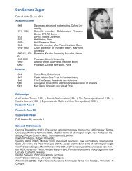
String theory is based on a remarkable generalization fromFeynman diagrams to Riemann surfaces, as illustrated by thispicture

String theory is based on a remarkable generalization fromFeynman diagrams to Riemann surfaces, as illustrated by thispicture

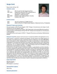
Another look, emphasizing the relation between the Schwingerparameters of a Feynman diagram and the complex modularparameters of a Riemann surface, is as follows

Another look, emphasizing the relation between the Schwingerparameters of a Feynman diagram and the complex modularparameters of a Riemann surface, is as follows

Bosonic string theory – that is string theory with Riemann surfaces– resolves the ultraviolet problems of ordinary quantum fieldtheory, but it has unavoidable infrared problems associated totachyons and also to “tadpoles” of massless particles.

There is another step which is more modest than the passage fromFeynman graphs to Riemann surfaces, but in its own way is alsoquite remarkable.

There is another step which is more modest than the passage fromFeynman graphs to Riemann surfaces, but in its own way is alsoquite remarkable. This is the generalization from Riemann surfacesto super Riemann surfaces, leading to superstring theory andspacetime supersymmetry,

There is another step which is more modest than the passage fromFeynman graphs to Riemann surfaces, but in its own way is alsoquite remarkable. This is the generalization from Riemann surfacesto super Riemann surfaces, leading to superstring theory andspacetime supersymmetry, and providing a framework to resolvethe infrared questions.

Riemann surfaces are certainly very familiar to string theorists, andsince complex manifolds of higher dimension are also important instring theory, to some extent string theorists have becomealgebraic geometers.

Riemann surfaces are certainly very familiar to string theorists, andsince complex manifolds of higher dimension are also important instring theory, to some extent string theorists have becomealgebraic geometers. But super Riemann surfaces have not becomeso well known, even among string theorists, and the subject hasnot been so well developed.

Riemann surfaces are certainly very familiar to string theorists, andsince complex manifolds of higher dimension are also important instring theory, to some extent string theorists have becomealgebraic geometers. But super Riemann surfaces have not becomeso well known, even among string theorists, and the subject hasnot been so well developed. Partly in consequence, although thekey ideas of superstring perturbation theory were well establishedin the 1980’s, some nagging details were never settled.

One reason that super Riemann surfaces are not that well known,even among physicists who actually use superstring perturbationtheory, is that in low orders, it is possible in a reasonably simpleway to eliminate the “super” structure and express everything interms of ordinary Riemann surfaces.

One reason that super Riemann surfaces are not that well known,even among physicists who actually use superstring perturbationtheory, is that in low orders, it is possible in a reasonably simpleway to eliminate the “super” structure and express everything interms of ordinary Riemann surfaces. This is usually done inpractice, following ideas introduced by Friedan, Martinec, andShenker in 1985.

One reason that super Riemann surfaces are not that well known,even among physicists who actually use superstring perturbationtheory, is that in low orders, it is possible in a reasonably simpleway to eliminate the “super” structure and express everything interms of ordinary Riemann surfaces. This is usually done inpractice, following ideas introduced by Friedan, Martinec, andShenker in 1985. However, if one tries to base a general, all genusapproach to superstring perturbation theory on reducing everythingto ordinary Riemann surfaces, then things soon become highlyunintuitive and untransparent.

The natural way to develop superstring perturbation theory is interms of super Riemann surface theory.

The natural way to develop superstring perturbation theory is interms of super Riemann surface theory. There has beensurprisingly little work along these lines, though a celebrated genus2 calculation by E. D’Hoker and D. H. Phong used this framework,and an approach to a general story was made in a series ofremarkable but little-known papers in the 1990’s by A. Belopolsky.

A super Riemann surface (with N = 1 SUSY) is a supermanifold ofdimension 1|1, but it has much more structure than that (seeRosly, A. Schwarz, and Voronov (1988) for what I will say andmuch more). There are far too many 1|1 supermanifolds.

A super Riemann surface (with N = 1 SUSY) is a supermanifold ofdimension 1|1, but it has much more structure than that (seeRosly, A. Schwarz, and Voronov (1988) for what I will say andmuch more). There are far too many 1|1 supermanifolds. Just likefor ordinary complex manifolds, any generic equation will define a1|1 supermanifold.

A super Riemann surface (with N = 1 SUSY) is a supermanifold ofdimension 1|1, but it has much more structure than that (seeRosly, A. Schwarz, and Voronov (1988) for what I will say andmuch more). There are far too many 1|1 supermanifolds. Just likefor ordinary complex manifolds, any generic equation will define a1|1 supermanifold. For example, in CP 2|1 with homogeneouscoordinates x, y, z|θ, we could define a 1|1 supermanifold byimposing more or less any equation, such aswhere α is an odd parameter.x 4 + y 4 + z 4 + αxyzθ = 0

A super Riemann surface (with N = 1 SUSY) is a supermanifold ofdimension 1|1, but it has much more structure than that (seeRosly, A. Schwarz, and Voronov (1988) for what I will say andmuch more). There are far too many 1|1 supermanifolds. Just likefor ordinary complex manifolds, any generic equation will define a1|1 supermanifold. For example, in CP 2|1 with homogeneouscoordinates x, y, z|θ, we could define a 1|1 supermanifold byimposing more or less any equation, such asx 4 + y 4 + z 4 + αxyzθ = 0where α is an odd parameter. But it is unlikely that thatsupermanifold can be given the structure of a super Riemannsurface.

One way to define a super Riemann surface is that it is a 1|1supermanifold Σ endowed with an “everywhere nonintegrabledistribution of rank 0|1.”

One way to define a super Riemann surface is that it is a 1|1supermanifold Σ endowed with an “everywhere nonintegrabledistribution of rank 0|1.” This is an odd (or fermionic) linesub-bundle D ⊂ T Σ (where T Σ is the tangent bundle of Σ, whoserank is 1|1) such that if D is a local nonzero section of D, thenD 2 = {D, D}/2 is everywhere linearly independent of D andtherefore generates the quotient T Σ/D.

One way to define a super Riemann surface is that it is a 1|1supermanifold Σ endowed with an “everywhere nonintegrabledistribution of rank 0|1.” This is an odd (or fermionic) linesub-bundle D ⊂ T Σ (where T Σ is the tangent bundle of Σ, whoserank is 1|1) such that if D is a local nonzero section of D, thenD 2 = {D, D}/2 is everywhere linearly independent of D andtherefore generates the quotient T Σ/D. In other words, there isan exact sequence0 → D → T Σ → D 2 → 0.

If so it is always possible to pick local coordinates z, θ such that Dhas a sectionD = ∂ ∂θ + θ ∂ ∂z .

If so it is always possible to pick local coordinates z, θ such that Dhas a sectionD = ∂ ∂θ + θ ∂ ∂z .Such coordinates are called superconformal coordinates.

If so it is always possible to pick local coordinates z, θ such that Dhas a sectionD = ∂ ∂θ + θ ∂ ∂z .Such coordinates are called superconformal coordinates. Thesuperconformal generators (i.e., the vector fields that preserve D)are then locally of the form f (z)(∂ θ − θ∂ z ) and−(f (z)(∂ θ − θ∂ z )) 2 = g ∂ ∂z + g ′which are familiar formulas.2 θ ∂ ∂θ , g = f 2 ,

Super Riemann surfaces are much more similar to ordinaryRiemann surfaces than a generic 1|1 supermanifold would be.

Super Riemann surfaces are much more similar to ordinaryRiemann surfaces than a generic 1|1 supermanifold would be. Letme give an elementary example.

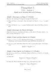
Super Riemann surfaces are much more similar to ordinaryRiemann surfaces than a generic 1|1 supermanifold would be. Letme give an elementary example. On an ordinary Riemann surface,we can remove a point and conformally map its puncturedneighborhood to a cylinder, giving the operator-statecorrespondence.

Super Riemann surfaces are much more similar to ordinaryRiemann surfaces than a generic 1|1 supermanifold would be. Letme give an elementary example. On an ordinary Riemann surface,we can remove a point and conformally map its puncturedneighborhood to a cylinder, giving the operator-statecorrespondence.

On a 1|1 supermanifold, what one needs to project to infinity hereis a divisor, of complex codimension 1|0, not a point, of complexcodimension 1|1.

On a 1|1 supermanifold, what one needs to project to infinity hereis a divisor, of complex codimension 1|0, not a point, of complexcodimension 1|1. So on a 1|1 supermanifold, one could not expectan operator-state correspondence of the usual form for operatorssupported at a point.

On a 1|1 supermanifold, what one needs to project to infinity hereis a divisor, of complex codimension 1|0, not a point, of complexcodimension 1|1. So on a 1|1 supermanifold, one could not expectan operator-state correspondence of the usual form for operatorssupported at a point. However, on a super Riemann surface, itdoes work, since on a super Riemann surface any point p doesdetermine a divisor E p , namely the divisor containing p whosetangent space coincides with the fiber of D at p.

On a 1|1 supermanifold, what one needs to project to infinity hereis a divisor, of complex codimension 1|0, not a point, of complexcodimension 1|1. So on a 1|1 supermanifold, one could not expectan operator-state correspondence of the usual form for operatorssupported at a point. However, on a super Riemann surface, itdoes work, since on a super Riemann surface any point p doesdetermine a divisor E p , namely the divisor containing p whosetangent space coincides with the fiber of D at p. Giving thetangent space to a divisor E p at a point p would not completely fixE p in ordinary algebraic geometry, but it works here because we arediscussing a very little divisor, of dimension 0|1.

Another way to say it is that the divisor E p is defined by the idealof functions that obeyfor any section D of D.f (p) = Df (p) = 0

Another way to say it is that the divisor E p is defined by the idealof functions that obeyf (p) = Df (p) = 0for any section D of D. This ideal is principal, so it defines adivisor. For instance, in local coordinates z|θ, if p is the pointz = θ = 0, then the ideal in question is generated by z; note thatDθ ≠ 0 at p.

Another way to say it is that the divisor E p is defined by the idealof functions that obeyf (p) = Df (p) = 0for any section D of D. This ideal is principal, so it defines adivisor. For instance, in local coordinates z|θ, if p is the pointz = θ = 0, then the ideal in question is generated by z; note thatDθ ≠ 0 at p. Concretely, what I have told you is that on a superRiemann surface, the point z = θ = 0 canonically determines thedivisor z = 0.

Another way to say it is that the divisor E p is defined by the idealof functions that obeyf (p) = Df (p) = 0for any section D of D. This ideal is principal, so it defines adivisor. For instance, in local coordinates z|θ, if p is the pointz = θ = 0, then the ideal in question is generated by z; note thatDθ ≠ 0 at p. Concretely, what I have told you is that on a superRiemann surface, the point z = θ = 0 canonically determines thedivisor z = 0. The divisor E p , not just the point p, is projected toinfinity when we make the operator-state correspondence for anoperator that is supported at a point on a super Riemann surfaceΣ.

Accordingly, on a super Riemann surface, a point can sometimesbehave like a divisor, just as on an ordinary Riemann surface andunlike the case of a generic 1|1 supermanifold.

In fact, in superstring theory, there are two kinds of vertexoperator. A Neveu-Schwarz vertex operator is a field Φ(z, θ) thatis inserted at a point z, θ ∈ Σ and thus what I have said appliesdirectly to such vertex operators.

In fact, in superstring theory, there are two kinds of vertexoperator. A Neveu-Schwarz vertex operator is a field Φ(z, θ) thatis inserted at a point z, θ ∈ Σ and thus what I have said appliesdirectly to such vertex operators. But a Ramond vertex operatorlives at a singularity in the superconformal structure.

In fact, in superstring theory, there are two kinds of vertexoperator. A Neveu-Schwarz vertex operator is a field Φ(z, θ) thatis inserted at a point z, θ ∈ Σ and thus what I have said appliesdirectly to such vertex operators. But a Ramond vertex operatorlives at a singularity in the superconformal structure. Here we stillendow Σ with a subbundle D ⊂ T Σ, but now a generating sectionD of D has the property that D 2 vanishes on a divisor in Σ; aRamond vertex operator is inserted at such a divisor.

In fact, in superstring theory, there are two kinds of vertexoperator. A Neveu-Schwarz vertex operator is a field Φ(z, θ) thatis inserted at a point z, θ ∈ Σ and thus what I have said appliesdirectly to such vertex operators. But a Ramond vertex operatorlives at a singularity in the superconformal structure. Here we stillendow Σ with a subbundle D ⊂ T Σ, but now a generating sectionD of D has the property that D 2 vanishes on a divisor in Σ; aRamond vertex operator is inserted at such a divisor. The localstructure isD = ∂ ∂θ + zθ ∂ ∂zso D 2 = z∂/∂z and vanishes on the divisor z = 0.

Friedan, Martinec, and Shenker in 1985 explained what kind ofvertex operators are inserted at such superconformal singularities –they are often called spin fields – and how to compute theiroperator product expansions.

Friedan, Martinec, and Shenker in 1985 explained what kind ofvertex operators are inserted at such superconformal singularities –they are often called spin fields – and how to compute theiroperator product expansions. In particular, the operators thatgenerate spacetime supersymmetry are of this kind, so their workmade it possible to see spacetime supersymmetry in a covariantway in superstring theory.

Thus Ramond vertex operators are directly associated to divisors –though this is not usually stated – while NS vertex operators canbe associated to divisors via the map from points to divisors on asuper Riemann surface.

To understand superstring perturbation theory requires a littlemore sophistication with supermanifolds and integration over themthan one needs for typical problems in supersymmetry andsupergravity.

To understand superstring perturbation theory requires a littlemore sophistication with supermanifolds and integration over themthan one needs for typical problems in supersymmetry andsupergravity. That is probably the main reason for any unclaritythat surrounds it.

Some low order cases are deceptively simple and really don’t give agood idea of a general algorithm for superstring perturbationtheory.

Some low order cases are deceptively simple and really don’t give agood idea of a general algorithm for superstring perturbationtheory. For example, in genus g = 1, the dilaton tadpole vanishesin R 10 by summing over spin structures, but the fact that thismakes sense depends upon the fact that in g = 1 (with nopunctures) there are no fermionic moduli.

Some low order cases are deceptively simple and really don’t give agood idea of a general algorithm for superstring perturbationtheory. For example, in genus g = 1, the dilaton tadpole vanishesin R 10 by summing over spin structures, but the fact that thismakes sense depends upon the fact that in g = 1 (with nopunctures) there are no fermionic moduli. As soon as there are oddmoduli, there is no meaningful notion of two super Riemannsurfaces being the same but with different spin structures.

Some low order cases are deceptively simple and really don’t give agood idea of a general algorithm for superstring perturbationtheory. For example, in genus g = 1, the dilaton tadpole vanishesin R 10 by summing over spin structures, but the fact that thismakes sense depends upon the fact that in g = 1 (with nopunctures) there are no fermionic moduli. As soon as there are oddmoduli, there is no meaningful notion of two super Riemannsurfaces being the same but with different spin structures. Inparticular, in genus g > 1, there is no meaningful operation ofsumming over spin structures without integrating oversupermoduli.

Some low order cases are deceptively simple and really don’t give agood idea of a general algorithm for superstring perturbationtheory. For example, in genus g = 1, the dilaton tadpole vanishesin R 10 by summing over spin structures, but the fact that thismakes sense depends upon the fact that in g = 1 (with nopunctures) there are no fermionic moduli. As soon as there are oddmoduli, there is no meaningful notion of two super Riemannsurfaces being the same but with different spin structures. Inparticular, in genus g > 1, there is no meaningful operation ofsumming over spin structures without integrating oversupermoduli. In genus g = 2, D’Hoker and Phong found aneffective and very beautiful way to integrate over fermionic modulifirst (after which the sum over spin structures makes sense andcould be used to show the vanishing of the dilaton tadpole) andthen integrate over bosonic moduli.

Some low order cases are deceptively simple and really don’t give agood idea of a general algorithm for superstring perturbationtheory. For example, in genus g = 1, the dilaton tadpole vanishesin R 10 by summing over spin structures, but the fact that thismakes sense depends upon the fact that in g = 1 (with nopunctures) there are no fermionic moduli. As soon as there are oddmoduli, there is no meaningful notion of two super Riemannsurfaces being the same but with different spin structures. Inparticular, in genus g > 1, there is no meaningful operation ofsumming over spin structures without integrating oversupermoduli. In genus g = 2, D’Hoker and Phong found aneffective and very beautiful way to integrate over fermionic modulifirst (after which the sum over spin structures makes sense andcould be used to show the vanishing of the dilaton tadpole) andthen integrate over bosonic moduli. This calculation is currentlythe gold standard, but actually for generic g their procedure has noanalog and the only natural operation is the combined integral overall bosonic and fermionic moduli. (A precise statement along theselines is the topic of the next lecture by Donagi.)

Instead of talking more about what doesn’t work in general, let usdiscuss what does work.

Instead of talking more about what doesn’t work in general, let usdiscuss what does work. First of all, there is a natural measure onsupermoduli space, which I will call ˜Mg,n . This was constructed inthe 1980’s via conformal field theory (in varied approaches byMoore, Nelson, and Polchinski; E. & H. Verlinde; and D’Hoker andPhong) by adapting the analogous formulas for the bosonic string.

Instead of talking more about what doesn’t work in general, let usdiscuss what does work. First of all, there is a natural measure onsupermoduli space, which I will call ˜Mg,n . This was constructed inthe 1980’s via conformal field theory (in varied approaches byMoore, Nelson, and Polchinski; E. & H. Verlinde; and D’Hoker andPhong) by adapting the analogous formulas for the bosonic string.Also, though less well known, there is for the important case ofstrings in R 10 a slightly abstract but very elegant – and completelyrigorous mathematically – construction of the measure by Rosly,Schwarz and Voronov (1988) via algebraic geometry.

Another key point is that integration of a smooth measure on acompact supermanifold is a well-defined operation just as on anordinary manifold.

Another key point is that integration of a smooth measure on acompact supermanifold is a well-defined operation just as on anordinary manifold. I will say a little more about that later.

Supermoduli space is not compact – or if we take itsDeligne-Mumford compactification, then the measure we want tointegrate has singularities – because the infrared singularities thatare crucial to the physical interpretation of string theory arise fromthe behavior of the measure at infinity

Although supermoduli space is very subtle, if one asks precisely thequestions whose answers one needs, those particular questions tendto have simple answers.

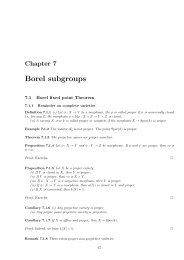
For example, the description of the moduli space near a node ordouble point is nearly as simple as for a bosonic Riemann surface.

For example, the description of the moduli space near a node ordouble point is nearly as simple as for a bosonic Riemann surface.In the bosonic case, the gluing of a surface with local parameter xto one with local parameter y is byxy = q.

For example, the description of the moduli space near a node ordouble point is nearly as simple as for a bosonic Riemann surface.In the bosonic case, the gluing of a surface with local parameter xto one with local parameter y is byxy = q.For the super case, we have to decide whether the string statepropagating through the double point is in the NS or Ramondsector.

For example, the description of the moduli space near a node ordouble point is nearly as simple as for a bosonic Riemann surface.In the bosonic case, the gluing of a surface with local parameter xto one with local parameter y is byxy = q.For the super case, we have to decide whether the string statepropagating through the double point is in the NS or Ramondsector. But either way, there is a formula almost as simple as thebosonic one.

For instance, in the NS sector, the gluing of local superconformalparameters x, θ to y, ψ is byxy = ε 2 ,yθ = εψ, xψ = εθ.

For instance, in the NS sector, the gluing of local superconformalparameters x, θ to y, ψ is byxy = ε 2 ,yθ = εψ, xψ = εθ.Importantly, the gluing depends in both cases on only one bosonicparameter ε and no fermionic ones, just as for bosonic Riemannsurfaces.

For instance, in the NS sector, the gluing of local superconformalparameters x, θ to y, ψ is byxy = ε 2 ,yθ = εψ, xψ = εθ.Importantly, the gluing depends in both cases on only one bosonicparameter ε and no fermionic ones, just as for bosonic Riemannsurfaces. The locus ε = 0 in ˜M g,n is a product of spaces of thesame type ˜M g1 ,n 1 +1 × ˜M g2 ,n 2 +1 with g 1 + g 2 = g, n 1 + n 2 = n,just as for bosonic Riemann surfaces.

For instance, in the NS sector, the gluing of local superconformalparameters x, θ to y, ψ is byxy = ε 2 ,yθ = εψ, xψ = εθ.Importantly, the gluing depends in both cases on only one bosonicparameter ε and no fermionic ones, just as for bosonic Riemannsurfaces. The locus ε = 0 in ˜M g,n is a product of spaces of thesame type ˜M g1 ,n 1 +1 × ˜M g2 ,n 2 +1 with g 1 + g 2 = g, n 1 + n 2 = n,just as for bosonic Riemann surfaces. This factorization is a step inproving a physically sensible behavior of singularities associated toon-shell string states.

For another example, although a sum over spin structures(independent of the integration over supermoduli) does not makesense in general, a very small piece of it makes sense when a nodedevelopsand this leads to theGSO projection on the physical states that propagate through thenode.

Actually, the GSO projection is almost a consequence of the gluingformulas that I presented a moment ago.

Actually, the GSO projection is almost a consequence of the gluingformulas that I presented a moment ago. You may have noticedthat the classical gluing parameter q becomes ε 2 for superRiemann surfaces. For given q, there are two choices of ε, and thesum over these two choices gives the GSO projection.

Let me mention at least a few of the important structures inbosonic string theory that one has to generalize to super Riemannsurfaces in order to have a good foundation for superstringperturbation theory. If X is an observable – for example a productX = V 1 V 2 . . . V n of vertex operators – then there is an associateddifferential form F X on M g,n .

Let me mention at least a few of the important structures inbosonic string theory that one has to generalize to super Riemannsurfaces in order to have a good foundation for superstringperturbation theory. If X is an observable – for example a productX = V 1 V 2 . . . V n of vertex operators – then there is an associateddifferential form F X on M g,n . Anomalous ghost number symmetrydetermines the degree of F X in terms of the ghost number of X .(For instance, if X is a product of physical state vertex operators,then F X is a form of top degree.)

The association X → F X is also compatible with BRST symmetryin the sense that (with Q the BRST operator)F QX + dF X = 0.

This is the basis of the proof of gauge-invariance. Usually oneconsiders a product of physical state vertex operators V 1 , . . . , V n ,all of them annihilated by Q. One makes a gauge transformationV 1 → V 1 + {Q, W 1 }, for some W 1 . This shifts the scatteringamplitude by∫∫F V1 V 2 ...V n→ (F V1 V 2 ...V n+ F QW1 V 2 ...V n) .M g,n M g,n

This is the basis of the proof of gauge-invariance. Usually oneconsiders a product of physical state vertex operators V 1 , . . . , V n ,all of them annihilated by Q. One makes a gauge transformationV 1 → V 1 + {Q, W 1 }, for some W 1 . This shifts the scatteringamplitude by∫∫F V1 V 2 ...V n→ (F V1 V 2 ...V n+ F QW1 V 2 ...V n) .M g,n M g,nThe extra term that should vanish to establish gauge invariance isthus ∫F QW1 V 2 ...V n= −M g,n∫dF W1 V 2 ...V nM g,nwhere I used the compatibility of X → F X with BRST symmetry.

This is the basis of the proof of gauge-invariance. Usually oneconsiders a product of physical state vertex operators V 1 , . . . , V n ,all of them annihilated by Q. One makes a gauge transformationV 1 → V 1 + {Q, W 1 }, for some W 1 . This shifts the scatteringamplitude by∫∫F V1 V 2 ...V n→ (F V1 V 2 ...V n+ F QW1 V 2 ...V n) .M g,n M g,nThe extra term that should vanish to establish gauge invariance isthus ∫F QW1 V 2 ...V n= −M g,n∫dF W1 V 2 ...V nM g,nwhere I used the compatibility of X → F X with BRST symmetry.Finally we have Stokes’s theorem∫∫dF W1 V 2 ...V n= − F W1 V 2 ...V n.M g,n ∂M g,nThus gauge-invariance finally depends only on the behavior of theform F W1 V 2 ...V nin the infrared region, that is at infinity in M g,n .

So this is the package that one needs to carry over to superRiemann surfaces in order to have a proper foundation forsuperstring perturbation theory. One needs an associationX → F X of observables to forms on moduli space, which mapsghost number to degree and maps the BRST operator Q to theexterior derivative d. And one needs Stokes’s theorem so that onecan integrate by parts.

So this is the package that one needs to carry over to superRiemann surfaces in order to have a proper foundation forsuperstring perturbation theory. One needs an associationX → F X of observables to forms on moduli space, which mapsghost number to degree and maps the BRST operator Q to theexterior derivative d. And one needs Stokes’s theorem so that onecan integrate by parts. It turns out that when one works out whatthese things mean in supergeometry, one meets another structure,picture number, which was part of the framework of Friedan,Martinec, and Shenker (and then was interpreted moregeometrically by E. and H. Verlinde and then by Belopolsky).

Once one has this package (along with the foundational results ofthe 1980’s such as the construction of the fermion vertex operator)one has a good framework to understand spacetimesupersymmetry, which is really a special case of gauge-invariance.

Once one has this package (along with the foundational results ofthe 1980’s such as the construction of the fermion vertex operator)one has a good framework to understand spacetimesupersymmetry, which is really a special case of gauge-invariance.And spacetime supersymmetry – along with generalities of theDeligne-Mumford compactification – gives a good tool to clarifythe unresolved details about the infrared behavior of superstringperturbation theory.

It is not really possible to explain everything in one lecture, soperhaps I will focus on explaining the notion of forms on asupermanifold, picture number, and Stokes’s theorem.

It is not really possible to explain everything in one lecture, soperhaps I will focus on explaining the notion of forms on asupermanifold, picture number, and Stokes’s theorem. Supposethat M is a bosonic manifold with local coordinates x 1 , . . . , x n .

It is not really possible to explain everything in one lecture, soperhaps I will focus on explaining the notion of forms on asupermanifold, picture number, and Stokes’s theorem. Supposethat M is a bosonic manifold with local coordinates x 1 , . . . , x n .We let ΠTM be the cotangent bundle with “parity” (or statistics)reversed on the fibers, so local coordinates on ΠTM are x 1 , . . . , x nand corresponding fermionic variables that we will calldx 1 , . . . , dx n .

A function on ΠTM can be expanded in powers of the dx’sf (x 1 , . . . , x n |dx 1 . . . dx n ) = f 0 (x 1 . . . x n ) + ∑ idx i f 1,i (x 1 , . . . , x n )+ ∑ dx i dx j f 2,ij (x 1 , . . . , x n ) + . . . .i

A function on ΠTM can be expanded in powers of the dx’sf (x 1 , . . . , x n |dx 1 . . . dx n ) = f 0 (x 1 . . . x n ) + ∑ idx i f 1,i (x 1 , . . . , x n )+ ∑ i

One can think of integration of forms as the Berezin integral onΠTM.

One can think of integration of forms as the Berezin integral onΠTM. Recall the Berezin integral: for an odd variable θ,∫Dθ 1 = 0,∫Dθ θ = 1.

One can think of integration of forms as the Berezin integral onΠTM. Recall the Berezin integral: for an odd variable θ,∫Dθ 1 = 0,∫Dθ θ = 1. There is a natural measure D(x, dx) onΠTM (for example, in a change of variables x → λx, dx → λdx,D(x, dx) is invariant because the fermion measure transformsoppositely to the boson measure).

One can think of integration of forms as the Berezin integral onΠTM. Recall the Berezin integral: for an odd variable θ,∫Dθ 1 = 0,∫Dθ θ = 1. There is a natural measure D(x, dx) onΠTM (for example, in a change of variables x → λx, dx → λdx,D(x, dx) is invariant because the fermion measure transformsoppositely to the boson measure). We just integrate aninhomogeneous differential form with the natural measure measure∫D(x, dx).

So for example iff (x, dx) = · · · + dx 1 dx 2 . . . dx n f (n) (x 1 , . . . , x n ),where I have only written the n-form part of f , then the Berezinintegral over the dx i picks out the n-form part of f

So for example iff (x, dx) = · · · + dx 1 dx 2 . . . dx n f (n) (x 1 , . . . , x n ),where I have only written the n-form part of f , then the Berezinintegral over the dx i picks out the n-form part of f and as a resultthe integral in this sense∫D(x, dx) f (x, dx)ΠTMis the integral of the differential form f (n) in the usual way.

So for example iff (x, dx) = · · · + dx 1 dx 2 . . . dx n f (n) (x 1 , . . . , x n ),where I have only written the n-form part of f , then the Berezinintegral over the dx i picks out the n-form part of f and as a resultthe integral in this sense∫D(x, dx) f (x, dx)ΠTMis the integral of the differential form f (n) in the usual way. Asnotation, we write∫∫f (x, dx) = D(x, dx) f (x, dx).MΠTM

On ΠTM, there is a vector field of degree 1d =n∑dx i ∂∂x ii=1and Stokes’s theorem says that∫ ∫dg =M∂Mg.

Up to a certain point, we can imitate this for supermanifolds. Tosee the essential point that is new, consider a purely fermionicsupermanifold M = R 0|n with odd coordinates θ 1 . . . θ m .

Up to a certain point, we can imitate this for supermanifolds. Tosee the essential point that is new, consider a purely fermionicsupermanifold M = R 0|n with odd coordinates θ 1 . . . θ m . So nowthe fiber coordinates of ΠTM are even variables that we calldθ 1 , . . . dθ m .

Up to a certain point, we can imitate this for supermanifolds. Tosee the essential point that is new, consider a purely fermionicsupermanifold M = R 0|n with odd coordinates θ 1 . . . θ m . So nowthe fiber coordinates of ΠTM are even variables that we calldθ 1 , . . . dθ m . It is still true that there is a natural Berezin measureD(θ, dθ) since the Berezinian of the tangent bundle of ΠTMcoming from any reparametrization of M is 1, due to cancellationbetween θ and dθ. So one might expect to integrate a function onΠTM as before.

However, there is a key difference from the bosonic case: there aredifferent classes of functions on ΠTM. For an ordinary manifoldM, the fiber coordinates dx i were fermionic variables, so anyfunction on ΠTM was a polynomial along the fibers. We did nothave to choose a class of functions.

However, there is a key difference from the bosonic case: there aredifferent classes of functions on ΠTM. For an ordinary manifoldM, the fiber coordinates dx i were fermionic variables, so anyfunction on ΠTM was a polynomial along the fibers. We did nothave to choose a class of functions. For M = R 0,n , the fibercoordinates are even and there definitely are different classes offunctions on ΠTM.

For example, we can consider functions on ΠTM that arepolynomials in the dθ’s. These functions are called differentialforms.

For example, we can consider functions on ΠTM that arepolynomials in the dθ’s. These functions are called differentialforms. They are closed under many natural operations, but theycannot be integrated, because obviously, with dθ being an ordinaryeven variable, an integral∫D(θ, dθ) f (θ, dθ)diverges if f (θ, dθ) is a polynomial in dθ.

By contrast, we can integrate forms that have distributionalsupport at dθ = 0.

By contrast, we can integrate forms that have distributionalsupport at dθ = 0. Let us consider the case of just one θ and dθ.By distributional support I mean a form that is proportional toδ(dθ) or a derivative of this of finite order:g(θ, dθ) = g −1 (θ)δ(dθ) + g −2 (θ)δ ′ (dθ) + g −3 (θ)δ (2) (dθ) + . . . .

By contrast, we can integrate forms that have distributionalsupport at dθ = 0. Let us consider the case of just one θ and dθ.By distributional support I mean a form that is proportional toδ(dθ) or a derivative of this of finite order:g(θ, dθ) = g −1 (θ)δ(dθ) + g −2 (θ)δ ′ (dθ) + g −3 (θ)δ (2) (dθ) + . . . .We call such a g(θ, dθ) an integral form (delta function supportalong M ⊂ ΠTM).

By contrast, we can integrate forms that have distributionalsupport at dθ = 0. Let us consider the case of just one θ and dθ.By distributional support I mean a form that is proportional toδ(dθ) or a derivative of this of finite order:g(θ, dθ) = g −1 (θ)δ(dθ) + g −2 (θ)δ ′ (dθ) + g −3 (θ)δ (2) (dθ) + . . . .We call such a g(θ, dθ) an integral form (delta function supportalong M ⊂ ΠTM). The subscripts I have chosen label the“degree” of an integral form, where by degree I mean the scalingunder dθ → λdθ.

By contrast, we can integrate forms that have distributionalsupport at dθ = 0. Let us consider the case of just one θ and dθ.By distributional support I mean a form that is proportional toδ(dθ) or a derivative of this of finite order:g(θ, dθ) = g −1 (θ)δ(dθ) + g −2 (θ)δ ′ (dθ) + g −3 (θ)δ (2) (dθ) + . . . .We call such a g(θ, dθ) an integral form (delta function supportalong M ⊂ ΠTM). The subscripts I have chosen label the“degree” of an integral form, where by degree I mean the scalingunder dθ → λdθ. Note that for integral forms there is a form oftop degree (namely degree −1 in the case of a single odd variable,since the function δ(dθ) has degree −1), but no form of bottomdegree (δ (n) (dθ) has degree −1 − n for any n).

Integral forms can be integrated∫∫g(θ, dθ) = D(θ, dθ)g(θ, dθ).M

Integral forms can be integrated∫∫g(θ, dθ) = D(θ, dθ)g(θ, dθ).MConcretely the integral over dθ picks out the top form g −1 and so∫∫g(θ, dθ) = D(θ) g −1 (θ)Mwhere the last integral is a Berezin integral.

Another natural operation is the exterior derivative, again derivedfrom a vector field on ΠTM of degree 1, nowd =n∑dθ i ∂∂θ i .i=1

Another natural operation is the exterior derivative, again derivedfrom a vector field on ΠTM of degree 1, nowd =n∑dθ i ∂∂θ i .i=1For the case of a purely fermionic supermanifold R 0|n , Stokes’stheorem says that for any integral form g,∫dg = 0.M

For instance, ifg(θ, dθ) = g −1 (θ)δ(dθ) + g −2 (θ)δ ′ (dθ) + g −3 (θ)δ (2) (dθ) + . . . ,thendg = − ∂ ∂θ g −2(θ)δ(dθ) + . . .where I use d = dθ∂ θ , and dθδ ′ (dθ) = −δ(dθ),

For instance, ifg(θ, dθ) = g −1 (θ)δ(dθ) + g −2 (θ)δ ′ (dθ) + g −3 (θ)δ (2) (dθ) + . . . ,thendg = − ∂ ∂θ g −2(θ)δ(dθ) + . . .where I use d = dθ∂ θ , and dθδ ′ (dθ) = −δ(dθ), so∫ ∫dg = − D(θ) ∂ ∂θ g −2(θ) = 0.M

For instance, ifg(θ, dθ) = g −1 (θ)δ(dθ) + g −2 (θ)δ ′ (dθ) + g −3 (θ)δ (2) (dθ) + . . . ,thendg = − ∂ ∂θ g −2(θ)δ(dθ) + . . .where I use d = dθ∂ θ , and dθδ ′ (dθ) = −δ(dθ), so∫ ∫dg = − D(θ) ∂ ∂θ g −2(θ) = 0.MThe general supermanifold version of Stokes’s theorem is more orless a combination of this with the ordinary bosonic Stokes’stheorem.

I have described differential forms (polynomial dependence on alldθ’s) and integral forms (delta function dependence on all dθ’s.More generally, one considers other classes of forms that are closedunder various natural operations (such as scaling of dθ,multiplication by dθ, and differentiation ∂/∂(dθ)).

I have described differential forms (polynomial dependence on alldθ’s) and integral forms (delta function dependence on all dθ’s.More generally, one considers other classes of forms that are closedunder various natural operations (such as scaling of dθ,multiplication by dθ, and differentiation ∂/∂(dθ)). A form is saidto have picture number −k if it has delta function localization withrespect to k dθ’s. (The sign comes from the convention used byFriedan, Martinec, and Shenker.)

I have described differential forms (polynomial dependence on alldθ’s) and integral forms (delta function dependence on all dθ’s.More generally, one considers other classes of forms that are closedunder various natural operations (such as scaling of dθ,multiplication by dθ, and differentiation ∂/∂(dθ)). A form is saidto have picture number −k if it has delta function localization withrespect to k dθ’s. (The sign comes from the convention used byFriedan, Martinec, and Shenker.) In general, if one wants to beable to integrate a form over a submanifold of M of dimension p|q,it should have degree p − q and picture number −q.

Obviously we can’t go into a full explanation today, but it turnsout that superstring perturbation theory is nicely compatible withthis formalism and this gives a natural framework to understandgauge-invariance, spacetime supersymmetry, and tadpolecancellation.

The traditional alternative is to look for a map from ˜M g,n toM g,n (a map that is the identity when restricted toM g,n ⊂ ˜M g,n ) and try to formulate everything in terms ofmeasures on M g,n .

The traditional alternative is to look for a map from ˜M g,n toM g,n (a map that is the identity when restricted toM g,n ⊂ ˜M g,n ) and try to formulate everything in terms ofmeasures on M g,n . If there is a holomorphic map of this kind, it iscalled a splitting of supermoduli space.

The traditional alternative is to look for a map from ˜M g,n toM g,n (a map that is the identity when restricted toM g,n ⊂ ˜M g,n ) and try to formulate everything in terms ofmeasures on M g,n . If there is a holomorphic map of this kind, it iscalled a splitting of supermoduli space. Practical calculations havebeen based on the existence of such splittings at low orders. (Thisis not always made explicit.)

The traditional alternative is to look for a map from ˜M g,n toM g,n (a map that is the identity when restricted toM g,n ⊂ ˜M g,n ) and try to formulate everything in terms ofmeasures on M g,n . If there is a holomorphic map of this kind, it iscalled a splitting of supermoduli space. Practical calculations havebeen based on the existence of such splittings at low orders. (Thisis not always made explicit.) When there is a holomorphicsplitting, it can be used to push down the possibly natural formulason ˜M g,n to formulas on M g,n that still at least have reasonableproperties of holomorphy.

The traditional alternative is to look for a map from ˜M g,n toM g,n (a map that is the identity when restricted toM g,n ⊂ ˜M g,n ) and try to formulate everything in terms ofmeasures on M g,n . If there is a holomorphic map of this kind, it iscalled a splitting of supermoduli space. Practical calculations havebeen based on the existence of such splittings at low orders. (Thisis not always made explicit.) When there is a holomorphicsplitting, it can be used to push down the possibly natural formulason ˜M g,n to formulas on M g,n that still at least have reasonableproperties of holomorphy. This can be especially useful if M g,n iswell-understood, which tends to be so for small g.

The point of the next talk by Donagi will be to show that such asplitting does not exist in general.

The point of the next talk by Donagi will be to show that such asplitting does not exist in general. I feel that it was reasonable toexpect this result for a variety of reasons.

The point of the next talk by Donagi will be to show that such asplitting does not exist in general. I feel that it was reasonable toexpect this result for a variety of reasons. The existence of asplitting is not necessary for superstring perturbation theory towork, and I believe that the experience with super Riemannsurfaces is that they have only those simplifying features that areneeded for superstring perturbation theory.

The point of the next talk by Donagi will be to show that such asplitting does not exist in general. I feel that it was reasonable toexpect this result for a variety of reasons. The existence of asplitting is not necessary for superstring perturbation theory towork, and I believe that the experience with super Riemannsurfaces is that they have only those simplifying features that areneeded for superstring perturbation theory. If one looks carefully atthe splittings that do exist in low genus, one finds that they behavebadly at infinity; this is actually the worst they could do in lowgenus (where the uncompactified moduli spaces are affine andhence inevitably split) and suggests that as soon as possible, themoduli spaces will be nonsplit.

The point of the next talk by Donagi will be to show that such asplitting does not exist in general. I feel that it was reasonable toexpect this result for a variety of reasons. The existence of asplitting is not necessary for superstring perturbation theory towork, and I believe that the experience with super Riemannsurfaces is that they have only those simplifying features that areneeded for superstring perturbation theory. If one looks carefully atthe splittings that do exist in low genus, one finds that they behavebadly at infinity; this is actually the worst they could do in lowgenus (where the uncompactified moduli spaces are affine andhence inevitably split) and suggests that as soon as possible, themoduli spaces will be nonsplit. Finally, even when a splitting exists,it does not make spacetime supersymmetry visible, suggesting thatone should be looking for a different approach.