Image Deformation Using Moving Least Squares - TAMU Computer ...

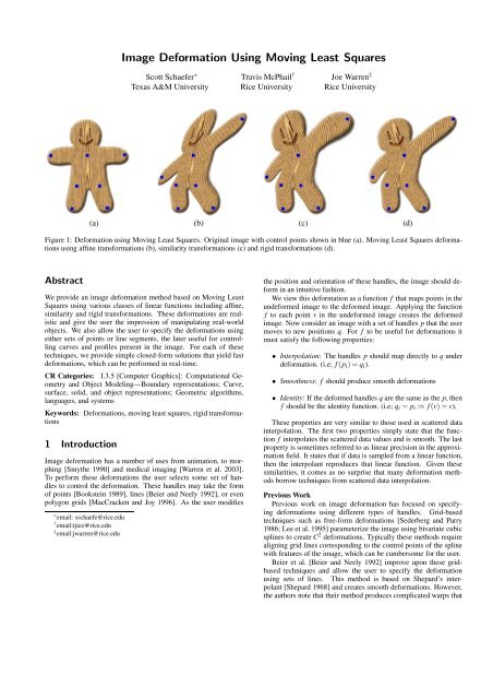
Image Deformation Using Moving Least SquaresScott Schaefer ∗Texas A&M UniversityTravis McPhail †Rice UniversityJoe Warren ‡Rice University(a) (b) (c) (d)Figure 1: Deformation using Moving Least Squares. Original image with control points shown in blue (a). Moving Least Squares deformationsusing affine transformations (b), similarity transformations (c) and rigid transformations (d).AbstractWe provide an image deformation method based on Moving LeastSquares using various classes of linear functions including affine,similarity and rigid transformations. These deformations are realisticand give the user the impression of manipulating real-worldobjects. We also allow the user to specify the deformations usingeither sets of points or line segments, the later useful for controllingcurves and profiles present in the image. For each of thesetechniques, we provide simple closed-form solutions that yield fastdeformations, which can be performed in real-time.CR Categories: I.3.5 [Computer Graphics]: Computational Geometryand Object Modeling—Boundary representations; Curve,surface, solid, and object representations; Geometric algorithms,languages, and systemsKeywords: Deformations, moving least squares, rigid transformations1 IntroductionImage deformation has a number of uses from animation, to morphing[Smythe 1990] and medical imaging [Warren et al. 2003].To perform these deformations the user selects some set of handlesto control the deformation. These handles may take the formof points [Bookstein 1989], lines [Beier and Neely 1992], or evenpolygon grids [MacCracken and Joy 1996]. As the user modifies∗ email: sschaefe@rice.edu† email:tjice@rice.edu‡ email:jwarren@rice.eduthe position and orientation of these handles, the image should deformin an intuitive fashion.We view this deformation as a function f that maps points in theundeformed image to the deformed image. Applying the functionf to each point v in the undeformed image creates the deformedimage. Now consider an image with a set of handles p that the usermoves to new positions q. For f to be useful for deformations itmust satisfy the following properties:• Interpolation: The handles p should map directly to q underdeformation. (i.e; f(p i )=q i ).• Smoothness: f should produce smooth deformations• Identity: If the deformed handles q are the same as the p, thenf should be the identity function. (i.e; q i = p i ⇒ f(v)=v).These properties are very similar to those used in scattered datainterpolation. The first two properties simply state that the functionf interpolates the scattered data values and is smooth. The lastproperty is sometimes referred to as linear precision in the approximationfield. It states that if data is sampled from a linear function,then the interpolant reproduces that linear function. Given thesesimilarities, it comes as no surprise that many deformation methodsborrow techniques from scattered data interpolation.Previous WorkPrevious work on image deformation has focused on specifyingdeformations using different types of handles. Grid-basedtechniques such as free-form deformations [Sederberg and Parry1986; Lee et al. 1995] parameterize the image using bivariate cubicsplines to create C 2 deformations. Typically these methods requirealigning grid lines corresponding to the control points of the splinewith features of the image, which can be cumbersome for the user.Beier et al. [Beier and Neely 1992] improve upon these gridbasedtechniques and allow the user to specify the deformationusing sets of lines. This method is based on Shepard’s interpolant[Shepard 1968] and creates smooth deformations. However,the authors note that their method produces complicated warps that

ContributionsIn this paper, we propose an image deformation method based onlinear Moving Least Squares. To construct deformations that minimizethe amount of local scaling and shear, we restrict the classesof transformations used in Moving Least Squares to similarity andrigid-body transformations. By using MLS, we avoid the need totriangulate the input image (as done in Igarashi et al.) and producedeformations that are globally smooth.)Next, we derive closed-form formulas for both similarity andrigid MLS deformations. These formula are simple, easy to implementand provide real-time deformations. This derivation relies ona surprising and little-known relationship between similarity transformationsand rigid transformations that minimize a common leastsquares problem. As opposed to Igarashi et al., our formulas do notrequire the use of a general linear solver.As a natural extension of our point-based method, we extend ourMLS deformation method from sets of points to sets of line segmentsand again provide closed-form expressions for the resultingdeformation method.2 Moving Least Squares DeformationFigure 2: Deformation of the test shape from figure 1 using thinplatesplines (left). The deformation is smooth but lacks realism.On the right we use the method by Igarashi et al. shown with triangulation(right). The lack of smoothness is clearly visible in thewood grain.can sometimes suffer from “ghosts”, undesirable folding in the deformation.Koba et al. [Kobayashi and Ootsubo 2003] later generalizedthis technique to surface deformations.Very few deformation methods investigate the type of transformationsthat are desirable for performing deformation. One notableexception is worked based on thin-plate splines [Bookstein 1989]that attempts to minimize the amount of bending in the deformation.Bookstein presents a deformation algorithm using the simplestdeformation handle, a point, that uses radial basis functionswith thin-plate splines. Figure 2 (left) shows an example of thedeformation created with thin-plate splines for our example in figure1. The deformation appears very similar to the affine-method infigure 1. In both cases, the test shape undergoes local non-uniformscaling and shearing, which is undesirable in many applications.Our paper builds primarily on a recent paper by Igarashi etal. [Igarashi et al. 2005] that proposes a point-based image deformationtechnique for cartoon-like images in which the resulting deformationsare as “rigid-as-possible”. Such deformation have theproperty that amount of local scaling and shearing is minimized.(The concept of rigid-as-possible transformations was itself first introducedin Alexa [Alexa et al. 2000].)To produce rigid-as-possible deformations, Igarashi et al. triangulatethe input image and solve a linear system of equations whosesize is equal to the number of vertices in the triangulation. In contrast,our method creates deformations by solving a small linearsystem (2×2) at each point in a uniform grid (see Section 4 for details).Since, we solve much smaller systems of equations, we cancreate very fast deformations of grids consisting of tens of thousandsof vertices in real-time whereas Igarashi et al. report thattheir methods slows at 300 vertices on a 1 GHz machine. Due tothe relatively small number of vertices, the deformations producedby Igarashi et al. may contain noticeable discontinuities as shownin figure 2. Figure 7 shows an equivalent deformation with ourtechnique, which appears smooth.Here we consider building image deformations based on collectionsof points with which the user controls the deformation. Let p bea set of control points and q the deformed positions of the controlpoints p. We construct a deformation function f satisfying thethree properties outlined in the introduction using Moving LeastSquares [Levin 1998]. Given a point v in the image, we solve forthe best affine transformation l v (x) that minimizes∑w i |l v (p i )−q i | 2 (1)iwhere p i and q i are row vectors and the weights w i have the formw i =1|p i − v| 2α .Because the weights w i in this least squares problem are dependenton the point of evaluation v, we call this a Moving Least Squaresminimization. Therefore, we obtain a different transformation l v (x)for each v.Now we define our deformation function f to be f(v) = l v (v).Observe that as v approaches p i , w i approaches infinity and thefunction f interpolates, (i.e; f(p i ) = q i ). Furthermore, if q i = p i ,then each l v (x) = x for all x and, therefore, f is the identity transformationf(v) = v. Finally, this deformation function f has theproperty that it is smooth everywhere (except at the control pointsp i when α ≤ 1).Now since l v (x) is an affine transformation, l v (x) consists of twoparts: a linear transformation matrix M and a translation T .l v (x)=xM+ T (2)We can actually remove the translation T from this minimizationproblem further simplifying these equations. Equation 1 isquadratic in T . Since the minimizer is where the derivatives withrespect to each of the free variables in l v (x) are zero, we can solvedirectly for T in terms of the matrix M. Taking the partial derivativeswith respect to the free variables in T produces a linear systemof equations. Solving for T yields thatT = q ∗ − p ∗ Mwhere p ∗ and q ∗ are weighted centroids.p ∗ = ∑i w i p i∑ i w iq ∗ = ∑i w i q i∑ i w iWith this observation we can substitute T into equation 2 andrewrite l v (x) in terms of the linear matrix M.l v (x)=(x− p ∗ )M+ q ∗ (3)Based on this insight, the least squares problem of equation 1 canbe rewritten as∑w i | ˆp i M− ˆq i | 2 (4)i

where ˆp i = p i − p ∗ and ˆq i = q i − q ∗ . Notice that Moving LeastSquares is very general in that the matrix M does not have to bea fully affine transformation. In fact, this framework allows us toinvestigate different classes of transformation matrices M. In particular,we are interested in the case where M is a rigid transformation.However, we first examine the case where M is an affinetransformation as the derivation is the simplest. Next we constructdeformations with similarity transformations and show how thesesolutions can be used to find closed-form solutions to Moving LeastSquare deformations with rigid transformations.2.1 Affine DeformationsFinding an affine deformation that minimizes equation 4 is straightforwardusing the classic normal equations solution.M =(∑i) −1ˆp T i w i ˆp i ∑w j ˆp T j ˆq j.jThough this solution requires the inversion of a matrix, the matrixis a constant size (2×2) and is fast to invert. With this closed-formsolution for M we can write a simple expression for the deformationfunction f a (v).f a (v)=(v− p ∗ )(∑i) −1ˆp T i w i ˆp i ∑w j ˆp T j ˆq j+ q ∗ . (5)jApplying this deformation function to each point in the image createsa new, deformed image.While the user creates these deformations by manipulating thepoints q, the points p are fixed. Since the p do not change duringdeformation, much of equation 5 can be precomputed yielding veryfast deformations. In particular, we can rewrite equation 5 in theformf a (v)=∑A j ˆq j + q ∗ .jwhere A j is a single scalar given byA j =(v− p ∗ )( ) −1∑ ˆp T i w i ˆp i w j ˆp T j .iNotice that, given a point v, everything in A j can be precomputedyielding a simple, weighted sum. Table 1 provides timing resultsfor the examples in this paper, which shows that these deformationsmay be performed over 500 times per second in our examples.Figure 1 (b) illustrates this affine Moving Least Squares deformationapplied to our test image. Unfortunately, the deformationdoes not appear very desirable due to the stretching in the arms andtorso. These artifacts are created because affine transformations includedeformations such as non-uniform scaling and shear. To eliminatethese undesirable deformations we need to consider restrictingthe linear transformation l v (x). In particular, we modify theclass of deformations l v (x) produces by restricting the transformationmatrix M from being fully linear to similarity and rigid-bodytransformations.2.2 Similarity DeformationsWhile affine transformations include effects such as non-uniformscaling and shear, many objects in reality do not undergo even thesesimple transformations. Similarity transformations are a specialsubset of affine transformations that only include translation, rotationand uniform scaling.To alter our deformation technique to only use similarity transformations,we constrain the matrix M to have the property thatM T M = λ 2 I for some scalar λ. If M is a block matrix of the formM = ( M 1 M 2)where M 1 , M 2 are column vectors of length 2, then restricting Mto be a similarity transform requires that M1 T M 1 = M2 T M 2 = λ 2and M1 T M 2 = 0. This constraint implies that M 2 = M1⊥ where ⊥ isan operator on 2D vectors such that (x,y) ⊥ =(−y,x). Though restricted,the minimization problem from equation 4 is still quadraticin M 1 and can be rephrased as finding the column vector M 1 thatminimizes∣( ∣∣∣ ˆpi∑w i− ˆp ⊥ ii)M 1 − ˆq T i2∣ .This quadratic function has a unique minimizer, which yields theoptimal transformation matrix MM = 1 ( ) ˆpiµ s∑w i− ˆp ⊥ ( ˆq T i − ˆq ⊥Ti ) (6)iiwhereµ s = ∑w i ˆp i ˆp T i .iSimilar to the affine deformations, the user manipulates the q toproduce the deformation while the p remain fixed. Using this observationwe write the deformation function f s (v) in a form thatallows us to precompute as much information as possible. f s (v) isthenf s (v)=∑ ˆq i ( 1 A i )+q ∗iµ swhere µ s and A i depend only on the p i , v and can be precomputedand A i isA i = w i( ˆpi− ˆp ⊥ i)(v− p ∗−(v− p ∗ ) ⊥ ) T. (7)As expected, similarity MLS deformations preserves angles inthe original image better than affine MLS deformations. (Transformationsthat strictly preserve angle are called conformal transformationsand have been studied extensively in [Gu and Yau 2003].)While approximate (or exact) angle preservation is a desirable propertyin many cases, allowing local scaling can often lead to undesirabledeformations. Figure 1 (c) shows an example of applyingthe similarity Moving Least Squares deformation to our test image.The result is a much more realistic looking deformation than (b).However, this deformation scales the size of the upper arm as it isstretched. To remove this scaling, we consider building deformationsusing only rigid transformations.2.3 Rigid DeformationsRecently, several works [Alexa et al. 2000; Igarashi et al. 2005]have shown that, for realistic shapes, deformations should be asrigid as possible; that is, the space of deformations should not eveninclude uniform scaling. Traditionally researchers in deformationhave been reluctant to approach this problem directly due to thenon-linear constraint that M T M = I. However, we note that closedformsolutions to this problem are known from the Iterated ClosestPoint community [Horn 1987]. Horn shows that the optimal rigidtransformation can be found in terms of eigenvalues and eigenvectorsof a covariance matrix involving the points p i and q i . We showthat these rigid deformations are related to the similarity deformationsfrom section 2.2 via the following theorem.

Figure 3: Original image (left) and its deformation using the rigidMLS method (right). After deformation, the face is thinner and sheis smiling.Theorem 2.1 Let C be the matrix that minimizes the following similarityfunctionalminM T M=λ 2 I ∑ iw i | ˆp i M− ˆq i | 2 .If C is written in the form λR where R is a rotation matrix and λ isa scalar, the rotation matrix R minimizes the rigid functionalProof: See Appendix A.minM T M=I ∑ iw i | ˆp i M− ˆq i | 2 .This theorem is valid in arbitrary dimension, however, it is veryeasy to apply in 2D. Using this theorem, we find that the rigidtransformation is exactly the same as equation 6 except that we usea different constant µ r in the solution so that M T M = I given by√((µ r =√) 2∑w i ˆq i ˆp T i +i∑w i ˆq i ˆp ⊥Tii) 2.Unlike the similarity deformation f s (v), we cannot precompute asmuch information for the rigid deformation function f r (v). However,the deformation process can still be made very efficient. Let⃗f r (v)=∑ ˆq i A iiwhere A i is defined in equation 7, which may be precomputed. Thisvector ⃗f r (v) is a rotated and scaled version of the vector v− p ∗ . Tocompute f r (v) we normalize⃗f r , scale by the length of v− p ∗ (whichalso can be precomputed), and translate by q ∗ .f r (v)=|v− p ∗ | ⃗ f r (v)|⃗f r (v)| + q ∗. (8)This method is slower than the similarity deformation due to thenormalization; however, these deformations are still very fast asshown in table 1.Figure 1 (d) shows this rigid deform applied to the test imagein (a). As opposed to the other methods, this deformation is quiterealistic and almost feels as if the user is manipulating a real object.Figures 3 and 4 show additional examples of this rigid deformationmethod. In the figure with the Mona Lisa, we deform the image tocreate a thinner facial profile and make her smile. In the figure withthe horse, we stretch the horses legs and neck to create a giraffe.Due to the use of rigid transformations, the deformation maintainsrigidity and scale locally so that the body and head of the horseretain their relative shape.Figure 4: Original image (left) and its deformation using the rigidMLS method (right).3 Deformation with Line SegmentsSo far we have considered creating deformations with MovingLeast Squares using only sets of points to control the deformation.In applications where precise control over curves such as profiles inthe image is needed, points may be insufficient for specifying thesedeformations. One solution that allows the user to control curvesprecisely is to convert these curves to dense sets of points and applya point-based deformation [Wolberg 1998]. The disadvantageof this approach is that the computation time of the deformation isproportional to the number of control points used and creating largenumbers of control points adversely affects performance.Alternatively, we desire a generalization of these Moving LeastSquares deformations from section 2 to arbitrary curves in theplane. First, assume p i (t) is the i th control curve and q i (t) is the deformedcurve corresponding to p i (t). We generalize the quadraticfunction in equation 1 by integrating over each control curve p i (t)where we assume t ∈[0,1].where w i (t) is∫ 1∑ w i (t)|p i (t)M+ T − q i (t)| 2 (9)i 0w i (t)=|p ′ i (t)||p i (t)−v| 2αand p ′ t (t) is the derivative of p i(t). (This factor of |p ′ (t)| makes theintegrals independent of the parameterization of the curve p i (t).)Now notice that, despite the integral, equation 9 is still quadratic inT and can be solved for in terms of the matrix M.T = q ∗ − p ∗ Mwhere p ∗ and q ∗ are again weighted centroids.∫ 1p ∗ = ∑i 0 w i(t)p i (t)dt∫ 1∑∫ i 0 w i(t)dt1q ∗ = ∑i 0 w i(t)q i (t)dt∫ 1∑ i 0 w i(t)dtTherefore, we rewrite equation 9 only in terms of M aswhere(10)∫ 1∑ w i (t)| ˆp i (t)M− ˆq i (t)| 2 (11)i 0ˆp i (t) = p i (t)− p ∗ˆq i (t) = q i (t)−q ∗ .

Figure 5: Deformation of the Leaning Tower of Pisa. From left to right: original image, Affine MLS, Similarity MLS and Rigid MLSdeformations.Until now, p i (t) and q i (t) have been arbitrary curves. However,the integrals in equation 11 may be difficult to evaluate for arbitraryfunctions. Instead, we restrict these functions to be line segmentsand derive closed-form solutions for the deformations in terms ofthe end-points of these segments. Similar to section 2, we first consideraffine transformations due to its relatively simple derivationand then move to similarity transformations, which we use to createclosed-form solutions to the equivalent problem using rigid-bodytransformations.3.1 Affine LinesSince ˆp i (t), ˆq i (t) are line segments, we can represent these curvesas matrix productsˆp i (t)= ( ) ( ) â1−t t iˆb iˆq i (t)= ( ) ( ) ĉ1−t tdiˆiwhere â i , ˆb i are the end-points of ˆp i (t) and ĉ i , dˆi are the end-pointsof ˆq i (t). Equation 11 is then written as∑i∫ 1∣ ( 1−t0whose minimizer is( ( âiM = ∑ ˆbi i(( )M−( ))∣ t ) âi ∣∣∣ 2ˆb i dĉiˆi) TW i( âiˆb i) ) −1∑jwhere W i is a weight matrix given by(δi 00δW i =i01δi 01 δi11( â jˆb j)) T ( ) ĉW jjdˆj(12)and the δ i are integrals of the weight function w i (t) multiplied bythe different quadratic polynomials.δi00δi01δi11= ∫ 10 w i (t)(1−t) 2 dt= ∫ 10 w i (t)(1−t)tdt= ∫ 10 w i (t)t 2 dtThese integrals have closed-form solutions for various values of α.In appendix B we provide a closed-form solution for α = 2 thoughother solutions can be computed with the aid of a symbolic integrationpackage. Note that these integrals can also be used to evaluatep ∗ and q ∗ from equation 10.p ∗ = ∑i a i (δi 00 +δi 01 )+b i (δi 01 +δi 11 )∑ i δi 00 +2δi 01 +δi11q ∗ = ∑i c i (δi 00 +δi 01 )+d i (δi 01 +δi 11 )∑ i δi 00 +2δi 01 +δi11As before, we write the deformation function f a (v) as( ) ĉf a (v)=∑A jjdˆ+ q ∗j jwhere A j is a 1×2 matrix of the formA j =(v− p ∗ )(∑i( âiˆb i) TW i( âiˆb i) ) −1( â jˆb j) TW j .During the deformation, the end-points a i and b i of the line segmentp i (t) are fixed while the user manipulates the end-points c i and d iof the line segments q i (t). Since A j is independent of c i and d i , A jcan be precomputed.Figure 5 shows an example deformation performed with line segmentswhere we modify the Leaning Tower of Pisa to lean the oppositedirection and shrink the tower. The Affine MLS deformationshears the tower to the side instead of being rotated and does notappear to be realistic. To remove this shear effect, we restrict thematrix in equation 11 to be a similarity or rigid-body transformation.3.2 Similarity LinesRestricting equation 12 to similarity transforms requires thatM T M = λ 2 I for some scalar λ. As noted in section 2.2, M canbe parameterized using a single column vector M 1 yielding⎛⎛∫ 1( )â i∑1−t 0 t 0⎜⎜−â ⊥ ii 00 1−t 0 t ⎝⎝ˆb i∣−ˆb ⊥ i⎞( ⎟⎠ M ĉT1− id ˆiT⎞2)⎟⎠∣This error function is quadratic in M 1 . To find the minimizer, wedifferentiate with respect to the free variables in M 1 and solve thelinear system of equations to obtain the matrix M.M = 1 µ s∑j⎛⎜⎝â j−â ⊥ jˆb j−ˆb ⊥ jwhere W j is a weight matrix⎞T⎟⎠W j(ĉ T jdˆT j)ĉ ⊥Tjdˆ⊥Tj⎛δ 00j 0 δ 01 ⎞j 00 δ 00j 0 δ 01jW j = ⎜⎝ δ 01j 0 δ 11 ⎟j 0 ⎠0 δ 01j 0 δ 11j(13)

MethodFigure 1 Figure 4 Figure 5(7 points) (11 points) (7 lines)Affine MLS 1.5 ms 2.2 ms 1.5 msSimilarity MLS 2.3 ms 3.4 ms 1.6 msRigid MLS 2.6 ms 3.8 ms 3.3 ms[Bookstein 1989] 2 ms 2.7 ms N/A[Beier and Neely 1992] N/A N/A 1.6msTable 1: Deformation times for the various methods.⃗f r (v), scales the vector so that its length is |v− p ∗ | and translatesby q ∗ . For this deformation using line segments, the rotated vectoris given by⃗f r (v)=∑( ĉ j dˆj )A jjFigure 6: Comparison of the line deformation method of Beier etal. (left) with the Rigid MLS deformation (right).and µ s is again a scaling constant, which has the formµ s = ∑â i â T i δ i 00 + 2â i ˆb T i δ i 01 + ˆb i ˆb T i δ i 11 .iThis deformation function has a very similar structure to thepoint-based similarity deformation. Using this matrix we writef s (v) explicitly asf s (v)=∑( ĉ j dˆjjwhere A j is a 4×2 matrix.⎛A j = W j⎜⎝â j−â ⊥ jˆb j−ˆb ⊥ j⎞(⎟⎠)( 1 µ sA j )+q ∗v− p ∗−(v− p ∗ ) ⊥ ) T(14)where A j is from equation 14.Figure 5 (right) shows a deformation of the tower using this rigidmethod. In this deformation, the tower is rotated but does not shrinkas the similarity deformation does. Instead the effect is almost thesame as non-uniform scaling along the direction of the line segment.Figure 6 also shows a comparison of the rigid deformation technique(right) with the line deformation method of Beier et al. [Beierand Neely 1992] (left). The warps created with Beier et al.’s methodfold and pull in unrealistic ways whereas the rigid method does notsuffer from these same defects.4 ImplementationTo implement these deformations, we precompute as much informationas possible for the deformation functions f(v). When weapply the deformation to an image, we typically do not apply f(v)to every pixel in the image. Instead we approximate the image witha grid and apply the deformation function to each vertex in the grid.We then fill the resulting quads using bilinear interpolation (see figure7).Figure 5 shows the tower deformed using this similarity-basedmethod. In contrast to the affine method, the tower actually appearsto be rotated, not sheared, to the left resulting in a more realisticdeformation. Similarity transformations contain uniform scaling,which is apparent from the way in which the tower shrinks with theline segment. Rigid transformations remove this uniform scaling.3.3 Rigid LinesUsing the solution from section 3.2 and Theorem 2.1, we immediatelyhave a closed form solution for rigid-body transformations.The transformation matrix is, therefore, the same as equation 13except we choose a different scaling constant µ r so that M T M = I.( )∣ µ r =∣ ∑ ()â T j −â ⊥Tjˆb T j −ˆb ⊥T ĉT ∣∣∣∣j W j jdˆjT jThis deformation is non-linear, but we can compute it in a simplefashion using equation 8. This equation uses the rotated vectorFigure 7: Deforming an image with a uniform grid (50×50). Originalimage (left) and rigid MLS deformation (right) using bilinearinterpolation in each quad.In practice, this approximation technique produces deformationsindistinguishable from the more expensive process of applying thedeformation to every pixel in the image. For all of the examplesin this paper, the images were approximately 500×500 pixels. Tocompute the deformations, we used grids on the order of 100×100vertices. If desired, more accurate deformations may be achievedwith denser grids and the deformation time is linear in the numberof vertices of these grids.

Table 1 shows the amount of time taken to deform each of theimages using various methods on a 3 GHz Intel machine. Each deformationuses a grid of size 100×100. The rigid transformationstake the longest due to the square root in the deformation function,but are still quite fast.the simple, Euclidean distance used as our weight factor. We intendto explore this issue in future work.Finally, in the future we would like to explore generalizing thesedeformation methods to 3D to deform surfaces. Such a generalizationhas potential applications in the motion capture field where animationdata can take the form of points in space for each frame ofanimation. However, the similarity transformation in section 2.2 nolonger leads to a quadratic minimization, but an eigenvector problemand we are looking into methods to efficiently compute thesolution to this minimization.ReferencesALEXA, M., COHEN-OR, D., AND LEVIN, D. 2000. Asrigid-as-possibleshape interpolation. In Proceedings of ACMSIGGRAPH 2000, ACM Press/Addison-Wesley Publishing Co.,New York, NY, USA, 157–164.Figure 8: Foldback caused during deformations.5 Conclusions and Future WorkWe have provided a method for creating smooth deformations ofimages using either points or lines as handles to control the deformation.Using Moving Least Squares we created deformationsusing affine, similarity and rigid transformations while providingclosed-form expressions for each of these techniques. Though theleast squares minimization with rigid transformations led to a nonlinearminimization, we showed how these solutions could be computeddirectly from the closed-form deformation using similaritytransformations thereby bypassing the non-linear minimization.In terms of limitations, our method may suffer from fold-backslike most other space warping approaches. These situations occurwhen the sign of the Jacobian of f changes. For many deformations,these fold backs may not be noticeable though extremedeformations will certainly cause such fold-backs to happen (seefigure 8). For some deformations, fold-backs are acceptable sincethese 2D images are meant to represent 3D objects. Igarashi et al.take advantage of the explicit topology of the image and provide asimple method for rendering these deformations. Our lack of topologymakes this technique difficult though topological informationmay be added to our method.In other applications, fold-backs are not desirable and must beeliminated. There is a generic approach available for fixing thesefold-backs provided by Tiddeman et al. [Tiddeman et al. 2001].Given a warp, Tiddeman et al. create a subsequent warp such thatthe product of the two warps results in a non-negative Jacobian.Since we provide simple equations for our deformations, we intendto explore the possibility of constructing closed-formed formulasfor the Jacobian for use with Tiddeman et al.’s method.Our warping technique also deforms the entire plane that the imagelies in without regard to the topology of the shape in the image.This lack of topology is both a benefit and a limitation. One of theadvantages of our approach is the lack of such topology, which createsa simple warping function. Other techniques such as Igarashiet al. [Igarashi et al. 2005] construct triangulations that outline theboundary of the shape and build deformations dependent on thespecified topology. This topological information can create betterdeformations by separating parts of the images such as the legs ofthe horse in figure 4 that are geometrically close together. Noticethat our method is general enough to accommodate different distancemetrics dependent on the topology of the shape rather thanBEIER, T., AND NEELY, S. 1992. Feature-based image metamorphosis.In SIGGRAPH ’92: Proceedings of the 19th annual conferenceon Computer graphics and interactive techniques, ACMPress, New York, NY, USA, 35–42.BOOKSTEIN, F. L. 1989. Principal warps: Thin-plate splines andthe decomposition of deformations. IEEE Trans. Pattern Anal.Mach. Intell. 11, 6, 567–585.GU, X., AND YAU, S.-T. 2003. Global conformal surface parameterization.In SGP ’03: Proceedings of the 2003 Eurographics/ACMSIGGRAPH symposium on Geometry processing, EurographicsAssociation, Aire-la-Ville, Switzerland, Switzerland,127–137.HORN, B. 1987. Closed-form solution of absolute orientation usingunit quaternions. Journal of the Optical Society of America A 4,4 (April), 629–642.IGARASHI, T., MOSCOVICH, T., AND HUGHES, J. F. 2005. Asrigid-as-possibleshape manipulation. ACM Trans. Graph. 24, 3,1134–1141.KOBAYASHI, K. G., AND OOTSUBO, K. 2003. t-ffd: free-form deformationby using triangular mesh. In SM ’03: Proceedings ofthe eighth ACM symposium on Solid modeling and applications,ACM Press, 226–234.LEE, S.-Y., CHWA, K.-Y., AND SHIN, S. Y. 1995. Image metamorphosisusing snakes and free-form deformations. In SIG-GRAPH ’95: Proceedings of the 22nd annual conference onComputer graphics and interactive techniques, ACM Press, NewYork, NY, USA, 439–448.LEVIN, D. 1998. The approximation power of moving leastsquares.Mathematics of Computation 67, 224, 1517–1531.MACCRACKEN, R., AND JOY, K. I. 1996. Free-form deformationswith lattices of arbitrary topology. In Proceedings of ACMSIGGRAPH 1996, ACM Press, 181–188.SEDERBERG, T. W., AND PARRY, S. R. 1986. Free-form deformationof solid geometric models. In Proceedings of ACMSIGGRAPH 1986, ACM Press, 151–160.SHEPARD, D. 1968. A two-dimensional interpolation function forirregularly-spaced data. In Proceedings of the 1968 23rd ACMnational conference, ACM Press, 517–524.

SMYTHE, D. 1990. A two-pass mesh warping algorithm for objecttransformation and image interpolation. Tech. Rep. 1030, ILMComputer Graphics Department, Lucasfilm, San Rafael, Calif.TIDDEMAN, B., DUFFY, N., AND RABEY, G. 2001. A generalmethod for overlap control in image warping. Computers andGraphics 25, 1, 59–66.WARREN, J., JU, T., EICHELE, G., THALLER, C., CHIU, W.,AND CARSON, J. 2003. A geometric database for gene expressiondata. In SGP ’03: Proceedings of the 2003 Eurographics/ACMSIGGRAPH symposium on Geometry processing, 166–176.WOLBERG, G. 1998. Image morphing: a survey. The VisualComputer 14, 8/9, 360–372.A AppendixThe integrals then have the closed-form solution∫ ( )10w i (t)(1−t) 2 dt = |a i−b i | β012∆ 2 i− β 11i βi00i θ i∆ i∫ )10w i (t)t(1−t)dt = |a i−b i |(1− β 012∆ 2 i θ i∆ii∫ ( 10w i (t)t 2 dt = |a i−b i | β012∆ 2 i− β 00i βi11i θ i∆ i).When v is on the line segment defined by a i and b i , these integralsdo not need to be evaluated because the function f(v) interpolatesthe line segments. However, if v is on the extension of one of theseline segments, ∆ i = 0 and these integrals reduce to∫ 10w i (t)(1−t) 2 dt =∫ 10w i (t)t(1−t)dt =∫ 10w i (t)t 2 dt =|a i −b i | 53((v−b i )(b i −a i ) T )((a i −v)(b i −a i ) T ) 3−|a i −b i | 56((v−b i )(b i −a i ) T ) 2 ((a i −v)(b i −a i ) T ) 2|a i −b i | 53((v−b i )(b i −a i ) T ) 3 ((a i −v)(b i −a i ) T ) .Here we provide a proof of Theorem 2.1.Theorem 2.1 Let C be the matrix that minimizes the following similarityfunctionalminM T M=λ 2 I ∑ iw i | ˆp i M− ˆq i | 2 .If C is written in the form λR where R is a rotation matrix and λ isa scalar, the rotation matrix R minimizes the rigid functionalminM T M=I ∑ iw i | ˆp i M− ˆq i | 2 .Proof: First, we expand both of the above error functions into theirquadratic forms yielding(min R T R=I,λ ∑ i w i λ 2 ˆp i ˆp T i − 2λ ˆp i R ˆq T i + ˆq i ˆq T )( imin R T R=I ∑ i w i ˆpi ˆp T i − 2 ˆp i M ˆq T i + ˆq i ˆq T )iThese minimization problems are very similar. We find the matricesthat minimize these error functions by differentiating the functionswith respect to the free variables θ j in R.∑ i w i(−2λ ˆp i∂ R∑ i w i(−2 ˆp i∂ R∂ θ jˆq T i)∂ θ ˆq T j i = 0)= 0Now, unless λ = 0, which implies a degenerate transformation,these equations are equal. Since C= λR, this implies that±R minimizesthe quadratic function using rigid transformations. The negativesolution corresponds to a maximum while the positive solutionis the minimum. QEDB AppendixIn section 3 we derive closed-form solutions for Moving LeastSquares deformations using line segments. In order to completethe derivation, we need closed-form solutions for integrals of threequadratic polynomials times the weight function w i (t) over the linesegments. Let a i , b i be the endpoints of the line segment describedby p i (t) and let∆ i = (a i − v) ⊥ (a i − b i ) Tθ i = tan −1( )(b i −v)(b i −a i ) T− tan −1( )(a i −v)(a i −b i ) T(b i −v) ⊥ (b i −a i ) T (a i −v) ⊥ (a i −b i ) Tβi00 = (a i − v)(a i − v) Tβi01 = (a i − v)(v−b i ) Tβi 11 = (v−b i )(v−b i ) T .