Image Deformation Using Moving Least Squares - TAMU Computer ...

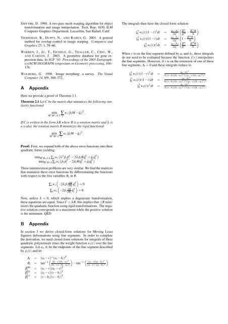
SMYTHE, D. 1990. A two-pass mesh warping algorithm for objecttransformation and image interpolation. Tech. Rep. 1030, ILMComputer Graphics Department, Lucasfilm, San Rafael, Calif.TIDDEMAN, B., DUFFY, N., AND RABEY, G. 2001. A generalmethod for overlap control in image warping. Computers andGraphics 25, 1, 59–66.WARREN, J., JU, T., EICHELE, G., THALLER, C., CHIU, W.,AND CARSON, J. 2003. A geometric database for gene expressiondata. In SGP ’03: Proceedings of the 2003 Eurographics/ACMSIGGRAPH symposium on Geometry processing, 166–176.WOLBERG, G. 1998. Image morphing: a survey. The VisualComputer 14, 8/9, 360–372.A AppendixThe integrals then have the closed-form solution∫ ( )10w i (t)(1−t) 2 dt = |a i−b i | β012∆ 2 i− β 11i βi00i θ i∆ i∫ )10w i (t)t(1−t)dt = |a i−b i |(1− β 012∆ 2 i θ i∆ii∫ ( 10w i (t)t 2 dt = |a i−b i | β012∆ 2 i− β 00i βi11i θ i∆ i).When v is on the line segment defined by a i and b i , these integralsdo not need to be evaluated because the function f(v) interpolatesthe line segments. However, if v is on the extension of one of theseline segments, ∆ i = 0 and these integrals reduce to∫ 10w i (t)(1−t) 2 dt =∫ 10w i (t)t(1−t)dt =∫ 10w i (t)t 2 dt =|a i −b i | 53((v−b i )(b i −a i ) T )((a i −v)(b i −a i ) T ) 3−|a i −b i | 56((v−b i )(b i −a i ) T ) 2 ((a i −v)(b i −a i ) T ) 2|a i −b i | 53((v−b i )(b i −a i ) T ) 3 ((a i −v)(b i −a i ) T ) .Here we provide a proof of Theorem 2.1.Theorem 2.1 Let C be the matrix that minimizes the following similarityfunctionalminM T M=λ 2 I ∑ iw i | ˆp i M− ˆq i | 2 .If C is written in the form λR where R is a rotation matrix and λ isa scalar, the rotation matrix R minimizes the rigid functionalminM T M=I ∑ iw i | ˆp i M− ˆq i | 2 .Proof: First, we expand both of the above error functions into theirquadratic forms yielding(min R T R=I,λ ∑ i w i λ 2 ˆp i ˆp T i − 2λ ˆp i R ˆq T i + ˆq i ˆq T )( imin R T R=I ∑ i w i ˆpi ˆp T i − 2 ˆp i M ˆq T i + ˆq i ˆq T )iThese minimization problems are very similar. We find the matricesthat minimize these error functions by differentiating the functionswith respect to the free variables θ j in R.∑ i w i(−2λ ˆp i∂ R∑ i w i(−2 ˆp i∂ R∂ θ jˆq T i)∂ θ ˆq T j i = 0)= 0Now, unless λ = 0, which implies a degenerate transformation,these equations are equal. Since C= λR, this implies that±R minimizesthe quadratic function using rigid transformations. The negativesolution corresponds to a maximum while the positive solutionis the minimum. QEDB AppendixIn section 3 we derive closed-form solutions for Moving LeastSquares deformations using line segments. In order to completethe derivation, we need closed-form solutions for integrals of threequadratic polynomials times the weight function w i (t) over the linesegments. Let a i , b i be the endpoints of the line segment describedby p i (t) and let∆ i = (a i − v) ⊥ (a i − b i ) Tθ i = tan −1( )(b i −v)(b i −a i ) T− tan −1( )(a i −v)(a i −b i ) T(b i −v) ⊥ (b i −a i ) T (a i −v) ⊥ (a i −b i ) Tβi00 = (a i − v)(a i − v) Tβi01 = (a i − v)(v−b i ) Tβi 11 = (v−b i )(v−b i ) T .