Hyperspectral Vegetation Indices and Their Relationships with ...

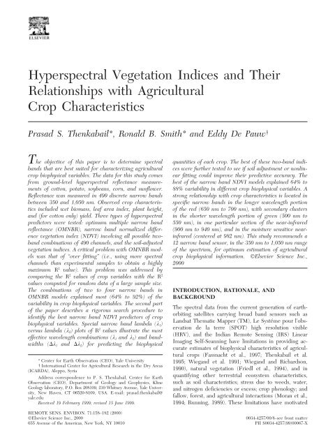
Hyperspectral Vegetation Indices and TheirRelationships with AgriculturalCrop CharacteristicsPrasad S. Thenkabail*, Ronald B. Smith* and Eddy De Pauw †The objective of this paper is to determine spectral quantities of each crop. The best of these two-band indicesbands that are best suited for characterizing agriculturalwere further tested to see if soil adjustment or nonlinbandscrop biophysical variables. The data for this study comes ear fitting could improve their predictive accuracy. Thefrom ground-level hyperspectral reflectance measurementsbest of the narrow band NDVI models explained 64% toof cotton, potato, soybeans, corn, and sunflower. 88% variability in different crop biophysical variables. AReflectance was measured in 490 discrete narrow bands strong relationship with crop characteristics is located inbetween 350 and 1,050 nm. Observed crop characteris- specific narrow bands in the longer wavelength portiontics included wet biomass, leaf area index, plant height, of the red (650 nm to 700 nm), with secondary clustersand (for cotton only) yield. Three types of hyperspectral in the shorter wavelength portion of green (500 nm topredictors were tested: optimum multiple narrow band 550 nm), in one particular section of the near-infraredreflectance (OMNBR), narrow band normalized differ- (900 nm to 940 nm), and in the moisture sensitive nearinfraredence vegetation index (NDVI) involving all possible twoband(centered at 982 nm). This study recommends acombinations of 490 channels, and the soil-adjusted 12 narrow band sensor, in the 350 nm to 1,050 nm rangevegetation indices. A critical problem with OMNBR modelsof the spectrum, for optimum estimation of agriculturalwas that of “over fitting” (i.e., using more spectral crop biophysical information. ©Elsevier Science Inc.,channels than experimental samples to obtain a highly 2000maximum R 2 value). This problem was addressed bycomparing the R 2 values of crop variables with the R 2values computed for random data of a large sample size.The combinations of two to four narrow bands in INTRODUCTION, RATIONALE, ANDOMNBR models explained most (64% to 92%) of the BACKGROUNDvariability in crop biophysical variables. The second partThe spectral data from the current generation of earthofthe paper describes a rigorous search procedure toorbiting satellites carrying broad band sensors such asidentify the best narrow band NDVI predictors of cropLandsat Thematic Mapper (TM), Le Systéme pour l’obsbiophysicalvariables. Special narrow band lambda (k 1 )ervation de la terre (SPOT) high resolution visibleversus lambda (k 2 ) plots of R 2 values illustrate the mosteffective wavelength combinations (k(HRV), and the Indian Remote Sensing (IRS) Linear1 and k 2 ) and bandwidths(kImaging Self-Scanning have limitations in providing ac-1 and k 2 ) for predicting the biophysicalcurate estimates of biophysical characteristics of agriculturalcrops (Fassnacht et al., 1997; Thenkabail et al.* Center for Earth Observation (CEO), Yale University 1995; Wiegand et al. 1991; Wiegand and Richardson,† International Center for Agricultural Research in the Dry Areas(ICARDA), Aleppo, Syria1990), natural vegetation (Friedl et al., 1994), and inAddress correspondence to P. S. Thenkabail, Center for Earth quantifying other terrestrial ecosystem characteristics,Observation (CEO), Department of Geology and Geophysics, Kline such as soil characteristics; stress due to weeds, water,Geology laboratory, P.O. Box 208109, 210 Whitney Avenue, Yale Univer- and nitrogen deficiencies or excess; crop phenology; andsity, New Haven, CT 06520-8109, USA. E-mail: prasad.thenkabail@yale.edufallow, forest, and agricultural interactions (Moran et al.,Received 19 February 1999; revised 15 June 1999.1994; Running, 1989). These limitations have motivatedREMOTE SENS. ENVIRON. 71:158–182 (2000)©Elsevier Science Inc., 20000034-4257/00/$–see front matter655 Avenue of the Americas, New York, NY 10010 PII S0034-4257(99)00067-X

Hyperspectral Vegetation Indices 159the inclusion of hyperspectral sensors onboard the new plants (Blackburn, 1998a, 1998b; Curran et al., 1990),generation of satellites planned by various governments coniferous forest LAI (Gong et al., 1995), pinyon pineand also by the United States private industry (e.g., see canopy LAI (Elvidge and Chen, 1995), and photosynthesisASPRS, 1995; Stoney and Hughes, 1998). The upcomingand stomatal conductance in pine canopies (Carter,narrow band hyperspectral sensors include: (1) Hyperion 1998). The soil-adjusted vegetation index and its numeroussensor with 220 spectral bands, each with 10 nm widemodifications (see Huete, 1988; Qi et al., 1994; Ronsensornarrow bands onboard the National Atmospheric and deaux et al., 1996; Lyon et al., 1998) further improve theSpace Administration’s (NASA) New Millennium Program’sperformance of these indices through “adjustments” forEarth Observer-1 (EO-1); (2) hyperspectral im- soil background effects.aging spectrometer sensor with 105 spectral bands onboardThe indices discussed above involve two bands. Ac-Australian Resource Information Environmental cording to Lawrence and Ripple (1998) and Gong et al.Satellite-1; (3) Warfighter-1 with 200 channels onboard (1995), the use of two-band vegetation indices unneces-ORBVIEW-4 (a U.S. private industry satellite); and (4) sarily constrains the regression analysis. They argue thatmoderate resolution imaging spectrometer (MODIS) if one requires knowledge of an ecological variable (e.g.,with 36 channels (with 10 in visible, six in shortwave in- above-ground biomass or LAI), the researchers must ultimatelyfrared or middle infrared, five in thermal infrared, andanalyze the relationship between the spectral infraredthe rest beyond) onboard Terra (formerly EOS AM-1). dex used and the ecological variable through a regressionThe spectral range of these sensors will be 400 nm to analysis. They and some others (e.g., Shibayama and Aki-2500 nm. Apart from their high spectral resolution, Hyp- yama, 1991; Ripple, 1994) have shown that the piecewiseerion and the Australian sensors also have 30 m spatial multiple regression models performed on discrete nar-resolution. Warfighter-1 will have eight meter resolution. row bands provide flexibility in choosing the bands thatHowever, MODIS has a much coarser spatial resolution, provide maximum information at a given period of cropvarying between 250 m and 1,000 m. All satellites are growth. As the crop conditions vary due to factors suchplanned for launch either during the last quarter of 1999 as management conditions, soil characteristics, climaticor early 2000.conditions, and cultural practices, different band combinationsRecent literature has shown that the narrow bandscan be used (Shibayama and Akiyama, 1991; Shi-may be crucial for providing additional information with bayama et al., 1993).significant improvements over broad bands in quantifyingBased on the above background, the main goal ofbiophysical characteristics of agricultural crops. The this research is to evaluate the performance of varioushyperspectral data for studies reported in literature have types of hyperspectral vegetation indices in characteriz-been gathered using field spectroradiometers (Black- ing agricultural crop biophysical variables. The final goalburn, 1998a; Carter, 1998; Elvidge and Chen, 1995; Shibayamais to determine and recommend an optimal number ofand Akiyama, 1991; Curran et al., 1990), the hyperspectral bands, their centers and widths, in the visi-Compact Airborne Spectrographic Imager (see Gong et ble and NIR portion of the spectrum (350–1,050 nm) real.,1995), and the NASA-designed Airborne Visible-In- quired to best study agricultural crops, thus reducing thefrared Imaging spectrometer (AVIRIS, see Chen et al., redundancy in hyperspectral data. A rigorous and exhaus-1998, Elvidge et al., 1993; Elvidge and Mouat, 1989). In tive approach is adopted in computing and evaluatingthe past three decades, the broad band vegetation indiceshyperspectral indices. Crop variables used are LAI,(VIs) such as TM-derived NDVI have been widely WBM, grain yield, and plant height, which are the bestused to quantify crop variables such as wet biomass indicators of crop growth and yield (see Bartlett et al.,(WBM), leaf area index (LAI), plant height, and grain 1988; Wiegand and Richardson, 1990; Shibayama et al.,yield (see, for example, Tucker, 1979; Wiegand et al., 1993; Thenkabail et al., 1995; Fassnacht et al., 1997).1992; Thenkabail et al., 1995). These broad band indices Biophysical quantities are based on data from five agricultural(e.g., Lyon et al., 1998) use average spectral informationcrops, each with four crop variables.over broad band widths (e.g., TM band 3 or red: 630–690 nm, and TM band 4 or near-infrared: 760–900 nm),resulting in loss of critical information available in specificSTUDY AREAnarrow bands (e.g., Blackburn, 1998a). Also, the The study area is located about 35 km southwest ofNIR and red-based indices are known to be heavily influencedAleppo, Syria. Measurements were taken in farm fieldsby soil background at low vegetation cover (El- that surround this area with the points falling within thevidge and Lyon, 1985; Huete et al., 1985). Further improvementarea encompassed by upper left: 3626 29.5836″ N,in indices is generally possible through use 3635 24.3816″ E; lower right: 3457 46.3428″ N,of spectral data from distinct narrow bands and, further, 3743 47.3736″ E. The Aleppo area is characterized bythrough corrections for soil background effects. These Mediterranean climate: hot and dry summers and coolhyperspectral studies were conducted for rice yield (Shibayamaand wet winters. The annual rainfall varies from 300 mmand Akiyama, 1991), chlorophyll content of to 350 mm. This climate pattern occurs in severalloca-

160 Thenkabail et al.tions in the 30–40-degree latitude belts in both hemi- and topsoil (43 sample locations) (Fig. 1). The meanspheres. The largest single contiguous area experiencing spectral plots of these crops are shown in Fig. 1a throughthis climate is in the Mediterranean basin covering parts d, taking their distinctive growth stages. These growthof West Asia, North Africa, and Southern Europe. Hence phases were (Table 1): early vegetative (potato, soy-a study conducted in such a representative area (Aleppo) beans), late vegetative (soybeans, corn), critical (cotton,has applications across many other Mediterranean rethesoybeans, corn), and yielding/maturing (cotton). Plots ofgions falling within similar climatic, vegetation, and agwillfirst-order derivative spectra (not presented here)ricultural patterns. The overall study area had four soilshow the regions of change and the degree oftypes: very fine clayey chromic calcixerert (the Jindiress change in spectral reflectivity with change in wavelengthregion), very fine clayey calcixerollic xerochrept (Tel Hameasurementsacross the spectrum. At each site, 3 to 10 reflectancewere consistently taken along a transect,dya), clayey calcixerollic xerochrept (Breda), and clayeymixed thermic calcic gypsiorthid (Ghrerife) (Ryan et al., with a nadir view from a height of 1.2 m for cotton, po-1997). During summer, 10% to 20% of the farms in the tato, and soybeans, using a 18 FOV. This resulted instudy area are irrigated from deep wells (recharged byviewing an area of 1,134 cm 2 at the ground level. Typicalaquifers), or by canal irrigation from the Euphratestransact was 30 m to 100 m in length with one spectraat every 10 m interval. For corn and sunflower the view-River. Otherwise most of cultivation is rain-fed duringing height was 1.8 m. Spectroradiometer data of cropsthe winter and spring (November–April).were analyzed using softwares PORTSPEC TM andVNIR TM supplied by the manufacturer of the instrumentMETHODS: COMPUTATION OF(Analytical Spectral Devices TM ), and Statistical AnalysisNARROW BAND INDICES ANDSystem (SAS) version 6.12 (SAS, 1997a, 1997b). The targetreflectance is the ratio of energy reflected off the tar-LABORATORY PROCEDURESget (e.g., crops) to energy incident on the target (mea-Spectral and biophysical data were gathered for five irri- sured using a BaSO 4 white reference). Since the darkgated summer (July–October) crops. All data were coleredcurrent varies with time and temperature, it was gath-lected during a 15-day field campaign in late August andfor each integration time (virtually for each newearly September 1997. A 512 channel spectroradiometer reading). Thus [see Eq. (1)],with a range from 331.8 nm to 1,063.95 nm, manufac-(target-dark tured by Analytical Spectral Devices TM (FieldSPEC, Reflectance (%)(1)(reference-dark current)·1001997), was used to gather spectral data of crops and soils.Due to severe noise in the ends of the spectrum, only Three distinct types of narrow band indices werethe data gathered in 350 nm through 1,050 nm was used, computed using 490 spectral channels of percentage rereducingthe number of spectral channels to 490. The flectance data from the spectroradiometer. The hypersbandcenters were rounded off to nearest whole number pectral indices computed were (see Table 2): (1) all pos-(e.g., 549.86 nm as 550 nm). The spectroradiometer unitsible two-band combination indices involving the 490consisted of a main spectrometer, a personal computer,narrow bands; (2) stepwise linear regression indices in-volving 490 narrow bands; and (3) the soil-adjusted narfiberoptic cable, a pistol grip, and different field of viewrow band indices.(FOV) cones. Inside the spectrometer instrument, lightThe performance of these indices in establishingis projected from the fiber optics onto a holographic difcropcharacteristics (Table 1) were then evaluated andfraction grating where wavelength components are sepacomparedwith the well-known reference Landsat TMrated and reflected for independent collection by the debroadband indices. At each farm, a representative areatector(s) (FieldSPEC, 1997). Five major crops wereof 1 m 2 was chosen for all measurements. At each sampleidentified for spectral and crop biophysical measuresite,two to four sets of reflectance measurements werements. The major crops during this summer period were:taken for one representative plant. The same plant samcotton(Gossypium), potato (Solanum erianthum), soy- ple above the ground was taken for laboratory analysis.beans (Glycine max), corn (Zea mays), and sunflower Above-ground plant height (mm), number of plants in 1(Helianthus). These farms were on four distinct soil m 2 area, and number of rows was recorded. Observationszones. Hence the soil types, color, and transformation were made on the crop growth stage (Fig. 1) and crop(tilled, untilled, fallow) of the soils were noted at each condition. Where farmers were available, planting dateslocation. Spectral reflectance data and quantitative and were recorded that were used in conjunction with cropqualitative data on crops and soils were obtained from growth stages. A digital photograph was taken at each194 locations spread across the study area. The sample site to further supplement the above quantitative anddistribution was: cotton (73 sample locations), potato (25 qualitative observations. Digital photographs providedsample locations), soybeans (27 sample locations), corn valuable additional information on each site, for example,(17 sample locations), sunflower (9 sample locations), in identifying cotton fields that are nearing harvest versus

Hyperspectral Vegetation Indices 161Figure 1. Spectral reflectance characteristics of different crops at distinct growth phases. Sample sizes are shown inside thelegend brackets of each crop.those that are in critical/flowering stages (e.g., Figs. 1a tion of type: NIRa·redb. The slopes (a) and interceptsand b). Photographs also helped in identifying gross mistakes,(b) obtained from the soil lines were used in theif any, in plant density calculations and crop condi- soil adjusted vegetation indices (e.g., narrow bandtion rating. Global Positioning System locations were TSAVI). For further details on methods and proceduresnoted in geographic coordinates (latitude/longitude in refer to Thenkabail et al. (1999).degree, minutes, seconds) and in universal transversemercator (in meters) were recorded. In the laboratory,plant samples were analysed for leaf area (m 2 ), wetRESULTS AND DISCUSSIONweight (kg), and (in the case of cotton) yields (kg lint/ The relationships between the four biophysical variablesha) (Table 1). Leaf area was obtained by running the of five crops and four types of reflectance indices are disleavesover a LI-COR 3100 leaf area meter. The leaf cussed below. Of these, the first index type is broad bandarea obtained from one representative plant is multiplied and the others are narrow band. These indices are:by the number of plants in 1 m 2 area to obtain LAI (m 2 /• broad band TM NDVI (as our reference index);m 2 ). Plants were cut and weighed on a simple weighing• OMNBR reflectance models;machine. This weight was multiplied by number of• two-band NDVI type indices involving all possiplantsin 1 m 2 to obtain biomass (kg/m 2 ). LAI and WBMble combinations of 490 narrow bands; andand plant height measurement were made for all crops• narrow band soil-adjusted vegetation indices.(Table 1). Yield was also obtained for cotton. For thispurpose cotton bolls were counted and converted to kg An overwhelming proportion of the Hyperspectral indexlint per hectare (kg lint/ha) using 600 bolls per 1 kg lint. models indicated that the best relationships were ob-Yields were not gathered for other crops. The mean retionshipstained using LAI or biomass of different crops. The relaflectancevalues obtained for these soils were plotted forwith crop height, yield, and canopy cover alsovarious narrow bands k 1 and k 2 , and fitted using an equa- provided several high R 2 values, but performed poorer

162 Thenkabail et al.Table 1. General Crop Characteristics, Growth Stages and Crop Type DiscriminationGround-Measured Crop VariablesSpectral Vegetation IndicesBroad band Broad band Narrow band Narrow band Narrow bandNDVI (TM4 GVI (TM1, NDVI1 NDVI2 NDVI3plant Canopy and TM3) TM2, TM3, (0.550 lm (0.550 lm (0.920 lmWBM LAI height Yield cover NIR/red and TM4) and 0.468 lm) and 0.682 lm) and 0.696 lm)Crop Growth Stage (kg/m 2 ) (m 2 /m 2 ) (mm) (kg lint/ha) (percentage) (broad band-TM) four-band index green/blue green/red NIR/redCorn critical (11) 2.70 1.50 1471 N/A 100 0.67 44.67 0.39 0.13 0.66Corn late vegetative (6) 2.23 2.06 1105 N/A 85 0.67 38.37 0.45 0.27 0.73Corn (17) all fields 2.53 1.70 1342 N/A 95 0.67 42.45 0.41 0.18 0.68Cotton critical (23) 2.58 1.38 858 1282 95 0.78 49.12 0.39 0.24 0.81Cotton yielding (50) 1.53 0.70 738 1056 85 0.59 41.73 0.25 0.045 0.65Cotton (73) all fields 1.86 0.91 776 1127 88 0.66 44.06 0.29 0.11 0.70Potato early vegetative (17) 0.75 0.34 269 N/A 18 0.54 23.65 0.35 0.004 0.55Potato late vegetative (8) 1.63 0.66 363 N/A 35 0.70 40.40 0.36 0.16 0.72Potato (25) all fields 1.03 0.44 299 N/A 23 0.59 29.01 0.36 0.05 0.60Soybean critical (14) 2.56 3.17 558 N/A 90 0.84 54.52 0.50 0.46 0.88Soybean vegetative (13) 0.40 0.49 204 N/A 40 0.49 24.55 0.41 0.033 0.54Soybeans (27) all fields 1.52 1.84 388 N/A 66 0.67 40.09 0.46 0.22 0.72Sunflower flowering (9) 3.75 2.07 1022 N/A 100 0.73 47.14 0.39 0.33 0.79Distinguishable crops Corn-pot Corn-pot Corn-cot Corn-cot Corn-potCot-pot Cot-pot Cot-pot Corn-pot Corn-sflowerPot-sflower Pot-sbeans Cot-sbeans Corn-sflower Cot-potPot-sflower Cot-sflower Cot-pot Cot-sflowerPot-sbeans Cot-sbeans Pot-sbeansCot-sflower Pot-sflowerPot-sbeansPot-sflowerSbeanssflowerBroad band indices are for Landsat TM bands. NDVI1, NDVI2, and NDVI3 are narrow band indices. NDVI1 has band centers at 0.550 lm (green) and 0.468 lm (blue). GVIgreen vegetationindex of first four TM bands. This is computed using the principal analysis component. See Jackson (1983), Kauth and Thomas (1977), Crist and Cicone (1984), and Wheeler and Misra (1976). TheGVI equation is: GVI0.056710·TM10.008573·TM20.423309·TM30.904168·TM4. Significant differences at 0.10 level or higher for mean vegetation index values between any two crop growthstages of a crop are set in italic. potpotato, cotcotton, sbeanssoybeans, sflowersunflower.

Hyperspectral Vegetation Indices 163Table 2. Indices Used in This StudyVegetation Index Group Vegetation Index Name Abbreviation Definition Reference1. Broad band: Thematic Normalized difference Broad band NIRredRouse et al.Mapper vegetation index (broad band) NDVI NIRred(1973);red: 630–690 nm, NIR: 760–900 nm of Landsat TM sensor(1983)2. Narrow band: multiple Optimum multiple narrow OMNBR This paper (seeaijRjlinear regression band reflectivity (narrow band) J1Table 1)Bi Nwhere Bcrop variable i, Rreflectance in bands j (j1 toNwith N490); athe coefficient for reflectance in band j forith variable.Using MAXR algorithm in SAS (1997a), the best 1, 2, 4, n-variable models are calculated for each crop variablewith equations of the form:a1·NB 1aa1·NB1a2·NB2aa1·NB1a2·NB2a3·NB3a4·NB4 and so on.Where NBnarrow-band and aintercept. The model will usehyperspectral bands 1 to 490 (each band of 1.43 nm wideand spread over 350–1050 nm) and pick a single band providinghighest R 2 value, then finds the two-band combination thatprovides highest R 2 value and so on. aslope or gain ofthe soil line; bintercept or offset of the soil line obtainedby plotting NIR and red bands. Note that these lines aredifferent for the broad bands and narrow bands.3. Narrow band: Normalized difference Narrow band (R jR i )This paper (seenormalized difference vegetation index (narrow band) NDVI narrow band NDVIij (R (RjRi)Fig. 4 andbetween all possible two- where i,j1, N is reflectance (percent) of narrow bands withFig. 5)band combinations of k1 Nnarrow bands490 (each band of 1.43 nm wide andand k 2 (k 1 1 to 490 spread over 350–1050 nm); Rreflectance of narrow bandsbands, k21 to 490bands)4. Narrow band: soil Transformed soil-adjusted Narrow band a·(NIR-a·red-b); aslope and bintercept of soil linesBaret et al.adjusted vegetation index (narrow band) TSAVI (reda·NIR-a·b) (1989)Jackson

164 Thenkabail et al.than LAI and biomass models. Hence, the main focus of and WBM were (Fig. 2a) 0.55 at 910 nm for cotton, 0.51the results presented in this paper will be for LAI and at 910 nm for potato, 0.83 at 825 nm for soybeans, 0.32biomass. Limited results are also presented for other rel- at 940 nm for corn, and 0.53 at 868 nm for sunflower.atively less significant crop variables.Similarly, maximum positive r values between reflectanceHowever, the study begins with a direct evaluation and LAI were (Fig. 2b) 0.51 at 910 nm for cotton, 0.59of the correlation between the single band reflectance at 1025 nm for potato, 0.65 at 854 nm for soybeans, 0.17with biophysical quantities. It was determined during a at 768 nm for corn, and 0.46 at 882 nm for sunflower.preliminary sensitivity analysis that the vegetation indices The 940–1,040 nm moisture sensitive “trough” in percentcomputed for a wide range of the existing sensors such reflectance spectra becomes more significant with increasingas Landsat MSS, Landsat TM, SPOT HRV, NOAAbiomass and crop moisture (Penuelas et al.,AVHRR, and IRS-1C, using simulated data for crops 1993). The trough minima were near 982 nm for mostfrom a spectroradiometer, were highly correlated crops (see Figs. 1a–d). In contrast to the NIR shoulder(R 2 0.95 or higher). Hence computing vegetation indi- (780 nm to 900 nm), in which spectral reflectanceces for any one of these sensors will provide nearly the changes only marginally for all crops (except cotton andsame information as similar indices computed for other corn), the visible portion of the spectrum (400–700 nm)sensors. Elvidge and Chen (1995) determined that the is highly sensitive in different discrete portions in blue,relatively narrower bands of TM and MSS sensors green, and red, as evident in Fig. 1. This characteristicshowed only slight improvements over broader bands resulted in a rapidly changing correlation coefficient be-from sensors such as AVHRR. Therefore, the TM NDVI tween crop biophysical variables (WBM and LAI) and(see Table 2) was the only broad band index computed spectral reflectance for a given crop in 400–700 nm comandreported throughout this paper. The discrete 1.43 pared to the relatively uniform r values in 780–900 nmnm wide narrow band reflectance data obtained using (Fig. 2).the spectroradiometer were averaged over the spectralbands 760 nm to 900 nm (for TM band 4) and 630 to OMNBR Reflectance Relationships with690 nm (for TM band 3) to obtain broad band NDVI Crop Variablesfor each data point.The OMNBR reflectance indices (see Table 2), were relatedto crop biophysical variables through stepwise lin-Single Narrow Band Reflectance Relationships ear regression analysis. The dependent variables (B i )inwith Crop Variablesthe model are crop variables and independent variablesAs a first step, reflectance in the 490 individual narrow are reflectances (R j ) in the 490 discrete narrow bands.bands was correlated with crop biophysical variables: Of several statistical methods available to run piecewiseWBM and LAI of all the five crops (Fig. 2). Maximum linear regression models, the stepwise MAXR procedurenegative correlation coefficients (r) in the red band por- (SAS, 1997a, 1997b) is considered the best and hence istion were mostly centered around 680 nm. This is a regionused in this study. Using the MAXR procedure, theof high chlorophyll absorption in green vegetation. model providing the highest R 2 value for one-, two-, andThe maximum negative r values for relationships betweenfour-variable OMNBR models were determined for deforreflectance and WBM were (Fig. 2a) at 682 nm veloping relationships with WBM, LAI, and plant heightcotton (r0.75), potato (0.47), soybeans (0.72), of four crops (cotton, potato, soybeans, and corn), as welland corn (0.41) (Fig. 2a). For sunflower it was cen- as yield of cotton crop (Table 3). In 10 of 13 biophysicaltered at 625 nm (r0.58). There were similar trends variables, the first four narrow band variables explainedwith LAI (Fig. 2b). Around 700 nm, the amount of en- 76% or above variability (Table 3). This is nearly theergy reflected off green vegetation begins to increase. same percentage of variability explained when the ratioThe wavelength portion 700 nm to 780 nm has the high- of the number of independent variables or number ofest change in reflectance per unit change in wavelength bands (M) to that of the total number of field samplesin all of the visible and NIR portion of the spectrum, (N) for that variable is between 0.15 and 0.20 in differentreaching a peak around 780 nm (see Fig. 1). The r values crop variables (see Fig. 3). As M approaches N, the R 2change dramatically from negative around 682 nm to value approaches 1. Beyond M/N of 0.15 to 0.20 (seepositive around 740 nm for biomass (Fig. 2a) and LAI Fig. 3), there were only small increases (often statistically(Fig. 2b) for all crops. In the 740 nm to 875 nm portion insignificant) with addition of another variable. This featureof the spectrum, r values for WBM and LAI are highhas been illustrated in Fig. 3 for the relationshipsand nearly constant. Beyond 875 nm, other crop specific between narrow bands and LAI of four crops by comparingrelationships are seen. For example, maximum r valuesthem with idealised random (RAND in Fig. 3) plot,for cotton crop reflectance with: (1) WBM was 0.55 at which shows the nature of the curve when the sample910 nm (Fig. 2a), and (2) LAI was 0.51, also at 910 nm sizes are large (350 in this case). For each crop, the R 2(Fig. 2b). Maximum positive r values between reflectance values were statistically significant for the one-variable

Hyperspectral Vegetation Indices 165Figure 2. Correlation coefficients (r) between spectral reflectance in the 512 discrete channelsand biophysical variables of the five crops for (a) WBM and (b) LAI.models and increased significantly with the addition of a band, M, index exceeds the threshold M/N value of 0.20.)second, third, and, at times, the fourth variable (Fig. 3 These results compare well with Blackburn (1998a), whoand Table 3). Four-variable models explained 64% to mentions that there is a likelihood of the multiple narrow92% variability in crop biophysical variables, significantly band models being “over-fit” and hence the relationshipshigher than 53% to 81% by two-variable models, and need to be validated using independent datasets.18% to 69% by one-variable models (Table 3). Beyond The first two bands, typically, constitute a red andthe fourth variable, the increases with addition of each NIR, a red and a green or a red-edge and a NIR bandvariable is small and statistically insignificant. A quality combinations (see bands of two-variable models in Tablefactor (QR 2 crop/R 2 rand) demonstrates that the statistical 3). In four-variable models the bands that occur mostsignificance of the extra information decreases as more clustered in the longer wavelength portion of red (651channels are added. For example, Q for the first five val- nm to 700 nm), moisture-sensitive NIR (951 nm to 1000ues of cotton crop were 3.38, 2.50, 1.93, 1.89, and 1.81. nm), shorter wavelength portion of green (501 nm to 550The first two-variables explain most of the variability. nm), and longer wavelength portion of NIR (900 nm toAny increase in R 2 beyond M/N0.15–0.20 is an mathematical940 nm). This result suggests the fact that the optimalartefact arising from limited sample size com- information on crops is not necessarily concentrated inpared to the number of channels in a hyperspectral sensor.the red and NIR wavelengths. The waveband combina-(Note: for corn with only 17 samples, N, even a four- tions providing optimal information are dependent ona

166 Thenkabail et al.Table 3. Optimum Multiband predictorsBest One-Variable Best Two-Variable Best Four-VariableModel OMNBR Model OMNBR Model OMNBRBest R 2 Value for Two-BandNormalized DifferenceVegetation Index Models(Results from Table 4)Band centers Band Centers Band CentersDependent (nm) (nm) (nm) Broad Band Narrow BandPercent Increase in Four BestVariable ModelCrop Type Crop (Independent (Independent (Independent NDVI Model NDVI Model Broad Band Narrow Band(Sample Size) Variable Variable) R 2 Variables) R 2 Variables) R 2 R 2 R 2 NDVI NDVI1. Cotton (73) except for WBM 682 0.56 682,910 0.75 368,668,925,968 0.79 0.76 0.79 3 0yield for which the LAI 682 0.44 682,910 0.60 353,682,925,968 0.70 0.61 0.66 11 4sample size is 49 Plant height 910 0.40 682,925 0.53 668,696,910,982 0.64 0.41 0.52 23 10yield 954 0.52 696,968 0.73 525,582,668,968 0.77 0.54 0.64 23 132. Potato (25) WBM 910 0.26 711,954 0.68 511,682,711,940 0.80 0.67 0.76 23 4LAI 1025 0.34 668,1025 0.67 525,568,682,997 0.80 0.78 0.88 2 8Plant height 910 0.31 668,910 0.60 425,539,568,668 0.83 0.68 0.77 15 63. Soybeans (27) WBM 825 0.68 725,811 0.76 353,754,811,825 0.81 0.79 0.84 12 3LAI 682 0.47 668,682 0.61 668,682,811,954 0.76 0.72 0.80 4 4Plant height 825 0.69 739,811 0.81 525,739,754,982 0.92 0.75 0.78 17 134. Corn (17) WBM 654 0.30 511,654 0.69 439,511,625,954 0.78 0.59 0.71 19 7LAI 682 0.43 482,982 0.60 410,496,511,1025 0.78 0.70 0.86 9 8Plant height 1025 0.18 725,1025 0.39 525,568,725,1025 0.66 0.26 0.31 40 38Piecewise OMNBR models were obtained using MAXR algorithm in SAS (1997a and 1997b). The model with highest R 2 between OMNBR (four-variable), narrow band NDVI and broad bandNDVI is shown in bold. Bandwidths are 1.43 nm wide for each band center. Band centers in fraction were rounded off to nearest whole number (e.g., 549.86 nm as 550 nm.

Hyperspectral Vegetation Indices 167Figure 3. Plot of the ratio M/N versus R 2 value.host of variables, such as crop growth stage, crop condi- ous to be presented here) were created for all the othertion, and cultural practices. An interesting result in Table biophysical variables of each crop.3 is the frequent appearance of narrow bands from the Based on the above results, band centers (k 1 and k 2 )visible portion (400 nm to 700 nm) apart from the longer and band widths (k 1 and k 2 ) that combine to form thewavelength portion of NIR and the moisture-sensitive best seven indices (ranked based on R 2 values) were determinedNIR. The visible spectrum is very sensitive to loss offor WBM and LAI of cotton, potato, soybeans,chlorophyll, browning, ripening, and senescing (Idso et corn, and for the pooled data of all crops (Table 4). Theal., 1980), variations in carotenoid (Blackburn, 1998b; band centers and their widths are identified for the LAI,Tucker, 1977) and soil background effects. The visible WBM models of each crop variable. This can be determinedspectrum is highly sensitive to crop senescence rates andthrough k 1 and k 2 contour plots of R 2 values (Figs.is generally an excellent predictor of grain yield (Idso et 4 and 5). We determined that a contour interval of 0.05al., 1980). This study showed that the most sensitive portionfor R 2 values provide a reasonable and statistically soundof bands to predict senescing cotton (sample size 50) approach of arriving at band centers and band widths.yield were predominantly in the visible red narrow bands Smaller contour intervals result in several more gradients(centered at 696 nm or 668 nm) and moisture-sensitive of R 2 values, providing other band centers and bandNIR (968 nm and/or 954 nm) (see these bands in one- widths. These can be too numerous and often providevariable, and/or two-variable, and/or four-variable models no significant statistical difference between two discretein Table 3).contour intervals. For example, the index that has highestcorrelation for cotton WBM has band centers (k 1 andNarrow Band NDVI Relationships withk 2 ) and bandwidth (k 1, and k 2 ) extracted from the con-Crop Variables tour plot range of 0.70 to 0.75 (highest R 2 value range)The availability of hyperspectral data in 490 (N) discrete in the lower diagonal portion of Fig. 4. The band centersnarrow bands allowed computation of NN240,100 and bandwidths are (Fig. 4): k 1 682 nm (k 1 28 nm),narrow band NDVIs for any one crop variable (Table 2). and k 2 918 nm (k 2 20 nm). These band centers andRegression coefficients R 2 between all possible two-band widths are then tabulated in Table 4. The same rangenarrow band vegetation indices and crop biophysical varitinctive(0.70 to 0.75) of contour intervals can be split into dis-ables were determined. The result of this comprehensivegroups of smaller intervals such as 0.70 to 0.72,analysis is illustrated in contour plots of the R 2 values, 0.73 to 0.74, and 0.74. Then it is possible to derivefor each k 1 and k 2 pair, in Figs. 4 and 5. It suffices to band centers (k 1 and k 2 ) and bandwidths (k 1 and k 2 )display the matrix only below (or above) the diagonal of to each one of these smaller intervals. However, the sig-the matrix as the R 2 (k 1 and k 2 ) values are symmetrical. nificance of the band centers and bandwidths from theFurther, in both these figures, only R 2 values above 0.4 small intervals of R 2 values, such as between 0.70 to 0.72are plotted for clarity. Similar contour plots (too numer- and 0.73 to 0.74, is limited since these R 2 values did not

168 Thenkabail et al.Figure 4. Contour plot showing the correlation (R 2 ) between WBM and narrow band NDVI valuescalculated for 490 narrow bands spread across k 1 (350 nm to 1050 nm) and k 2 (350 nm to 1050 nm). Thedifferent areas of “bulls-eye” are the regions with high R 2 values, which were ranked and from which bandcenters (k 1 and k 2 ) and band widths (k 1 and k 2 ) were calculated for the seven best indices of each cropvariable, as in Table 5.have significant statistical difference or were statistically (which has a 0.05 R 2 value contour interval). An evaluationdifferent only at 0.10 level or higher. Therefore, the k 1of these results for various crop variables show a redifferentand k 2 spectral band combinations obtained from the dis- markably strong relationships centered in the longer portiontinctive contour intervals of 0.05 were considered a reasonableof red, 650 nm to 700 nm, a particular portion ofand statistically sound approach. The second best NIR, 900 nm to 940 nm, and shorter portion of theindex (index with second highest correlation) is then selectedgreen band, 500 nm to 550 nm (see specific narrow bandfrom the contour plot region with R 2 value range centers and their widths in Table 4 and the clusters inof 0.65 to 0.70. Following a similar procedure, band centersFig. 6). For the precise R 2 values, visually scan throughand bandwidths of the seven best indices for a par- 490 (N) by 490 (N) matrix of R 2 values. Identify the k 1ticular crop variable is determined (Table 4). Similar procedureand k 2 band centers having highest R 2 value. This is theis adopted for determining k 1 , k 2 , k 1 , and k 2 band center for the index, which has highest correlation.for indices of other crop variables and for the pooled Observe the R 2 values in the immediate vicinity of thesedata of all crops (Table 4). When visually inspecting the band centers (k 1 and k 2 ). Often the R 2 values remain thecontour plots of R 2 values, it must be noted that more same or nearly the same for a few narrow bands in im-precise bandwidths are possible with a smaller range of mediate vicinity of k 1 and k 2 . This range of similar orcontour interval plots of R 2 values than shown in Fig. 4 near-similar spectral response to a crop variable will con-

Hyperspectral Vegetation Indices 169Figure 5. Contour plot showing the correlation (R 2 ) between LAI and narrow band NDVI values calculatedfor 490 narrow bands spread across k 1 (350 nm to 1050 nm) and k 2 (350 nm to 1050 nm). The different areasof “bulls-eye” are the regions with high R 2 values, which were ranked and from which band centers (k 1and k 2 ) and band widths (k 1 and k 2 ) were calculated for the seven best indices of each crop variable, asin Table 5.stitute the bandwidth. Bandwidths can also be assessed and k 2 ) determined for the seven best linear modelsby systematically increasing bandwidth centered over a (Table 4) were used for computing nonlinear exponentialwavelength (at 1 nm or 2 nm steps) or using prespecified models. The R 2 values for the seven best linear and nonbandwidths.However, the approach adopted in this pa- linear exponential narrow band vegetation index modelsper is more comprehensive when compared to these ap- were computed and listed for each biophysical variableproaches.(Table 5). The best hyperspectral models for WBM explained79% variability for cotton, 76% variability for po-Narrow Band Nonlinear Model Relationships with tato, 84% variability for soybeans, 71% variability forCrop Variablescorn, and 59% variability for all crops Table 5). Similarly,Figures 4 and 5 depict R 2 values for linear relationships the best LAI models explained 66% variability for cotton,between crop biophysical variables and hyperspectral in- 88% variability for potato, 80% variability for soybeans,dices. However, most relationships between crop bio- 86% variability for corn, and 65% variability for all crops.physical variables and spectral indices are nonlinear. It Except in three cases, nonlinear models performed sub-was noticed in this study that overwhelming proportions stantially better than the linear models. However, inof the best nonlinear models were exponential (e.g., Fig. three cases (corn WBM, corn LAI, and cotton yield) lin-7). The band centers (k 1 and k 2 ) and band widths (k 1 ear models performed better than the nonlinear models.

170 Thenkabail et al.Table 4. Seven best NDVIs. Band Centers (k 1 and k 2 ) and Band Widths (Dk 1 and Dk 2 ) in nm for the Linear Narrow bandNDVI Models for the Different Crop VariablesBand Centers (k 1 and k 2 ) and Band Widths (k 1 and k 2 ) for Two-BandBand CenterVegetation IndicesCrop Crop and Width Index 1 Index 2 Index 3 Index 4 Index 5 Index 6 Index 7(Sample Size) Variable (nm) (nm) (nm) (nm) (nm) (nm) (nm) (nm)1. Cotton (73) WBM k 1 682 682 568 555 615 525 982except for (kg/m 2 ) Dk 1 28 28 10 20 175 4 10yield that (see Fig. 4) k 2 918 845 918 666 925 540 940has a sample Dk 2 20 250 10 5 20 7 10size of 50 LAI k 1 682 550 678 550 568 525 940(m 2 /m 2 ) Dk 1 15 30 15 50 4 60 10k 2 940 682 865 675 915 540 980Dk 2 60 20 275 50 15 60 10yield (lint/ha) k 1 540 696 678 540 690 678 670Dk 1 30 4 30 40 10 30 50k 2 678 940 940 684 720 860 970Dk 2 20 20 50 20 20 290 202. Potato (25) WBM k 1 550 550 678 682 720 682 615(kg/m 2 ) Dk 1 20 30 10 20 30 10 70k 2 682 682 920 940 790 710 935Dk 2 4 26 20 40 20 20 50LAI (m 2 m 2 ) k 1 682 472 682 678 550 682 625(see Fig. 5) Dk 1 28 15 28 28 20 7 50k 2 982 790 738 860 688 940 940Dk 2 36 20 45 100 28 30 83. Soybean (27) WBM k 1 725 732 696 565 550 635 490(kg/m 2 ) k 1 25 10 28 50 20 30 75(see Fig. 4) k 2 845 758 791 875 755 682 682k 2 70 10 10 130 10 10 28LAI (m 2 /m 2 ) k 1 625 495 495 730 682 690 418Dk 1 30 30 30 20 10 40 510k 2 688 685 670 840 790 860 855Dk 2 15 20 40 60 20 100 904. Corn (17) WBM k 1 720 505 715 620 620 620 490(kg/m 2 ) Dk 1 18 10 4 30 30 30 50k 2 820 645 990 830 1.000 940 825Dk 2 160 6 20 160 30 70 110LAI k 1 620 550 635 470 495 495 650(m 2 /m 2 ) Dk 1 20 30 20 8 50 50 4(see Fig. 5) k 2 590 684 720 740 760 1.000 800Dk 2 10 28 10 2 40 25 1655. All crops WBM k 1 682 655 525 660 525 640 510(151) a (kg/m 2 ) Dk 1 30 90 20 30 50 120 100k 2 910 920 682 875 675 880 670Dk 2 20 20 25 250 30 280 60LAI (m 2 /m 2 ) k 1 540 682 550 682 682 670 490Dk 1 20 10 40 28 35 40 30k 2 682 756 682 910 754 910 965Dk 2 10 20 30 200 40 200 20Indices are arranged in order of ranking (higher the R 2 value higher is the ranking) and obtained from k 1 and k 2 contour plots of R 2 values (see,for example, Figs. 4 and 5). The R 2 values of these models are listed in Table 4.aIncludes nine samples from sunflower crop in addition to the cotton (73), potato (25), soybeans (27), and corn (17).All corn fields were either in late vegetative or critical crop variable to determine if soil adjustment improves R 2growth phases (Fig. 1d) resulting in a narrow dynamic values of the crop models. The TSAVI performed betterrage of their indices. In comparison, cotton, soybeans, than the other soil-adjusted indices (see Qi, 1994; Ronandpotato had distinctive growth stages (Fig. 1), provid- deaux et al., 1996; Huete, 1988) and hence is the onlying data over a larger dynamic range.soil-adjusted index reported. TSAVI requires site-specificsoil line slopes (a) and intercepts (b) (see Lawrence andNarrow Band Soil-Adjusted Vegetation Index Ripple, 1998). In this study, a and b are computed usingRelationships with Crop Variablesdata from 43 soil samples, covering four soil types, byThe narrow band TSAVI indices (Table 2) were computedplotting the spectra of two bands (k 1 and k 2 ) involved infor the best narrow band NDVI indices of each best indices and performing best-fit regression. Ourre-

Hyperspectral Vegetation Indices 171Figure 6. Percentage of occurrences of hyperspectral narrow bands in the three best NDVI models and in three best narrowband four-variable multiple linear models (OMNBR models).search supports the concept that a well-defined soil line were in early vegetative growth phases with about 40%exists for NIR and red. However, there is also a “soil canopy cover, with the rest having about 90% canopyline” for other wavebands such as between green and red cover (Fig. 1c). These conditions resulted in potato(Thenkabail et al. 1999) and other wavebands like rededgeWBM showing the highest increase in R 2 value (5%) forand NIR.the narrow band TSAVI models over the best narrowExcept in the case of potato WBM, and to a much band NDVI models. Generally, soil background effectslesser extent soybean LAI, the increase in R 2 value in can be reduced using indices such as TSAVI (Elvidgesoil-adjusted models over the other narrow band NDVI and Chen, 1995), especially for agricultural crops or ho-models were insignificant. Potato and soybeans were the mogeneous plant canopies (Rondeaux et al., 1996). However,two crops with the highest soil background influences.the soil-adjusted vegetation indices are more signiftwoBoth of these crops were samples within two very dis- icant when agricultural crops are studied on widelytinct growth stages (see Figs. 1b and c). Of the 25 potato varying soils (see, for example, Lawrence and Ripple,fields, for example, 17 were in early vegetative and eight 1998). The four soil types in this study area had fine orwere in middle or late vegetative (Fig. 1b). The growth very fine clayey Calcixerollic Xerochrept and Chromicstages were identified in the field by experts. The 17 Calcixerert. It is likely that the improved sensitivity ofcornfields had about 18% canopy cover. Even the late these indices become apparent when diverse soil typesvegetative fields had only about 35% canopy cover. Be- are studied.low 25% to 35% canopy cover, soil background reflectanceFor cotton yield, the soil-adjusted index explainedis the principal contributor to overall spectral re- 9% less variability compared to the corresponding nar-sponse (Tueller, 1987). Of the 27 soybeans fields, 13 row band index. This could be attributed to mix of spec-

172 Thenkabail et al.Figure 7. Comparison between the broad band and the narrow band soil-adjusted indices for potato WBM (a and b), and soybeans LAI(c and d). NIR and red-based indices of broad bands (a and c) versus visible band based indices of narrow bands (b and d).

Hyperspectral Vegetation Indices 173Table 5. R 2 Values of the seven-best NDVIs Reported in Table 3HyperspectralPercent Increase (Positive) orDecrease (Negative) of the BestNarrow Band TSAVI overIndices (lm/lm) Linear Model Nonlinear Percent Increase The Best(Narrow band R 2 of Exponential Model of the Best Soil-Adjusted The best The bestCrop Parameter NDVI Model (Narrow Band R 2 of (Narrow Band Narrow Band R 2 Narrow Broad-band Narrow-bandUnits, (Sample Size) Ranking) NDVI—linear) NDVI—Nonlinear) NDVI over OMNBR Band TSAVI NDVI NDVI1. Cotton WBM 1 0.72 0.79 3 0.80 4 1(kg/m 2 , 73) 2 0.68 0.723 0.66 0.714 0.67 0.675 0.64 0.676 0.60 0.577 0.56 0.56TM-NDVI 0.70 0.762. Cotton LAI 1 0.59 0.66 5 0.67 6 1(m 2 /m 2 , 73) 2 0.59 0.633 0.53 0.584 0.53 0.575 0.48 0.526 0.44 0.487 0.41 0.43TM-NDVI 0.53 0.613. Cotton yield 1 0.64 0.62 10 0.55 1 9(Lint/ha, 50) 2 0.61 0.573 0.59 0.504 0.54 0.535 0.54 0.456 0.50 0.417 0.46 0.40TM-NDVI 0.54 0.514. Soybeans WBM 1 0.73 0.84 5 0.84 5 0(kg/m 2 , 27) 2 0.71 0.843 0.68 0.824 0.68 0.785 0.68 0.786 0.68 0.757 0.65 0.79TM-NDVI 0.59 0.79(continued)

174 Thenkabail et al.Table 5. (continued)HyperspectralPercent Increase (Positive) orDecrease (Negative) of the BestNarrow Band TSAVI overIndices (lm/lm) Linear Model Nonlinear Percent Increase The Best(Narrow band R 2 of Exponential Model of the Best Soil-Adjusted The best The bestCrop Parameter NDVI Model (Narrow Band R 2 of (Narrow Band Narrow Band R 2 Narrow Broad-band Narrow-bandUnits, (Sample Size) Ranking) NDVI—linear) NDVI—Nonlinear) NDVI over OMNBR Band TSAVI NDVI NDVI5. Soybeans LAI 1 0.69 0.80 8 0.82 10 2(m 2 /m 2 , 27) 2 0.61 0.773 0.55 0.764 0.53 0.685 0.52 0.756 0.46 0.737 0.46 0.73TM-NDVI 0.45 0.726. Potato WBM 1 0.68 0.76 9 0.81 14 5(kg/m 2 , 25) 2 0.67 0.723 0.61 0.754 0.57 0.695 0.56 0.656 0.54 0.727 0.49 0.65TM-NDVI 0.50 0.677. Potato LAI 1 0.67 0.88 10 0.89 11 1(m 2 /m 2 , 25) 2 0.67 0.883 0.65 0.874 0.63 0.875 0.58 0.866 0.55 0.807 0.49 0.82TM-NDVI 0.50 0.788. Corn WBM 1 0.71 0.59 12 0.70 11 1(kg/m 2 , 17) 2 0.69 0.473 0.65 0.524 0.59 0.485 0.59 0.436 0.54 0.397 0.47 0.34TM-NDVI 0.59 0.52(continued)

Hyperspectral Vegetation Indices 175Table 5. (continued)HyperspectralPercent Increase (Positive) orDecrease (Negative) of the BestNarrow Band TSAVI overIndices (lm/lm) Linear Model Nonlinear Percent Increase The Best(Narrow band R 2 of Exponential Model of the Best Soil-Adjusted The best The bestCrop Parameter NDVI Model (Narrow Band R 2 of (Narrow Band Narrow Band R 2 Narrow Broad-band Narrow-bandUnits, (Sample Size) Ranking) NDVI—linear) NDVI—Nonlinear) NDVI over OMNBR Band TSAVI NDVI NDVI9. Corn LAI 1 0.86 0.68 16 0.87 16 1(m 2 /m 2 , 17) 2 0.80 0.563 0.77 0.504 0.71 0.475 0.68 0.476 0.68 0.457 0.63 0.45TM-NDVI 0.70 0.5910. All Crops 1 0.43 0.59 5 0.59 5 0WBM (kg/m 2 , 151, 2 0.41 0.58including nine 3 0.39 0.54for sunflower) 4 0.39 0.525 0.38 0.496 0.35 0.497 0.35 0.45TM-NDVI 0.40 0.5411. All crops 1 0.54 0.65 6 0.65 6 0LAI (m 2 /m 2 , 151, 2 0.48 0.64including nine 3 0.40 0.63for Sunflower) 4 0.38 0.615 0.38 0.596 0.37 0.597 0.29 0.38TM-NDVI 0.39 0.59The R 2 values for the linear and nonlinear hyperspectral narrow band NDVI models and their comparison with: (a) soil-adjusted narrow band TSAVI models and (b) broad band NDVI (TM-NDVI) models.

176 Thenkabail et al.tral signature from the cotton lint, cotton leaves that arechanging color from green to light green or yellowishgreen, exposed cotton stems (as a result of falling leaves),and some soil background. The narrow band TSAVImodels use slopes and intercepts of the soil line to correctfor soil background influences only. However, whenother factors (e.g., lint, stem, and different shades ofleaves) become prominent, the soil adjustment can reducethe accuracy of the prediction.Discrimination of Crop Types and Growth StagesA knowledge of crop growth stages and crop types (Fig.1, Table 1) is critical in understanding the reflectivity ofdifferent portions of the spectrum. To illustrate this, twoTM indices (broad band NDVI and broad band GVI),and three hyperspectral indices (a green and a blueband-based index: narrow band NDVI1; a green and ared band-based index: narrow band NDVI2; and a redand NIR-based index: narrow band NDVI3) were used(Table 1). Statistical tests of significances were performedon mean vegetation indices of the distinctivegrowth stages (Table 2). The essential notion is that thedistribution of sample data may be used to attach confidencelevels to spectrally separable classes (Wallace andCampbell, 1989). The mean broad band NDVI for corn(0.67) and cotton (0.66) were about the same (Table 1).Similar insensitivity was detected even when the fourTM bands were used in broad band GVI, which providedvalues of 42.45 for corn and 44.06 for cotton. Incomparison, narrow band NDVI1 involving two visiblebands provided significant statistical differences (at 95%confidence level) for corn (0.41) and cotton (0.29). Similar,results were obtained using narrow band NDVI2 involvingtwo other visible bands, which had mean valuesof 0.18 for corn and 0.11 for cotton. Further, the magni-Other IndicesWhen a difference index is formulated using two closelyspaced band centers, it is indicative of the slope of thereflectance with respect to wavelength and is often re-ferred to as a derivative vegetation index (see Elvidgeand Chen, 1995). The “bullseye” areas in Figs 4 and 5,which are on the diagonal, are ideal for computing hyp-erspectral derivative indices. The first- and second-orderderivative spectra (Elvidge and Chen, 1995) were also investigated.The best derivative indices in this study ex-plained 35% to 86% variability in different crop variables,but overall performed significantly poorer than thenarrow band and most broad band indices discussed inthe previous sections. Hence it is not necessary to reportthese results in detail. There are indications that the de-rivative indices are more sensitive to changes in sparselyvegetated and complex (mixture of green and brown)grassland canopies (Elvidge and Chen, 1995; Curran etal., 1990) rather than for crop canopies.tude of differences in one or the other narrow band indiceswere often higher than broad band NDVI indices.For example, broad band NDVI indices provided significantdifference between soybeans (0.67) and potato(0.73) (Table 1). This difference increased when narrowband NDVI2 (0.22 for soybeans and 0.33 for sunflower).Overall, the narrow band NDVI2 provided significantdifference between nine combinations of crop types(corn-cotton, corn-potato, corn-sunflower, cotton-potato,cotton-soybean, cotton-sunflower, potato-soybean, potato-sunflower,and soybean-sunflower). In comparison,narrow band NDVI1 provided significant difference foronly five combinations, and narrow band NDVI3 with sixcombinations (Table 1). Compared to this the broadband indices provided significant difference betweenonly three or four combinations of crops. Similar trendscan be observed for the growth stages. For example, thebroad band NDVI indices were about the same for cornin critical (0.67) and corn in late vegetative (0.67) (Table1). Compared to this narrow band indices in Table 1show dramatically improved sensitivities. These resultsimply that through the use of indices derived from vari-ous narrow bands it is possible to maximize crop infor-mation. Often information is captured at a specific nar-row band better than the other portions depending onphenological and physiographic variability. The resultshere showed narrow bands centered at 0.550, 0.682,0.696, 0.920, and 0.468 as most critical for discriminat-ing crops.Dynamic Range and Saturation of IndicesThe “saturation” or upward curvature in plots of WBMor LAI versus a two-band vegetation index is a wellknownproblem (e.g., Wiegand et al. 1992; Huete et al.,1985). It limits the predictive accuracy of the regressionequations. Our own data, as explained in the followingparagraphs, shows this behavior strongly. The acceptedexplanation for saturation is that in dense vegetation, theleaf coverage approaches 100%, while the biomass andLAI continue to grow. Typically, crops reach 100% canopycover around mid-vegetative phases. However, almostall crops continue to accumulate biomass and LAIuntil they reach critical phases of growth at which pointthey begin to senesce. NDVI saturates at LAI of 2.5 to3 because the amount of red light that can be absorbedby leaves rapidly reaches a peak. In contrast, NIR scatteringby leaves continues to increase even as LAI exceeds3. As a result, once a canopy reaches 100%, NIRreflectance will continue to rise but red reflectance willshow only modest decreases, resulting in only slightchanges in the ratio (the denominator will have a muchgreater impact on the ratio than the numerator). For ex-ample, consider a canopy that has reached 100%. Redreflectance might be as low as 2%, while NIR could beas high as 50% to 60% depending on the crop (and can-

Hyperspectral Vegetation Indices 177opy structure). This would lead to an NIR/red ratio of fects (litter, weeds), are important, requiring further research25 or 30. An increase in LAI might lead to a very slightin explaining the question of saturation.decrease in red (say to 1.8%) because most of the redreflectance is coming from upper layers of leaves, which Frequently Occurring Optimum Bandshave already absorbed all of the light they can. In con- To gain a broad view of the results in this paper, it istrast, NIR reflectance would still increase because leaves useful to consider bands that frequently appear in optiarehighly transmittant in the NIR and thus additional mum indices. It can be said that these bands contain anleaves will still impact NIR scattering. NIR reflectance overwhelming fraction of the total crop information inmight still show a substantial increase (say to 55% to the full spectrum.65%) but only generate a modest increase in the ratio The results obtained using narrow band NDVI models(30 to 35), because little change has occurred in the dereflectance(e.g., Tables 4 and 5, Figs. 4 and 5) and OMNBRnominator. In order to double the ratio, NIR reflectancemodels (e.g., Table 3) were used for denominator.would have to nearly double to compensate for little termining the band centers and widths (see Fig. 6 andchange in red reflectance. Because of this, the indices Table 6) for estimation of crop biophysical variables. Thethat have the best chance for overcoming saturation are procedure of obtaining the band centers and band widthslikely to have red bands, especially in the narrow band was explained previously. The narrow bands that appearportion where red absorption is maximum (an anonyindexin two-band NDVI type models ranked 1, 2, and 3 (seemous reviewer contributed to much of this paragraph).1, 2, and 3 in Table 4) and the narrow bands thatThe broad band NIR and red-based indices often occur in 1-variable, 2-variable, and 4-variable OMNBRhave serious problems of saturation. This can be seen in models (Table 3) of different crops were evaluated (Fig.the models of potato WBM (Fig. 7a) and to still greater 6). The percentage of these narrow bands in every 50extent in soybean LAI (Fig. 7c). For potato (Fig. 7a), nm interval were established and their clusters plottedwhen WBM is less than 0.7 m 2 /m 2 there is a proportional for the 350 nm to 1050 nm (Fig. 6). In both model types,increase in NDVI, showing a clear linear trend. Beyond an overwhelming proportion of crop information was inthis value the trend of the plot becomes nonlinear. For the longer red (650 nm to 700 nm), a particular portionsoybeans (Fig. 7c), when LAI is less than 1.0 m 2 /m 2 there of NIR (900 nm to 950 nm), and a portion of green (500is an proportional increase in NDVI, but beyond this the nm to 550 nm). These were followed by the shorter halftrend becomes nonlinear, reaching a plateau around LAI of NIR shoulder (800 nm to 850 nm), red-edge (701 nmof 3.0 m 2 /m 2 . In such cases, hyperspectral data offers op- to 750 nm), and the moisture-sensitive NIR (951 nm toportunity to scout for band combinations that: (1) offer 1000 nm) (Fig. 6). A remarkable 36.4% of all the bandsthe best two-band-based NDVI type of relationships (see that occur in the first-, second-, and the third-best mod-Figs. 4 and 5) that are often different from the widelyels of narrow band NDVI type models were clustered inused NIR and red-based indices; or (2) perform stepwise651 nm to 700 nm region of the spectrum (Fig. 6, Tablelinear regressions (Table 3) that help overcome or remodelshad 19.2% to 38.5% of the entire narrow bands4). In the same spectral region, the three best OMNBRduce limitations of saturation in spectral data by incorpo-(Fig. 6).rating additional information from unique bands fromThe band widths (k 1 , k 2 ) were determined fromdifferent portions of the spectrum. For example, imthek 1 versus k 2 plots such as the ones illustrated in Figs.proved relationships using two visible bands (Figs. 7b4 and 5. The k 1 and k 2 of the three best models (Inandd) compared to commonly used NIR and red-baseddex 1, Index 2, and Index 3 in Table 4) were used tobands (Figs. 7a and c) are clear. The narrow band cendeterminethe frequency of occurrence of various bandters at 550 nm (green band peak) and 682 nm (red bandwidths as follows:absorption maxima) in Fig. 7b explained 14% greatervariability relative to the broad band NIR and red-based 1. very narrow bands (1 nm to 15 nm), 19 occur-index (Fig. 7a). Similarly, two bands in the red, 625 nm rences, 29%and 688 nm, were found the best in their relationship 2. narrow bands (16 nm to 30 nm), 32 occurrences,with soybean LAI (Fig. 7d).48%Therefore, in conclusion it can be said that with the 3. intermediate bands (31 nm to 45 nm), 5 occurbroadspectral channels, the most effective measure of rences, 8%leaf cover is an “NDVI type” index using red and NIR. 4. broad bands (greater than 45 nm), 10 occur-With narrow channels, however, an even better option is rences, 15%available: an index spanning 550 nm to 700 nm where It is clear from these results that an overwhelmingthe soil and vegetation have slopes of different signs (see proportion of the bands have narrow (16 nm to 30 nm)Fig. 1a), resulting in increased sensitivity of indices using or very narrow band (1 nm to 15 nm) widths. For examthisportion of the spectrum (Figs. 7b and d). Other fac- ple, the best indices for potato WBM centered at 682tors like leaf structure, pigmentation, and background ef- nm and had band width of 4 nm (Table 4). If larger band

178 Thenkabail et al.Table 6. Recommended Hyperspectral Bands for Agricultural Crop StudiesWavelength Band BandBand Portion Center: k Width: DkNumber Name (nm) (nm) Band Description1 Blue 495 30 Longer wavelength portion of the blue band. Crop-to-soilreflectance ratio minima for blue and green bands.2 Green 525 20 Positive change in reflectance per unit change in wavelengthof the visible spectrum is maximum around this “green”band (first-order derivative plot of crop spectra will showthis).3 550 20 Green band peak (or the point maximal reflectance) in thevisible spectrum. This band can also be centered at 540 nm(providing nearly same results as that of 550 nm). This isthe best of the three green bands.4 568 10 Negative change in reflectance per unit change in wavelengthof the visible spectrum is maximum around this “green”wavelength (first-order derivative plot of crop spectra willshow this).5 Red 668 4 Chlorophyll absorption premaxima (or reflectance minima 1).Narrow bands in 668–696 nm portion of the spectrum aremost sensitive to crop variables. Of the several narrow bandsin this range, specific band centers at 668, 682, and 696 nmare the best.6 682 4 Greatest crop-soil contrast. Chlorophyll absorption maximaanywhere in 350–1050 nm range of the spectrum (or reflectanceminima).7 696 4 Chlorophyll absorption postmaxima (or reflectance minima 2).This is a point of sudden change in reflectance. Around thispoint the reflectance begins to change from near-maximalred absorption to beginning of the most dramatic increasein reflectance along the red-edge.8 Red-edge 720 10 Point on the red-edge around which there is a maximumchange in the slope of the reflectance spectra per unitchange in wavelength anywhere in the 350–1050 nm (firstorderderivative plot of crop spectra will show this).9 NIR 845 70 Center of “NIR shoulder.” A broad band or a narrow bandwill provide the same result due to near-uniform reflectancethroughout the NIR shoulder.10 NIR peak 920 20 Peak or maximum reflectance region of the NIR spectrum11 NIR-Moisture 982 30 Center of the moisture-sensitive “trough” portion of NIR. Thesensitive“trough” portion (940–1040 nm) had minimum reflectancearound 982 nm (or point of maximum “dip” in the troughportion).12 NIR late 1025 10 Portion of sudden rise in reflectance soon after the moisturesensitiveband.widths (e.g., k 2 28 nm) are used in models, the R 2 val- sorption maxima shifting to these bands from the mostues reduce, often substantially.commonly occurring red absorption maxima band (682The red absorption maximum occurs around 682 nm nm). Indeed red absorption varies significantly depending(optimal band number 6, referred to as k 6 ; see Table 6).on host of these variables (Elvidge and Chen,This is not surprising since the peak absorption for chlo- 1995; Elvidge, 1990; Carter, 1998; Blackburn, 1998a).rophyll a occurs at this wavelength (Elvidge, 1990; Gates Elvidge and Chen (1995) used a 4 nm wide band at 674et al., 1965; Grant, 1987). This is the single most fre- nm for red and 780 nm for the NIR to compute the narrowquently occurring narrow band across crops and the variablesband NDVI for pine canopies. In contrast, Carterin both type of models (two-band and multiple lin- (1998) found 7012 nm for red and 8202 nm for NIRear). The band widths (k 1 or k 2 ) for the red narrow as the best bands for computing narrow band NDVI forbands typically range between 4 nm to 28 nm (Table 4). pine canopies but of different varieties. More recently,The best suggested band widths for any red narrow band for grassland canopies Blackburn (1998b) found best coris4 nm. The other two red narrow bands, k 5 (668 nm) relation with plant pigments when narrow bands (635 nmand k 7 (696 nm), are of importance depending on crop to 680 nm for red and another narrow band centered attype, growth stage, and growing conditions, including 800 nm for NIR) are used in indices.cultural practices, wherein there is a likelihood of ab- One simple hypothesis to explain the dominant role

Hyperspectral Vegetation Indices 179Figure 8. Ratio of cotton crop reflectance to bare soil reflectance.of the 680 nm band in biophysical correlations is that was highly significant for cotton (Fig. 1a) and to a muchthis band has one of the largest contrasts between leaf lesser extent for corn (Fig. 1d). In most cases the peakand soil reflectance. To illustrate this contrast, we plot NIR reflectance is in the 900 nm to 940 nm region. k 11the ratio of leaf-to-soil reflectance for cotton as a function(982 nm) is “dip” maxima in the 940 nm to 1040 nmof wavelength in Fig. 8. The minimum reflectance portion of the spectrum and is strongly related to changeratio is found in a narrow band near 680 nm, for the two in crop moisture and biomass (see Penuelas et al., 1993).advanced growth stages of cotton, while the maximum The size of “trough” in 940 nm to 1040 nm region increasesratio is a broader band in the longer wavelength portionwith an increase in growth stages (Fig. 1) and isof NIR. As shown in Fig. 4 and Table 4, it is an index strongly related to biomass.formed from this band combination that gives the best The k 3 (550 nm) is the green narrow band at thecorrelation with cotton biomass. Likewise for other reflectance peak in the visible range. Narrow bands centeredcrops, indices involving a narrow band (668 nm to 696at 540 nm or 550 nm have strong relationshipsnm) occurs frequently, but is not always dominant. Per- with crop variables (Tables 4 and 5). This region oftenhaps other biophysical factors such as plant nitrogen content,has maximum crop-to-soil ratio in the visible spectrumcolor, vigor, and structure are important or the (Fig. 8). Since 540 nm and 550 nm are close to one an-smaller sample size for these crops is disturbing the results.other and have near-similar information, only one ofThe narrow minimum in reflectance ratio at 680 these bands was retained. The band k 2 (525 nm) is thenm is partly due to the decrease in leaf reflectance betweenpoint of greatest positive change in slope per unit change550 nm and 690 nm, but is even more closely as- in wavelength in visible spectrum, and k 4 (568 nm) is thesociated with the steeply rising soil reflectance in this greatest negative change in slope per unit change inrange (Fig. 1a).wavelength in visible spectrum for most crops. Similarly,Other narrow bands contributing to optimal indices k 8 (720 nm) represents the point of greatest positiveare listed in Table 6. The k 10 (920 nm) is a uniquely cen- change in slope per unit change in wavelength in rededgetered band that provides peak of NIR reflectance forportion of the spectrum. A simple plot of the firstteredmost crops (e.g., see Fig. 1). The “NIR shoulder” (near- order derivative spectra of each of the crops studied insimilar reflectance across a range of wavelength) goes this paper showed this (the first-order derivative spectralfrom 780 nm to 940 nm for most crops and can be seen plots are not presented in this paper but can be easilyfor potato (Fig. 1b) and soybeans (Fig. 1c). However, the derived from the spectra in Fig. 1). The k 1 495 nm ischange in the slope of spectra from 780 nm to 940 nm the most significant blue band, often with minimal crop-

180 Thenkabail et al.to-soil reflectance ratio, second only to 680 nm region tral narrow band NIR and red-based indices can be computed(Fig. 8). The k 12 1025 nm represents the steep and suddenby taking: (1) very narrow band centered at 682rise after the moisture sensitive “trough” of the NIR nm (k4 nm) for red and (2) narrow band centered atband, which combines with other wave bands to provide 920 nm (k20 nm) for NIR.optimal information. However, the dark current drift in These results demonstrate that the widely used redthe spectroradiometer can affect this portion of the spectrum.and NIR band combinations are not necessarily the bestThe NIR shoulder can be represented by a broad for two-band NDVI type indices for estimating crop vari-band or a narrow band centered at 845 nm (k 9 ) to completeables. Even when red and NIR bands are involved, theythe 12 bands. The twelve bands were selected often appear in unique narrow portions of the spectrumbased on their frequency of occurrence in various modelsthat are not selected by any existing satellite sensor. Forof crop variables as discussed throughout this paper. example, the index that has highest correlation for cottonThe distribution of the crop information clusters in differentWBM had band centers at 682 nm for red and 918 nmwaveband portions (Fig. 6) also shows an over- for NIR with band widths varying between 20 nm to 28whelming proportion of quantitative crop information in nm. In comparison Landsat-5 TM bands are centered atthe band centers of these 12 bands (Table 6). Many of 660 nm (k60 nm) for red (TM3) and at 830 nmthe optimum bands that were selected make physical (k140 nm) for NIR (TM4). The dominant role of thesense given what we know about plant chemistry, canopy waveband centered at 682 nm was partly due to the decreasestructure, and plant spectra (Table 6; Knipling, 1970; Elvidge,in leaf reflectance between 550 nm and 690 nm,1990). For example, 550 nm is centered over peak but is even more closely associated with the steeply risingchlorophyll reflection in the visible portion of the spectrum,soil reflectance in this range. The four-variableand 982 nm is centered over peak liquid water ab- OMNBR models performed marginally better than thesorption in the near-infrared.two-band NDVI type models. However, the OMNBRmodels do not offer the simplicity of the two-band NDVISUMMARY AND CONCLUSIONStype models. Also, a significant proportion of the twobandNDVI models perform nearly as well as four-variableThis research established the optimum number of hyperspectralOMNBR models. For example, the two-band NDVIbands, centers, and widths (Table 6) in the visi- models explained between 64% to 88% variability in differentble and near-infrared spectrum for establishing relationshipscrop variables compared to 64% to 92% variabilitywith agricultural crop biophysical characteristics. explained by OMNBR models. Most of this variability inThis recommendation is based on the study of five crops, OMNBR models is explained using the first two to fournine growth stages, and wide ranging crop characteristics narrow bands with addition of further bands adding only(Table 1). A remarkably strong relationship with crop small (often, statistically insignificant) incremental invariablesis located in specific narrow bands (Table 6) in creases in R 2 values. Additionally, it was established thatthe longer wavelength portion of the red, 650 nm to 700 when the ratio (M/N) of the number of independentnm, with secondary concentrations in the shorter wave- variables or narrow bands (M) to that of total number oflength portion of the green, 500 nm to 550 nm, in one field samples (N) exceeds anywhere between 0.15 toparticular section of the near-infrared, 900 nm to 940 0.20, “over-fitting” of OMNBR models will be a seriousnm, and in the moisture-sensitive near-infrared, centered problem. The most frequently appearing narrow bandsat 982 nm (Fig. 6). These band regions are followed by in the four-variable OMNBR models were (Table 3): redred-edge portion centered on 720 nm, and NIR shoulder (e.g., 682 nm), moisture-sensitive NIR (e.g., 982 nm),centered on 845 nm. An overwhelming proportion of green (e.g., 525 nm), and longer portion of NIR (920these channels had band widths that were classified as: nm). The narrow band models perform significantly bet-(1) very narrow (1 nm to 15 nm wide) or (2) narrow (16 ter than the broad bands. For example, when comparednm to 30 nm wide). Most were on the order of 10 nm with TM broad band NDVI-type models, the: (1) four-to 20 nm wide (narrow or very narrow). A rigorous pro- variable OMNBR models explained 3% to 40% additionalcedure adopted here to identify the best narrow bandvariability and (2) two narrow band NDVI-typeNDVI type models showed that the best two-band com- models explained an additional 3% to 16% additionalbinations often involve (Tables 4 and 6, Figs. 4, and Figurevariability. The narrow band transformed soil-adjusted5): (1) a very narrow red band and a narrow or a vegetation index (TSAVI) models are considered the bestbroad NIR band, or (2) a very narrow red band and a where site specific soil lines are available, but did notvery narrow or a narrow green band, or (3) a very narrow provide significant improvements over narrow bandred band and a narrow band in the moisture-sensitive NDVI models, except in one case involving potatoportion of the NIR, or (4) a very narrow red-edge band WBM. The best derivative indices performed significantlyand a narrow or broad NIR band. The NIR and redbasedpoorer than an overwhelming proportion of theNDVI indices are most widely used in remote narrow band NDVI, OMNBR, and even when comparedsensing. This study recommends that the best hyperspec- with most broad band NDVI models.

Hyperspectral Vegetation Indices 181The study recommends 12 specific narrow bands REFERENCES(Table 6), centers, and widths, which provide optimalcrop information in the 350 nm to 1050 nm. These spe- ASPRS. (1995), Land satellite information in the next decade:cific bands, centers, and widths are not part of any of Data notebook, American Society of Photogrammetry andthe present generation of sensors. The k 10 (0.920 lm) is Remote Sensing (ASPRS), Bethesda, Maryland, USA.a new uniquely centered band that provides peak of NIR Bartlett, D. S., Hardisky, M. A., Johnson, R. W., Gross, M. F.,reflectance for most crops, k 11 (0.982 lm) is “dip” maxvariabilityKlemas, V., and Hartman, J. M. (1988), Continental scaleima in the 0.940 to 1.040 lm portion of the spectrumin vegetation reflectance and its relationship toand is in the crop moisture and biomass sensitive portion canopy morphology. Int. J. Remote Sens. 9:1223–1241.of the NIR band, kBaset, F., Guyot, G., 2nd Major, d. J. (1989), TSAVI: A vegeta-6 (0.682 lm) is the peak chlorophylltion index which minimizes soil brightness effects on LAIabsorption (least reflectance) portion of the spectrum forand APAR estimation. In Proceedings of the 12th Canadianmost crops and growing conditions with very narrowSymposium on Remote Sensing, IGARRS’90, Vancouver,band width, and k 3 (0.550 lm) is the green narrow bandBC, Canada, 10–14 July, 3:1355–1358.highlighting the reflectance peak in the visible band por- Blackburn, G. A. (1998a), Quantifying chlorophylls and carotion.The band k 2 (0.525 lm) is the point of greatest pos- teniods at leaf and canopy scales: An evaluation of someitive change in slope per unit change in wavelength in hyperspectral approaches. Remote Sens. Environ. 66:visible spectrum, and k 4 (0.568 lm) is the greatest nega- 273–285.tive change in slope per unit change in wavelength in Blackburn, G. A. (1998b), Spectral indices for estimating pho-visible spectrum. Similarly, k 8 (0.720 lm) represents the tosynthetic pigment concentrations: A test using senescentpoint of greatest positive change in slope per unit change tree leaves. Int. J. Remote Sens., 19:657–675.in wavelength in red-edge portion of the spectrum. The Carter, G. A. (1998), Reflectance bands and indices for remoteother two red narrow bands—k estimation of photosynthesis and stomatal conductance in5 (0.668 lm) and k 7pine canopies. Remote Sens. Environ. 63:61–72.(0.696 lm)—are of importance depending on crop type,Chen, Z., Elvidge, C. D., and Groeneveld, D. P., (1998), Monigrowthstage, and growing conditions, including culturaltoring seasonal dynamics of arid land vegetation usingpractices wherein there is a likelihood of absorption max-AVIRIS data. Remote Sens. Environ. 65:255–266.ima shifting to these bands from the most commonly oc- Crist, E. P., and Cicone, R. C. (1984), Application of tasselledcurring red absorption maxima band (0.682 lm) as indi- cap concept to simulated Thematic Mapper data. Phocatedin literature and this study. The k 1 0.495 lm is togramm. Eng. Remote Sens. 52:81–86.the most significant blue band and k 12 1.025 lm repre- Curran, P. J., Dungan, J. L., and Gholz, H. L. (1990), Exploringsents the steep and sudden rise after the moisture-sensirophyllthe relationship between reflectance red edge and chlosentstive “trough” of the NIR band. The NIR shoulder is representedcontent in slash pine. Tree Phys. 7:33–48.by a broad band centered at 0.845 lm (k 9 )to Elvidge, C. D. (1990), Visible and near infrared reflectancecomplete the 12 bands.characteristics of dry plant materials. Int. J. Remote Sens.11(10):1775–1795.Elvidge, C. D., and Chen, Z. (1995), Comparison of broad-The authors would like to thank Prof. Dr Adel El-Beltagy, Dibandand narrow-band red and near-infrared vegetation inrectorGeneral, and Dr John H. Dodds, Assistant Director Gendices.Remote Sens. Environ. 54:38–48.eral (Research), of the International Center for Agricultural Researchin the Dry Areas (ICARDA) for permission and Elvidge, C. D., Chen, Z. K., Groeneveld, D. P., 1993. Detec-encouragement in carrying out this project. We are grateful for tion of trace quantities of green vegetation 1990 AVIRISfieldwork support and active participation of Mr. Afif Dakermanji,data. Remote Sens. Environ. 44:271–279.Dr. Mustafa Pala, Dr. Ahmed Osman, Dr. John Ryan, Elvidge, C. D., and Lyon, R. J. P. (1985), Influence of rockdata.Mr. A. F. Tarsha, Dr. J. Diekmann, Dr. Mohan Saxena, Dr. soil spectral variation on the assessment of green biomass.Euan Thomson, Mr. Pierre Hayak, Mr. Zuhair Arous, Mr. Hai- Remote Sens. Environ. 17:265–269.tham Halimeh, Mr. Hisham Salalieh, Mr. Samir Masri, and Mr. Elvidge, C. D., and Mouat, D. A. (1989), Analysis of green veg-Mohammed Salem of ICARDA. Thanks also for the useful disetationdetection limits in 1989 AVIRIS data. In Proceedingscussions provided by our colleagues Dr. Frank Hole, Dr. Niofthe International Symposium of Remote Sensing of EnvicholosKouchoukos, Mr. Paul Gluhosky, Mr. Art Gleason (curronment,7th Thematic Conference-Remote Sensing for Exrentlyin University of Maryland), Mr. Larry Bonneau, Ms.Jane Foster, Mr. Jeff Albert, Dr. Xhui Hui, and Ms. Carrie ploration Geology, Calgary, Canada, 10 pp.Howard at the Center for Earth Observation, Yale University. Fassnacht, K. S., Gower, S. T., MacKenzie, M. D., Nordheim,Dr. Steven Skubis provided valuable expertise in producing E. V., and Lillesand, T. M. (1997), Estimating the leaf areaFigs. 4 and 5. Ms. Tamara Smith provided editorial assistance. index of north central Wisconsin forests using the LandsatTheir help is greatly appreciated. Two anonymous reviewers Thematic Mapper. Remote Sens. Environ. 61:229–245.provided many useful comments. We are especially thankful forFieldSPEC. (1997), User’s Guide, manual release. Analyticalthe reviewer who helped us to provide a better explanation forSpectral Devices, Inc. Boulder, CO.the sensor saturation. Since the review is anonymous, we arenot in a position to quote him/her. The funding for the project Friedl, M. A., Michaelsen, J., Davis, F. W., Walker, H., andcomes from the National Aeronautics and Space Administration Schimel, D. S. (1994), Estimating grassland biomass and(NASA) Earth Science Enterprise (formerly, Mission to Planet leaf area index using ground and satellite data. Int. J. Re-Earth) grant number NAG5-3853. mote Sens. 15:1401–1420.

182 Thenkabail et al.Gates, D. M., Keegan, H. J., Schleter, J. C., Weidner, V. R. tivity by combining remote sensing and ecosystem simulation.(1965), Spectral properties of plants. App. Opt. 4:11–20.In Remote Sensing of Biosphere Functioning, Ecologi-Gong, P., Pu, R., Miller, J. R. (1995), Coniferous forest leaf cal Studies 79 (R. J. Hobbs and H. A. Mooney, Eds.),area index estimation along the Oregon transact using compactSpringer-Verlag, New York, pp. 65–86.airborne spectrographic imager data. Photogramm. Ryan, J., Masri, S., Garabet, J., Diekmann, J., and Habib, H.Eng. Remote Sens. 61:1107–1117.(1997), Soils of ICARDA’s agricultural experimental stationsGrant, L. (1987), Diffuse and specular characteristics of leaf and sites: Climate, classification, physical and chemicalreflectance. Remote Sens. Environ. 22:309–322.properties, and land use, International Center for Agricul-Huete, A. R. (1988), A soil adjusted vegetation index (SAVI). tural Research in the Dry Areas (ICARDA), Aleppo, Syria.Remote Sens. Environ. 17:37–53.SAS Institute. (1997a), SAS/IML User’s Guide and SoftwareHuete, A. R., Jackson, R. D., and Post, D. F. (1985), Spectral Release 6.12. SAS Institute Inc, Cary, NC.response of a plant canopy with different soil backgrounds. SAS Institute. (1997b), SAS/STAT User’s Guide and SoftwareRemote Sens. Environ. 17:37–53.Release 6.12. SAS Institute Inc, Cary, NC.Idso, B., Pinter, P. J., Jr., R. D. Jackson, and Reginato R. J. Shibayama, M., and Akiyama T. (1991), Estimating grain yield(1980), Estimation of grain yields by remote sensing of crop of maturing rice canopies using high spectral resolution reflectancesenescence rates. Remote Sens. Environ. 9:87–91.measurements. Remote Sens. Environ. 36:45–53.Jackson, R. D. (1983), Spectral indices in n-space. Remote Sens. Shibayama, M., Takahashi, W., Morinaga, S., and Akiyama, T.Environ. 13:409–421.(1993), Canopy water deficit detection in paddy rice usingKauth, R. J., and Thomas, G. S. (1976), The tasselled cap-a high resolution field spectroradiometer. Remote Sens. Environ.graphic description of the spectral-temporal development of45:117–126.agricultural crops as seen by Landsat. In Proceedings, Sym- Stoney, W. E., and Hughes, J. R. (1998), A new space race isposium on Machine Processing of Remotely Sensed Data, on! GIS World 11:44–46.pp. 41–51.Thenkabail, P. S., Smith, R. B., and De Pauw, E. (1999), HyperspectralKnipling, E. B. (1970), Physical and physiological basis of thevegetation indices for determining agriculturalreflectance of visible and near-infrared radiation. Remote crop characteristics. CEO research publication series No. 1.Sens. Environ. 1:155–159.Center for Earth Observation, Yale University Press, NewLawrence, R. L., Ripple W. J. (1998), Comparisons among veg- Haven, CT.etation indices and bandwise regression in a highly disturbed,Thenkabail, P. S., Ward, A. D., and Lyon, J. G. (1995),heterogeneous landscape: Mount St. Helens, Wash- Landsat-5 Thematic Mapper models of soybean and cornington. Remote Sens. Environ. 64:91–102.crop characteristics. Int. J. Remote Sens. 15:49–61.Lyon, J. G., Yuan, D., Lunetta, R. S., and Elvidge, C. D. Tucker, C. J. (1977), Spectral estimation of grass canopy variables.(1998), A change detection experiment using vegetation indices.Remote Sens. Environ. 6:11–26.Photogramm. Eng. Remote Sens. 62:143–150.Tucker, C. J. (1979), Red and photographic infrared linearMoran, S. M., Clarke, T. R., Inoue, Y., and Vidal, A. (1994), combinations for monitoring vegetation. Remote Sens. Envi-Estimating crop water deficit using the relationship between ron. 8:127–150.surface-air temperature and spectral vegetation index. RemoteTueller, P. T. (1987), Remote sensing science application inSens. Environ. 49:246–263. arid environments. Remote Sens. Environ. 23:143–154.Penuelas, J., Filella, I., Biel, C., Serrano, L., and Save, R. Wallace, J. F., and Campbell, N. (1989), Analysis of remotely(1993), The reflectance at the 950–970 region as an indica- sensed data. In Remote Sensing of Biosphere Functioning,tor of plant water status. Int. J. Remote Sens. 14:1887–1905. Ecological Studies 79 (R. J. Hobbs, H. A. Mooney, Eds.),Qi, J., Chehbouni, A., Huete, A. R., Kerr, Y. H., and Soroos- Springer-Verlag, New York, pp. 291–304.hian, S. (1994), A modified soil adjusted vegetation index Wheeler, S. G., and Misra, P. N. (1976), Linear dimensionality(MSAVI). Remote Sens. Environ. 48:119–126.of Landsat agricultural data with implications for classifications.Ripple, W. J. (1994), Determining coniferous forest cover andIn Proceedings, Symposium on Machine Processing offorest fragmentation with NOAA-9 advanced very high reso- Remotely Sensed Data, West Lafayette, IN, Laboratory forlution radiometer data. Photogramm. Eng. Remote Sens. the Applications of Remote Sensing.60:553–540. Wiegand, C. L., Mass, S. J., Aase, J. K., Hatfield, J. L., Pinter,Rondeaux, G., Steven, M., and Baret, F. (1996), Optimisation P. J., Jr., Jackson, R. D., Kanemasu, E. T., Lapitan, R. L.of soil-adjusted vegetation indices. Remote Sens. Environ. (1992), Multisite analysis of spectral-biophysical data for55:95–107.wheat. Remote Sens. Environ. 42:1–21.Rouse, J. W., Jr., Haas, R. H., Schell, J. A., 2nd Deering, D. Wiegand, C. L., and Richardson A. J. (1990), Use of spectralW. (1973), Monitoring vegetation systems in the great plains vegetation indices to infer leaf area, evapotranspiration, andwith ERTS. In Third ERTS symposium, NASA SP-351, U.S. yield: I. Rationale. Agron. J. 86:623–629.Govt. Printing Office, Washington, D.C., vol. 1, pp. Wiegand, C. J., Richardson, A. J., Escobar, D. E., and Gerber-309–317. mann, A. H. (1991), Vegetation indices in crop assessments.Running, S. W. (1989), Estimating terrestrial primary produc- Remote Sens. Environ. 35:105–119.