Hyperspectral Vegetation Indices and Their Relationships with ...

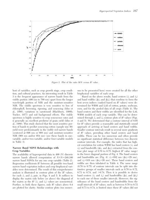
Hyperspectral Vegetation Indices 167Figure 3. Plot of the ratio M/N versus R 2 value.host of variables, such as crop growth stage, crop condi- ous to be presented here) were created for all the othertion, and cultural practices. An interesting result in Table biophysical variables of each crop.3 is the frequent appearance of narrow bands from the Based on the above results, band centers (k 1 and k 2 )visible portion (400 nm to 700 nm) apart from the longer and band widths (k 1 and k 2 ) that combine to form thewavelength portion of NIR and the moisture-sensitive best seven indices (ranked based on R 2 values) were determinedNIR. The visible spectrum is very sensitive to loss offor WBM and LAI of cotton, potato, soybeans,chlorophyll, browning, ripening, and senescing (Idso et corn, and for the pooled data of all crops (Table 4). Theal., 1980), variations in carotenoid (Blackburn, 1998b; band centers and their widths are identified for the LAI,Tucker, 1977) and soil background effects. The visible WBM models of each crop variable. This can be determinedspectrum is highly sensitive to crop senescence rates andthrough k 1 and k 2 contour plots of R 2 values (Figs.is generally an excellent predictor of grain yield (Idso et 4 and 5). We determined that a contour interval of 0.05al., 1980). This study showed that the most sensitive portionfor R 2 values provide a reasonable and statistically soundof bands to predict senescing cotton (sample size 50) approach of arriving at band centers and band widths.yield were predominantly in the visible red narrow bands Smaller contour intervals result in several more gradients(centered at 696 nm or 668 nm) and moisture-sensitive of R 2 values, providing other band centers and bandNIR (968 nm and/or 954 nm) (see these bands in one- widths. These can be too numerous and often providevariable, and/or two-variable, and/or four-variable models no significant statistical difference between two discretein Table 3).contour intervals. For example, the index that has highestcorrelation for cotton WBM has band centers (k 1 andNarrow Band NDVI Relationships withk 2 ) and bandwidth (k 1, and k 2 ) extracted from the con-Crop Variables tour plot range of 0.70 to 0.75 (highest R 2 value range)The availability of hyperspectral data in 490 (N) discrete in the lower diagonal portion of Fig. 4. The band centersnarrow bands allowed computation of NN240,100 and bandwidths are (Fig. 4): k 1 682 nm (k 1 28 nm),narrow band NDVIs for any one crop variable (Table 2). and k 2 918 nm (k 2 20 nm). These band centers andRegression coefficients R 2 between all possible two-band widths are then tabulated in Table 4. The same rangenarrow band vegetation indices and crop biophysical varitinctive(0.70 to 0.75) of contour intervals can be split into dis-ables were determined. The result of this comprehensivegroups of smaller intervals such as 0.70 to 0.72,analysis is illustrated in contour plots of the R 2 values, 0.73 to 0.74, and 0.74. Then it is possible to derivefor each k 1 and k 2 pair, in Figs. 4 and 5. It suffices to band centers (k 1 and k 2 ) and bandwidths (k 1 and k 2 )display the matrix only below (or above) the diagonal of to each one of these smaller intervals. However, the sig-the matrix as the R 2 (k 1 and k 2 ) values are symmetrical. nificance of the band centers and bandwidths from theFurther, in both these figures, only R 2 values above 0.4 small intervals of R 2 values, such as between 0.70 to 0.72are plotted for clarity. Similar contour plots (too numer- and 0.73 to 0.74, is limited since these R 2 values did not