Algebraic development of many-body perturbation theory in ...

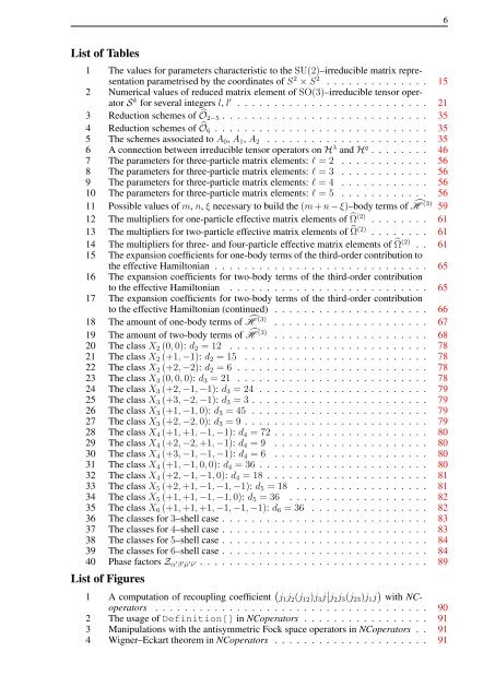
6List of Tables1 The values for parameters characteristic to the SU(2)–irreducible matrix representationparametrised by the coordinates of S 2 × S 2 . . . . . . . . . . . . . . 152 Numerical values of reduced matrix element of SO(3)–irreducible tensor operatorS k for several integers l, l ′ . . . . . . . . . . . . . . . . . . . . . . . . . . 213 Reduction schemes of Ô2−5 . . . . . . . . . . . . . . . . . . . . . . . . . . . . 354 Reduction schemes of Ô6 . . . . . . . . . . . . . . . . . . . . . . . . . . . . . 355 The schemes associated to A 0 , A 1 , A 2 . . . . . . . . . . . . . . . . . . . . . . 356 A connection between irreducible tensor operators on H λ and H q . . . . . . . . 467 The parameters for three-particle matrix elements: l = 2 . . . . . . . . . . . . 568 The parameters for three-particle matrix elements: l = 3 . . . . . . . . . . . . 569 The parameters for three-particle matrix elements: l = 4 . . . . . . . . . . . . 5610 The parameters for three-particle matrix elements: l = 5 . . . . . . . . . . . . 5611 Possible values of m, n, ξ necessary to build the (m + n − ξ)–body terms of Ĥ (3) 5912 The multipliers for one-particle effective matrix elements of ̂Ω (2) . . . . . . . . 6113 The multipliers for two-particle effective matrix elements of ̂Ω (2) . . . . . . . . 6114 The multipliers for three- and four-particle effective matrix elements of ̂Ω (2) . . 6115 The expansion coefficients for one-body terms of the third-order contribution tothe effective Hamiltonian . . . . . . . . . . . . . . . . . . . . . . . . . . . . . 6516 The expansion coefficients for two-body terms of the third-order contributionto the effective Hamiltonian . . . . . . . . . . . . . . . . . . . . . . . . . . . 6517 The expansion coefficients for two-body terms of the third-order contributionto the effective Hamiltonian (continued) . . . . . . . . . . . . . . . . . . . . . 6618 The amount of one-body terms of Ĥ (3) . . . . . . . . . . . . . . . . . . . . . 6719 The amount of two-body terms of Ĥ (3) . . . . . . . . . . . . . . . . . . . . . 6820 The class X 2 (0, 0): d 2 = 12 . . . . . . . . . . . . . . . . . . . . . . . . . . . 7821 The class X 2 (+1, −1): d 2 = 15 . . . . . . . . . . . . . . . . . . . . . . . . . 7822 The class X 2 (+2, −2): d 2 = 6 . . . . . . . . . . . . . . . . . . . . . . . . . . 7823 The class X 3 (0, 0, 0): d 3 = 21 . . . . . . . . . . . . . . . . . . . . . . . . . . 7824 The class X 3 (+2, −1, −1): d 3 = 24 . . . . . . . . . . . . . . . . . . . . . . . 7925 The class X 3 (+3, −2, −1): d 3 = 3 . . . . . . . . . . . . . . . . . . . . . . . . 7926 The class X 3 (+1, −1, 0): d 3 = 45 . . . . . . . . . . . . . . . . . . . . . . . . 7927 The class X 3 (+2, −2, 0): d 3 = 9 . . . . . . . . . . . . . . . . . . . . . . . . . 7928 The class X 4 (+1, +1, −1, −1): d 4 = 72 . . . . . . . . . . . . . . . . . . . . . 8029 The class X 4 (+2, −2, +1, −1): d 4 = 9 . . . . . . . . . . . . . . . . . . . . . 8030 The class X 4 (+3, −1, −1, −1): d 4 = 6 . . . . . . . . . . . . . . . . . . . . . 8031 The class X 4 (+1, −1, 0, 0): d 4 = 36 . . . . . . . . . . . . . . . . . . . . . . . 8032 The class X 4 (+2, −1, −1, 0): d 4 = 18 . . . . . . . . . . . . . . . . . . . . . . 8133 The class X 5 (+2, +1, −1, −1, −1): d 5 = 18 . . . . . . . . . . . . . . . . . . 8134 The class X 5 (+1, +1, −1, −1, 0): d 5 = 36 . . . . . . . . . . . . . . . . . . . 8235 The class X 6 (+1, +1, +1, −1, −1, −1): d 6 = 36 . . . . . . . . . . . . . . . . 8236 The classes for 3–shell case . . . . . . . . . . . . . . . . . . . . . . . . . . . . 8337 The classes for 4–shell case . . . . . . . . . . . . . . . . . . . . . . . . . . . . 8338 The classes for 5–shell case . . . . . . . . . . . . . . . . . . . . . . . . . . . . 8439 The classes for 6–shell case . . . . . . . . . . . . . . . . . . . . . . . . . . . . 8440 Phase factors Z α ′ β ′ ¯µ ′¯ν ′ . . . . . . . . . . . . . . . . . . . . . . . . . . . . . . . 89List of Figures1 A computation of recoupling coefficient ( j 1 j 2 (j 12 )j 3 j ∣ ∣j 2 j 3 (j 23 )j 1 j ) with NCoperators. . . . . . . . . . . . . . . . . . . . . . . . . . . . . . . . . . . . . 902 The usage of Definition[] in NCoperators . . . . . . . . . . . . . . . . . 913 Manipulations with the antisymmetric Fock space operators in NCoperators . . 914 Wigner–Eckart theorem in NCoperators . . . . . . . . . . . . . . . . . . . . . 91