Algebraic development of many-body perturbation theory in ...

More documents

Recommendations

Info

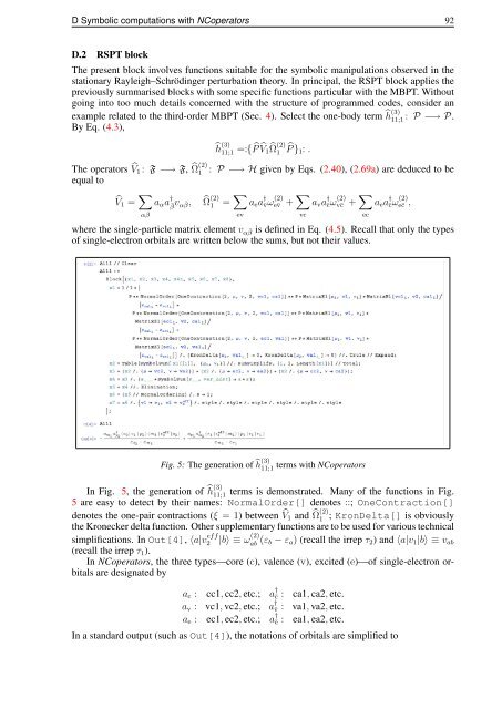
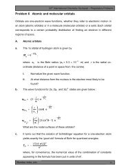
D Symbolic computations with NCoperators 92D.2 RSPT blockThe present block involves functions suitable for the symbolic manipulations observed in thestationary Rayleigh–Schrödinger perturbation theory. In principal, the RSPT block applies thepreviously summarised blocks with some specific functions particular with the MBPT. Withoutgoing into too much details concerned with the structure of programmed codes, consider anexample related to the third-order MBPT (Sec. 4). Select the one-body term ĥ(3) 11;1 : P −→ P.By Eq. (4.3),The operators ̂V 1 : F −→ F,equal toĥ (3)11;1 =:{ ̂P ̂V 1̂Ω(2) 1̂P } 1 : .̂Ω(2)1 : P −→ H given by Eqs. (2.40), (2.69a) are deduced to bêV 1 = ∑ αβa α a †¯βv α ¯β,̂Ω(2) 1 = ∑ ev(2)a e a†¯vω e¯v + ∑ vc(2)a v a†¯cω v¯c + ∑ ec(2)a e a†¯cω e¯c ,where the single-particle matrix element v α ¯β is defined in Eq. (4.5). Recall that only the typesof single-electron orbitals are written below the sums, but not their values.Fig. 5: The generation of ĥ(3) 11;1 terms with NCoperatorsIn Fig. 5, the generation of ĥ(3) 11;1 terms is demonstrated. Many of the functions in Fig.5 are easy to detect by their names: NormalOrder[] denotes ::; OneContraction[]denotes the one-pair contractions (ξ = 1) between ̂V (2)1 and ̂Ω 1 ; KronDelta[] is obviouslythe Kronecker delta function. Other supplementary functions are to be used for various technicalsimplifications. In Out[4], 〈a|v eff2 |b〉 ≡ ω (2)ab (ε b − ε a ) (recall the irrep τ 2 ) and 〈a|v 1 |b〉 ≡ v ab(recall the irrep τ 1 ).In NCoperators, the three types—core (c), valence (v), excited (e)—of single-electron orbitalsare designated bya c : cc1, cc2, etc.; a †¯c : ca1, ca2, etc.a v : vc1, vc2, etc.; a †¯v : va1, va2, etc.a e : ec1, ec2, etc.; a † ē : ea1, ea2, etc.In a standard output (such as Out[4]), the notations of orbitals are simplified to
D Symbolic computations with NCoperators 93c : a 1 , b 1 , c 1 , d 1 , e 1 , f 1 ¯c : a 2 , b 2 , c 2 , d 2 , e 2 , f 2v : m 1 , n 1 , p 1 , q 1 , k 1 , l 1 ¯v : m 2 , n 2 , p 2 , q 2 , k 2 , l 2e : r 1 , s 1 , t 1 , u 1 , w 1 , x 1 ē : r 2 , s 2 , t 2 , u 2 , w 2 , x 2Therefore, in accordance with Fig. 5, the generated terms ĥ(3) 11;1 areĥ (3)11;1 = ∑ eva v a †¯vv ve ω (2)e¯v− ∑ cva v a †¯vv c¯v ω (2)vc .(D.1)The next step is to restrict the model space P to its irreducible subspaces P Λ , that is, to expandĥ (3)11;1 into the sum of irreducible tensor operators W Λ (λ v˜λ¯v ). Refer to Eqs. (4.4), (4.17a).Consider the operators ĥ(3)+ 11;1 associated to ω (2)+α ¯β . In this case, it is easily done by using theexpression for SU(2)–invariant in the first row of Tab. 12: simply replace f(τ 2 λ µ λ ¯β)/(ε ¯β − ε µ )with Ω (2)+ (Λ) (recall Remark 4.1.1). But the present invariant has been obtained also makingµ ¯βuse of NCoperators. Thus, for the sake of clarity, the full procedure of angular reduction willbe demonstrated. This is, however, easy to perform.In Eq. (D.1), the first term contains the product of type ∑ µ v αµω (2)+ , while the second one –µ ¯βthe product of type ∑ µ v (2)+µ ¯βω αµ . These products determine the single-particle effective matrixelements. Then∑e∑cv ve ω (2)+e¯v = ∑ λ em e(−1) λe+me f(τ 1 λ v λ e )〈λ v m v λ e − m e |τ 1 m 1 〉× (−1) λ¯v+m¯v ∑ΛΩ (2)+e¯v (Λ)〈λ e m e λ¯v − m¯v |ΛM〉,v c¯v ω (2)+vc = ∑ λ cm c(−1) λ¯v+m¯v f(τ 1 λ c λ¯v )〈λ c m c λ¯v − m¯v |τ 1 m 1 〉× (−1) λc+mc ∑ΛΩ (2)+vc (Λ)〈λ v m v λ c − m c |ΛM〉.Finally, recalling that a v a †¯v = (−1) ∑ λ¯v+m¯v Λ W M Λ (λ v˜λ¯v )〈λ v m v λ¯v − m¯v |ΛM〉, the expressionin the first row of Tab. 15 (the case m = n = ξ = 1) is obtained by using the result in Fig. 1.A much more complicated task is to find Ω (2)+ (Λ). To generate the single-particle effectiveα ¯βmatrix elements ω (2) , make use of the generalised Bloch equation in Eq. (4.2). It follows thatα ¯βω (2) is the sum of ω(2)α ¯β ij;i+j−1 (α ¯β) ∀i, j = 1, 2, where the coefficients ω (2)ij;i+j−1 (α ¯β) are obtainedfrom the terms:{ ̂R̂V îΩ(1) ĵP −̂R̂Ω(1)ĵP ̂V i ̂P }i+j−1 : .The operator ̂R—also known as the resolvent [34]—is defined here by the action on somefunctional F (x † f 1, x † f 2, . . . , x † f a, x i1 , x i2 , . . . , x ia ) on H so that̂RF (x † f 1, x † f 2, . . . , x † f a, x ¯f1 , x ¯f2 , . . . , x ¯fa ) = [ D a (f ¯f) ] −1 ̂QF (x†f 1, x † f 2, . . . , x † f a, x ¯f1 , x ¯f2 , . . . , x ¯fa ).The energy denominator D a (f ¯f) is found from Eq. (2.65); the vectors x ¯fk (x † f k) ∀k = 1, 2, . . . , aof the single-particle Hilbert space are identified to be the single-particle eigenstates | ¯f k 〉 (〈f k |).The example how to generate the ω (2)11;1 terms is demonstrated in Figs. 6-7: in Fig. 6, thêR̂V 1̂Ω(1) 1̂R̂Ω(1)1terms { ̂P } 1 are generated, while in Fig. 7, the terms {result, ω (2)11;1 contains 9 expansion termsω 11;1(α (2) ¯β)(ε ¯β − ε α ) = ∑ v αµ ω (1)µ ¯β − ∑v ν ¯βω αν (1) ,µ(αβ)ν(αβ)̂P ̂V 1 ̂P }1 are derived. As a
Page 1 and 2:
INSTITUTE OF THEORETICAL PHYSICS AN
Page 3 and 4:
VILNIAUS UNIVERSITETOTEORINĖS FIZI
Page 5 and 6:
5Contents1 Introduction . . . . . .
Page 7 and 8:
75 The generation of ĥ(3) 11;1 ter
Page 9 and 10:
1 Introduction 9lation, the multi-c
Page 11 and 12:
1 Introduction 111.3 The scientific
Page 13 and 14:
2 Partitioning of function space an
Page 15 and 16:
Page 17 and 18:
Page 19 and 20:
Page 21 and 22:
Page 23 and 24:
Page 25:
Page 28 and 29:
Page 30 and 31:
Page 32 and 33:
Page 34 and 35:
3 Irreducible tensor operator techn
Page 36 and 37:
Page 38 and 39:
Page 40 and 41:
Page 42 and 43: 3 Irreducible tensor operator techn
Page 59 and 60: 4 Applications to the third-order M
Page 71 and 72: 5 Prime results and conclusions 71A
Page 73 and 74: A Basis coefficients 73(α1 α 2 (
Page 79 and 80: B The classification of three-parti
Page 85 and 86: C SU(2)-invariant part of the secon
Page 87 and 88: C SU(2)-invariant part of the secon
Page 89 and 90: D Symbolic computations with NCoper
Page 91: D Symbolic computations with NCoper
Page 101: D Symbolic computations with NCoper
show all

Algebraic development of many-body perturbation theory in ...

You also want an ePaper? Increase the reach of your titles

Delete template?

Save as template?