Scale transitions in solid mechanics based on computational ... - Cism

More documents

Recommendations

Info

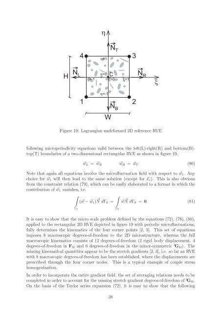
Figure 19: Lagrangian undeformed 2D reference RVEfollow<strong>in</strong>g microperiodicity equations valid between the left(L)-right(R) and bottom(B)-top(T) boundaries of a two-dimensional rectangular RVE as shown <strong>in</strong> figure 19.⃗w L = ⃗w R ⃗w B = ⃗w T (80)Note that aga<strong>in</strong> all equations <strong>in</strong>volve the microfluctuation field with respect to ⃗w 1 . Anychoice for ⃗w 1 will then lead to the same solution (except for ⃗x c ). This is also obviousfrom the constra<strong>in</strong>t relation (79), which can be easily elaborated to a format <strong>in</strong> which thecontribution of ⃗w 1 vanishes, i.e.∫∫(⃗w − ⃗w 1 ) NdΓ ⃗ 0 = ⃗w NdΓ ⃗ 0 = 0 (81)Γ 0 Γ 0It is easy to show that the micro scale problem def<strong>in</strong>ed by the equations (72), (78), (80),applied to the rectangular 2D RVE depicted <strong>in</strong> figure 19 with periodic microfluctuations,fully determ<strong>in</strong>es the k<strong>in</strong>ematics of the four corner po<strong>in</strong>ts [2, 3]. This set of equationsimposes 8 macroscopic degrees-of-freedom to the 2D microstructure, whereas the fullmacroscopic k<strong>in</strong>ematics consists of 12 degrees-of-freedom (2 rigid body displacement, 4degrees-of-freedom <strong>in</strong> F M and 6 degrees-of-freedom <strong>in</strong> the m<strong>in</strong>or-symmetric 3 G M ). Themiss<strong>in</strong>g k<strong>in</strong>ematical quantities appear to be the stretch gradients [2, 3], i.e. so far an RVEwith 8 macroscopic degrees-of-freedom has been established, where the displacements areprescribed through the four corner nodes. This is a typical example of couple stresshomogenization.In order to <strong>in</strong>corporate the entire gradient field, the set of averag<strong>in</strong>g relations needs to becompleted <strong>in</strong> order to account for the miss<strong>in</strong>g stretch gradient degrees-of-freedom of 3 G M .On the basis of the Taylor series expansion (72), it is easy to show that the follow<strong>in</strong>g38
averag<strong>in</strong>g theorem can be derived (by means of some manipulations of the equationsgiven <strong>in</strong> [3]), relat<strong>in</strong>g 3 G M to the position vectors ⃗x (implicitly <strong>in</strong>corporat<strong>in</strong>g the f<strong>in</strong>e scalecontribution through (74)) of all material po<strong>in</strong>ts <strong>in</strong> the the square RVE with <strong>in</strong>itial sizeW and volume V 0 :W 212[3 G M + 1 2( ) ]II : 3 G RT RTM +(I⃗c) RT = 1 ∫2V 0(⃗∇0,m (⃗x X)+[ ⃗ ∇ ⃗ 0,m (⃗x ⃗ )X)] T dV 0 (82)V 0In here, I is the second-order unit tensor, and RT stands for the right transpose, i.e.TijkRT = T ikj <strong>in</strong> <strong>in</strong>dex notation. The third term <strong>in</strong> the left-hand side of this equation ispresent to account for the deformed position ⃗x c of the center of the undeformed RVE,which is generally no longer the center of the deformed RVE. Comput<strong>in</strong>g the <strong>in</strong>tegral <strong>in</strong>the right-hand side of the latter equation through substitution of equation (74), reveals∫1(⃗∇0,m (⃗x X)+[2V ⃗ ∇ ⃗ 0,m (⃗x ⃗ )X)] T dV 0 =0V 0W 23 G M + W 212 24( )II : 3 G RT RTM +[I⃗c] RT + 1 ∫2V 0Γ 0(⃗X(⃗w − ⃗w1 ) N ⃗ + N(⃗w ⃗ − ⃗w 1 ) X ⃗ )dΓ 0(83)Enforc<strong>in</strong>g the averag<strong>in</strong>g relation (82) requires that the last <strong>in</strong>tegral <strong>in</strong> (83) should vanish,which leads to a new constra<strong>in</strong>t on the microfluctuation field.∫ (⃗X(⃗w − ⃗w1 ) N ⃗ + N(⃗w ⃗ − ⃗w 1 ) X ⃗ )dΓ 0 = 3 0 (84)Γ 0This boundary <strong>in</strong>tegral clearly <strong>in</strong>corporates (⃗w− ⃗w 1 ), which constra<strong>in</strong>s the position vectors⃗x of the boundary po<strong>in</strong>ts through (74). The microfluctuation ⃗w 1 (<strong>in</strong> the fixed boundarypo<strong>in</strong>t) cannot be elim<strong>in</strong>ated <strong>in</strong> general as done <strong>in</strong> the previously <strong>in</strong>troduced boundary<strong>in</strong>tegral (81). If constra<strong>in</strong>t (84) is enforced, it is easy to rewrite the averag<strong>in</strong>g equation (82)as a boundary <strong>in</strong>tegral( ) 3 G M + 1 2 II : 3 G RT RT 12M +W 2 [I⃗c]RT = 6 ∫ ( )⃗X⃗x N ⃗ + N⃗x ⃗ X ⃗ dΓV 0 W 2 0 (85)Γ 0Equation (85) typically illustrates that 3 G M is imposed on the RVE boundary, which isnecessary to construct a classical boundary value problem at the micro scale.For an <strong>in</strong>itially square RVE (H = W <strong>in</strong> figure 19), on which the microperiodicity equations(80) for the microfluctuation field hold, the constra<strong>in</strong>t (84) can be simplified to∫(⃗w L − ⃗w 1 )dΓ 0 = ⃗0Γ∫0L(86)(⃗w B − ⃗w 1 )dΓ 0 = ⃗0Γ 0BClearly, these two conditions enforce the shape of a part of the boundary to be equal<strong>in</strong> average to the shape ensu<strong>in</strong>g from the macroscopic field. Prescrib<strong>in</strong>g (86) at the39
Page 1 and 2: Scale tran
Page 3 and 4: 1 Introduction1.1 Mechanics across
Page 5 and 6: assumptions on the fin</str
Page 7 and 8: Figure 1: Macroscopic conti
Page 9 and 10: enization technique defin</
Page 11 and 12: local equilibrium and compatibility
Page 13 and 14: 3.4 Micro-scale RVE boundary condit
Page 15 and 16: where the relation (with account fo
Page 17 and 18: The volume average of the microscop
Page 19 and 20: whereby⃗u p =(F M − I)· ⃗X p
Page 21 and 22: Each constraint re
Page 23 and 24: Next, system (60) is further split,
Page 25 and 26: which allows to obtain</str
Page 27 and 28: (a)(b)Figure 7: Microstructural cel
Page 29 and 30: leads to much smaller RVE sizes tha
Page 31 and 32: (a)(b)Figure 11: Unit cell with one
Page 33 and 34: 100908070Axial stress, MPa605040302
Page 35 and 36: tensile test with the same material
Page 37: 8.2 Two-scale higher-order k<strong
Page 41 and 42: Elaboration of this equation leads
Page 43 and 44: where the fourth-order tensor 4 C (
Page 45: in figure 21. The

Scale transitions in solid mechanics based on computational ... - Cism

You also want an ePaper? Increase the reach of your titles

Delete template?

Save as template?