Sum-of-Squares Applications in Nonlinear Controller Synthesis

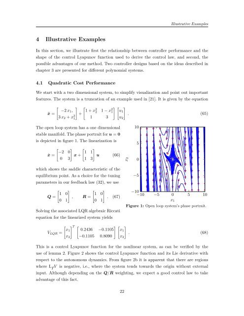
Illustrative Examples4 Illustrative ExamplesIn this section, we illustrate first the relationship between controller performance and theshape of the control Lyapunov function used to derive the control law, and second, thepossible advantages of our method. Two controller designs based on the ideas described inchapter 3 are presented for different polynomial systems.4.1 Quadratic Cost PerformanceWe start with a two dimensional system, to simplify visualization and point out importantfeatures. The system is a truncation of an example used in [21]. It is given by the equation[ ] [−2 x1 , 1 + x2ẋ =3 x 2 + x 3 + 2 1 − x 2 ] [ ]1 u1. (65)1 1 3 u 2The open loop system has a one dimensionalstable manifold. The phase portrait for u = 0is depicted in figure 1. The linearization is[ ] [ ]−2 0 1 1ẋ = x + u (66)0 3 1 3x21050which shows the saddle characteristic of theequilibrium point. As a choice for the tuningparameters in our feedback law (32), we use[ ][ ]1 01 0Q = , R = . (67)0 10 1Solving the associated LQR algebraic Riccatiequation for the linearized system yields−5−10−10 −5 0 5 10x 1Figure 1: Open loop system’s phase portrait.V LQR =[ ] T [ ] [ ]x1 0.2436 −0.1105 x1x 2 −0.1105 0.8090 x 2. (68)This is a control Lyapunov function for the nonlinear system, as can be verified by theuse of lemma 2. Figure 2 shows the control Lyapunov function and its Lie derivative withrespect to the autonomous dynamics. From figure 2b it is apparent that there are regionswhere L f V is negative, i.e., where the system tends towards the origin without externalinput. Although depending on the Q/R weighting, we expect a good control law to takeadvantage of this fact.22