r |f(z) - Christian-Albrechts-Universität zu Kiel

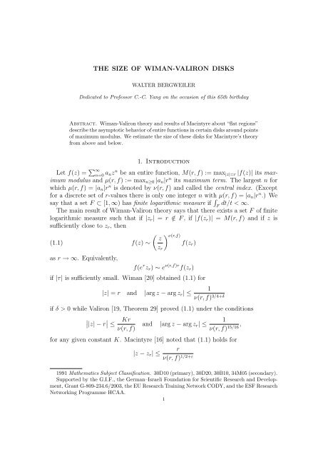
THE SIZE OF WIMAN-VALIRON DISKSWALTER BERGWEILERDedicated to Professor C.-C. Yang on the occasion of this 65th birthdayAbstract. Wiman-Valiron theory and results of Macintyre about “flat regions”describe the asymptotic behavior of entire functions in certain disks around pointsof maximum modulus. We estimate the size of these disks for Macintyre’s theoryfrom above and below.1. IntroductionLet f(z) = ∑ ∞n=0 a nz n be an entire function, M(r, f) := max |z|=r |f(z)| its maximummodulus and µ(r, f) := max n≥0 |a n |r n its maximum term. The largest n forwhich µ(r, f) = |a n |r n is denoted by ν(r, f) and called the central index. (Exceptfor a discrete set of r-values there is only one integer n with µ(r, f) = |a n |r n .) Wesay that a set F ⊂ [1, ∞) has finite logarithmic measure if ∫ dt/t < ∞.FThe main result of Wiman-Valiron theory says that there exists a set F of finitelogarithmic measure such that if |z r | = r /∈ F , if |f(z r )| = M(r, f) and if z issufficiently close to z r , then(1.1) f(z) ∼( zz r) ν(r,f)f(z r )as r → ∞. Equivalently,f(e τ z r ) ∼ e ν(r,f)τ f(z r )if |τ| is sufficiently small. Wiman [20] obtained (1.1) for|z| = r and |arg z − arg z r | ≤1ν(r, f) 3/4+δif δ > 0 while Valiron [19, Theorem 29] proved (1.1) under the conditions∣∣|z| − r ∣ ∣ ≤Krν(r, f)and|arg z − arg z r | ≤1ν(r, f) 15/16 ,for any given constant K. Macintyre [16] noted that (1.1) holds forr|z − z r | ≤ν(r, f) 1/2+ε1991 Mathematics Subject Classification. 30D10 (primary), 30D20, 30B10, 34M05 (secondary).Supported by the G.I.F., the German–Israeli Foundation for Scientific Research and Development,Grant G-809-234.6/2003, the EU Research Training Network CODY, and the ESF ResearchNetworking Programme HCAA.1

2 WALTER BERGWEILERif ε > 0. The sharpest estimates are due to Hayman [10] whose results imply thatifψ(t) = t · log t · log log t · . . . · log m−1 t · (log m t) 1+ε ,where ε > 0, m ∈ N and log m denotes the m-th iterate of the logarithm, then (1.1)holds forr|z − z r | ≤ √ .ψ(ν(r, f)) log ψ(ν(r, f))Results similar to those of Wiman-Valiron theory were obtained by Macintyre [16]with ν(r, f) replaced byd log M(r, f)a(r, f) := .d log rRecall here that log M(r, f) is convex in log r. Since convex functions have nondecreasingleft and right derivatives and since they are differentiable except foran at most countable set, the derivative of log M(r, f) with respect to log r existsexcept possibly for a countable set of r-values. (Actually, by a result of Blumenthal(see [19, Section II.3]), the set of r-values where log M(r, f) is not differentiableis discrete.) To be definite, we shall always denote by a(r, f) the right derivativeof log M(r, f) with respect to log r. Then a(r, f) is nondecreasing and it can beshown thata(r, f) = z rf ′ (z r )f(z r )except for an at most countable set of r-values. The result of Macintyre [16,Theorem 3] says thatfor(1.2) |z − z r | ≤f(z) ∼( zz r) a(r,f)f(z r )r(log M(r, f)) 1/2+εas r → ∞, r /∈ F .More recently, a result of this type was obtained in [2]. There it is not requiredthat f is entire but only that f is as in the following definition.Definition 1.1. Let D be an unbounded domain in C whose boundary consists ofpiecewise smooth curves. Suppose that the complement of D is unbounded. Letf be a complex-valued function whose domain of definition contains the closure Dof D. Then D is called a direct tract of f if f is holomorphic in D and continuousin D and if there exists R > 0 such that |f(z)| = R for z ∈ ∂D while |f(z)| > Rfor z ∈ D.We note that every transcendental entire function has a direct tract. Let f, D, Rbe as in the above definition and putM(r, f, D) :=max |f(z)|.|z|=r,z∈D

WIMAN-VALIRON DISKS 3Then log M(r, f, D) is again convex in log r. Denoting by a(r, f, D) the right derivativeof log M(r, f, D) with respect to log r we see as before that a(r, f, D) isnondecreasing anda(r, f, D) = z rf ′ (z r )f(z r )except for an at most countable set of r-values, with z r ∈ D such that |z r | = r and|f(z r )| = M(r, f, D). It follows from a result of Fuchs [7] thatlog M(r, f, D)limr→∞ log r= ∞ and limr→∞a(r, f, D) = ∞.The main result of [2] says that if τ > 1 , then there exists a set F of finite2logarithmic measure such that(1.3) f(z) ∼( zz r) a(r,f,D)f(z r )for(1.4) |z − z r | 0 and m ∈ N. Here (1.5) holds for α > 1 while (1.6) holds for α ≤ 1.For these functions we have1 ≤ tψ′ (t)ψ(t) ≤ 1 + o(1)as t → ∞. Therefore it does not seem to be a severe restriction to impose thecondition that ψ is differentiable and satisfies(1.7) K ≤ tψ′ (t)ψ(t) ≤ Lfor certain constants K and L satisfying 0 ≤ K ≤ 1 < L.

4 WALTER BERGWEILEROur results are as follows.Theorem 1.1. Let t 0 > 0 and let ψ : [t 0 , ∞) → (0, ∞) be a differentiable functionsatisfying (1.5) and (1.7) for some K > 0 and L < 2.Let f be a function with a direct tract D and let z r ∈ D with |z r | = r and|f(z r )| = M(r, f, D). Then there exists a set F of finite logarithmic measure suchthat(1.8) f(z) ∼( zz r) a(r,f,D)f(z r ) for |z − z r | ≤as r → ∞, r /∈ F .r√ψ(a(r, f, D))Theorem 1.2. Let t 0 > 0 and let ψ : [t 0 , ∞) → (0, ∞) be a differentiable functionsatisfying (1.6) and (1.7) for K = 1 and some L < 6 5 .Then there exists an entire function f which has exactly one tract D such that ifr is sufficiently large and |z| = r, then the disk of radius r/ √ ψ(a(r, f, D)) aroundz contains a zero of f.In particular it follows under the hypotheses of Theorem 1.2 that the disk mentionedis not contained in D and that (1.8) does not hold.Remark 1. Our method also yields that if f is entire and z r is a point of modulus rwith |f(z r )| = M(r, f), then (1.8) holds with a(r, f, D) replaced by a(r, f). Herewe only note that if D r is the direct tract containing z r , thena(r, f) = a(r, f, D r ) = z rf ′ (z r )f(z r )except for an at most countable set of r-values.We also note that if ψ satisfies (1.5), then(1.9) a(r, f, D) ≤ ψ(log M(r, f, D))outside a set of finite logarithmic measure. In fact, if s 0 := log M(r 0 , f, D) ≥ t 0and if F denotes the set of all r ≥ r 0 where (1.9) does not hold, then∫Fdtt ≤ ∫F∫a(t, f, D) dt ∞∫ψ(log M(t, f, D)) t ≤ a(t, f, D) dt ∞r 0ψ(log M(t, f, D)) t = s 0dtψ(t) < ∞.We deduce that the condition |z − z r | ≤ r/ √ ψ(a(r, f, D)) in (1.8) can be replacedbyr|z − z r | ≤ √ .ψ(ψ(log M(r, f, D)))For entire f we can again replace M(r, f, D) by M(r, f) if |f(z r )| = M(r, f). Withψ(t) = t 1+δ we recover Macintyre’s condition (1.2).Remark 2. In the papers on Wiman-Valiron theory cited above it is usually notrequired that |f(z r )| = M(r, f) but only that |f(z r )| ≥ ηM(r, f) for some η ∈ (0, 1),possibly depending on r. It is then shown that (1.1) holds for z in some diskaround z r whose size depends on η. In [2] only the case η = 1 is considered,although the method allows to deal with the case 0 < η < 1 as well. For the sakeof simplicity we also restrict to the case η = 1 in this paper.

WIMAN-VALIRON DISKS 5Remark 3. It was shown in [1] that the estimate on the size of the exceptional set Fis best possible in Wiman-Valiron theory, and it follows from the results there thatthis also holds for Macintyre’s theory and Theorem 1.1.Remark 4. We do not discuss the numerous applications that the theories ofWiman-Valiron and Macintyre have found, but just mention some references withapplications to complex differential equations [6, 12, 13, 21], distribution of zerosof derivatives [4, 14], and complex dynamics [2, 5, 11].2. Proof of Theorem 1.1Let D be a direct tract of f. The proof in [2] that (1.3) holds for z satisfying (1.4)relies on a lemma [2, Lemma 11.3] which says that if β > 1 , then there exists a set2F of finite logarithmic measure such that(2.1) log M(s, f, D) ≤ log M(r, f, D) + a(r, f, D) log s r + o(1)for(2.2)∣∣log s ∣ ≤r1a(r, f, D) β ,uniformly as r → ∞, r /∈ F . In order to prove Theorem 1.1 we shall prove that ifψ satisfies the hypothesis of this theorem, then (2.2) can be replaced by∣(2.3)∣log s 1∣ ≤ √ .r ψ(a(r, f, D))In order to prove that (2.1) holds under the assumption (2.3) we use the followinglemma.Lemma 2.1. Let x 0 > 0 and let T : [x 0 , ∞) → (0, ∞) be nondecreasing. Lett 0 := T (x 0 ) and let σ 1 , σ 2 : [t 0 , ∞) → (0, ∞) be nondecreasing functions such that∫ ∞t 0dtσ 1 (t)σ 2 (t) < ∞.Suppose also that σ 2 is differentiable and satisfies0 ≤ tσ′ 2(t)σ 2 (t) ≤ 1 − δfor t ≥ t 0 and some δ > 0. Then there exists a set E ⊂ [x 0 , ∞) of finite measuresuch that if x /∈ E, then()1(2.4) T x +< T (x) + σ 2 (T (x))σ 1 (T (x))and(2.5) T()1x −> T (x) − σ 2 (T (x)).σ 1 (T (x))

6 WALTER BERGWEILERProof. First we note that x − 1/σ 1 (T (x)) ≥ x 0 for sufficiently large x, say x ≥ x ′ 0.Thus the left hand side of (2.5) is defined for x ≥ x ′ 0. Denoting by E 1 the subsetof [x 0 , ∞) where (2.4) fails and by E 2 the subset of [x ′ 0, ∞) where (2.5) fails we canthus take E = [x 0 , x ′ 0] ∪ E 1 ∪ E 2 .We put G(t) := t/σ 2 (t). Sincethe function G is increasing and henceG (t + σ 2 (t)) − G(t) =tG ′ (t)G(t) = 1 − tσ′ 2(t)σ 2 (t) ≥ δ≥≥∫ t+σ2 (t)δt∫ t+σ2 (t)tδG(t)= δG(t) logG ′ (u)duG(u)udu∫ t+σ2 (t)tduu(1 + 1 )G(t)for t ≥ t 0 . Since the function x ↦→ x log (1 + 1/x) is increasing for x > 0 we deducethat((2.6) G (t + σ 2 (t)) − G(t) ≥ η := δG(t 0 ) log 1 + 1 )> 0G(t 0 )for t ≥ t 0 . Similarly,(2.7)G(t) − G (t − σ 2 (t)) =≥∫ tδ= δ≥= δt−σ 2 (t)∫ tt−σ 2 (t)∫ tt−σ 2 (t)∫ t1δσ 2 (t)G ′ (u)duG(u)ududuσ 2 (u)t−σ 2 (t)for t ≥ t 0 .To estimate the size of E 1 we may assume that E 1 is unbounded. We choosex 1 ∈ E 1 ∩ [inf E 1 , inf E 1 + 1 2 ] and put x′ 1 := x 1 + 1/σ 1 (T (x 1 )). Recursively we thenchoosex j ∈ E 1 ∩ [ inf ( E 1 ∩ [x ′ j−1, ∞) ) , inf ( E 1 ∩ [x ′ j−1, ∞) ) + 2 −j]and put x ′ j := x j + 1/σ 1 (T (x j )). Then()T (x j+1 ) ≥ T (x ′ 1j) = T x j +≥ T (x j ) + σ 2 (T (x j ))σ 1 (T (x j ))du

WIMAN-VALIRON DISKS 7and henceG(T (x j+1 )) ≥ G (T (x j ) + σ 2 (T (x j ))) ≥ G (T (x j )) + ηby (2.6). Induction shows that(2.8) G(T (x j )) ≥ G (T (x 1 )) + (j − 1)ηfor j ∈ N. In particular it follows that x j → ∞ so thatE 1 ⊂∞⋃j=1[ ]xj − 2 −j , x ′ j .Hencemeas E 1 ≤∞∑ (x′j − x j + 2 −j) =j=1∞∑j=11σ 1 (T (x j )) + 1.With H := σ 1 ◦ G −1 and u 0 := G (T (x 1 )) we deduce from (2.8) thatHence∞∑j=2∞1σ 1 (T (x j )) ≤ ∑σ 1 (T (x j )) = H(G(T (x j ))) ≥ H(u 0 + (j − 1)η).j=21H(u 0 + (j − 1)η) ≤ 1 ∫ ∞η u 0duH(u) = 1 ∫ ∞G ′ (v)η T (x 1 ) σ 1 (v) dv.Sincewe obtainAltogether we have∞∑j=2G ′ (v) = 1σ 2 (v) − vσ′ 2(v)σ 2 (v) 2 ≤ 1σ 2 (v)1σ 1 (T (x j )) ≤ 1 ∫ ∞dvη T (x 1 ) σ 1 (v)σ 2 (v) < ∞.meas E 1 ≤ 1σ 1 (t 0 ) + 1 η∫ ∞t 0dvσ 1 (v)σ 2 (v) + 1 < ∞.To estimate E 2 we proceed similarly. We may assume that E 2 ≠ ∅ and fix R > x ′ 0so large that E 2 ∩ [x ′ 0, R] ≠ ∅. We choosez 1 ∈ E 2 ∩ [ sup (E 2 ∩ [x ′ 0, R]) − 1 2 , sup (E 2 ∩ [x ′ 0, R]) ]and put z ′ 1 := z 1 − 1/σ 1 (T (z 1 )). Recursively we then choosez j ∈ E 2 ∩ [ sup ( E 2 ∩ [x ′ 0, z ′ j−1] ) − 2 −j , sup ( E 2 ∩ [x ′ 0, z ′ j−1] )]

8 WALTER BERGWEILERand put z ′ j := z j − 1/σ 1 (T (z j )), as long as E 2 ∩ [x ′ 0, z ′ j−1] ≠ ∅. However, sinceT (z j+1 ) ≤ T (z j)′()1= T z j −σ 1 (T (z j ))≤ T (z j ) − σ 2 (T (z j ))()1= 1 −T (z j )≤≤(1 −(1 −G(T (z j )))1T (z j )G(T (z 1 ))) j1T (z 1 ),G(T (z 1 ))the process stops and we obtain two finite sequences (z 1 , . . . , z N ) and (z 1, ′ . . . , z N ′ )withN⋃E 2 ∩ [x ′ 0, R] ⊂ [z j, ′ z j + 2 −j ].With y j := z N−j+1 we thus haveandHenceby (2.7) and thusE 2 ∩ [x ′ 0, R] ⊂j=1N⋃[y j, ′ y j + 2 j−N−1 ]j=1T (y j ) ≤ T (y j+1 ) − σ 2 (T (y j+1 )).G(T (y j )) ≤ G (T (y j+1 ) − σ 2 (T (y j+1 ))) ≤ G (T (y j+1 )) − δG(T (y j )) ≥ G(T (y 1 )) + (j − 1)δby induction. Now the estimate for E 2 is very similar to that for E 1 . We obtainmeas (E 2 ∩ [x ′ 0, R])and hence meas E 2 < ∞.≤=≤≤N∑(y j − y j ′ + 2 j−N−1 )j=1N∑N1σ 1 (T (y j )) + ∑j=11σ 1 (T (y 1 )) + 1 δ1σ 1 (t 0 ) + 1 δ∫ ∞t 0j=1∫ ∞T (y 1 )2 j−N−1duH(u) + 1duσ 1 (u)σ 2 (u) + 1□

WIMAN-VALIRON DISKS 9Remark. Lemma 2.1 was proved in [2, Lemma 11.1] in the case that σ 1 (t) = t β andσ 2 (t) = t 1−α where 0 < α < β. The method of proof used here is similar, goingback to a classical lemma of Borel; see [3, §3.3], [8, p. 90] and [17].Similarly as in [2] we apply Lemma 2.1 to the (right) derivative Φ ′ of a convexfunction Φ.Lemma 2.2. Let x 0 > 0 and let Φ : [x 0 , ∞) → (0, ∞) be increasing and convex. Lett 0 := Φ(x 0 ) and let ψ : [t 0 , ∞) → (0, ∞) be a differentiable function satisfying (1.5)and (1.7) with K > 0 and L < 2. Then there exists a set E ⊂ [x 0 , ∞) of finitemeasure such that(2.9) Φ(x + h) ≤ Φ(x) + Φ ′ (x)h + o(1) for |h| ≤1√ , x /∈ E,ψ(Φ′ (x))uniformly as x → ∞.Proof. First we note that lim x→∞ Φ ′ (x) exists since Φ ′ is nondecreasing. It is easyto see that (2.9) holds without an exceptional set E if this limit is finite. Hence weassume that lim x→∞ Φ ′ (x) = ∞.LetV (t) :=∫ ∞tduψ(u)so that V ′ (t) = −1/ψ(t). We may assume that K < 1 and apply Lemma 2.1 withT = Φ ′ and(2.10) σ 1 (t) = σ 2 (t) = V (t) K/2√ ψ(t).To show that the hypotheses of this lemma are satisfied we note that∫ tt 0∫dutσ 1 (u)σ 2 (u) =t 0V (u) −Kdu = 1 (V (t0 ) 1−K − V (t) 1−K)ψ(u) 1 − Kand thus∫ ∞t 0duσ 1 (u)σ 2 (u) < ∞.We also have(2.11)tσ ′ 2(t)σ 2 (t) = K 2tV ′ (t)V (t) + 1 tψ ′ (t)2 ψ(t) .Since V ′ (t) = −1/ψ(t) < 0 this implies thattσ 2(t)′σ 2 (t) ≤ 1 tψ ′ (t)2 ψ(t) ≤ L 2 < 1.

10 WALTER BERGWEILEROn the other hand, since ψ is increasing it follows from (1.5) that ψ(t)/t → ∞ ast → ∞ and thus we find, using (1.7), thatIt follows that0 < −tV ′ (t)t=ψ(t)∫ ∞( uψ ′ (u)=t ψ(u) − 12 ψ(u)∫ ∞( uψ ′ (u)=t ψ(u)≤ (L − 1)V (t).tV ′ (t)V (t))du) duψ(u) − V (t)≥ −(L − 1)and this, together with (1.7) and (2.11), implies thattσ ′ 2(t)σ 2 (t) ≥ −K 2 (L − 1) + K 2Thus the hypotheses of Lemma 2.1 are satisfied.Next we note that (2.10) yields that(√ )σ k (t) = o ψ(t)=K(2 − L)2> 0.as t → ∞ for k ∈ {1, 2}. In particular, we find that σ k (t) ≤ √ ψ(t) for large t.Lemma 2.1 now yields that if x /∈ E is large and 0 < h ≤ 1/ √ ψ (Φ ′ (x)), thenΦ(x + h) = Φ(x) +∫ x+hxΦ ′ (u)du≤ Φ(x) + Φ ′ (x + h)h)≤ Φ(x) + Φ(x ′ 1+hσ 1 (Φ ′ (x))≤ Φ(x) + (Φ ′ (x) + σ 2 (Φ ′ (x))) h≤ Φ(x) + Φ ′ (x)h + σ 2 (Φ ′ (x))√ψ (Φ′ (x))and hence Φ(x) + Φ ′ (x)h + o(1) as x → ∞. The case −1/ √ ψ (Φ ′ (x)) ≤ h < 0 isanalogous.□Remark. If we apply Lemma 2.1 not to the functions defined by (2.10), as we did inthe above proof, but to the functions σ 1 (t) = σ 2 (t) = √ ψ(t), then we obtain (2.9)with o(1) replaced by 1. Choosing σ 1 (t) = σ 2 (t) = ε √ ψ(t) yields (2.9) with o(1)replaced by ε.

WIMAN-VALIRON DISKS 11We apply Lemma 2.2 to Φ(x) = log M(e x , f, D). Then Φ ′ (x) = a(e x , f, D). Withr = e x and s = e x+h we obtainlog M(s, f, D) = Φ(x + h)≤Φ(x) + Φ ′ (x)h + o(1)= log M(r, f, D) + a(r, f, D) log s r + o(1)for r /∈ F = exp E, provided that∣∣log s 1∣ = |h| ≤ √rψ(Φ′ (x)) = 1√ .ψ(a(r, f, D))This means that (2.1) holds for r /∈ F under the assumption (2.3).The deduction of Theorem 1.1 from the result that (2.1) holds for s satisfying(2.3) if r /∈ F is similar to the arguments in [2] where the validity of (2.1)under the stronger condition (2.2) is used to show that (1.3) holds for z satisfying(1.4).3. Proof of Theorem 1.23.1. Preliminaries. We first note that (1.6) and (1.7) also hold with ψ(x) replacedby αψ(βx) where α, β > 0, and thus it suffices to show that there exist γ, δ > 0 suchthat the disk of radius γr/ √ ψ(δa(r, f, D)) around z contains a zero of f if |z| = ris large. Moreover, we see that we may assume that ψ(t 0 ) ≥ t 0 ≥ 1.We define A 1 : [1, ∞) → [t 0 , ∞) by(3.1) log r =With φ : [t 0 , ∞) → [0, ∞),φ(t) :=∫ A1 (r)t 0∫ tt 0duψ(u) .duψ(u)we thus have A 1 (r) = φ −1 (log r). The function f constructed will satisfya(r, f) = a(r, f, D) ∼ A 1 (r)as r → ∞. However, before we can define the function f we will have to introducesome auxiliary functions and study their properties.We first note that it follows from (1.7) and the assumption that K = 1 thatUsing that ψ(t 0 ) ≥ t 0 we see thatlog tt 0≤ log ψ(t)ψ(t 0 ) ≤ L log tt 0.(3.2) t ≤ ψ(t) ≤ ct Lfor t ≥ t 0 and c := ψ(t 0 )t −L0 .

12 WALTER BERGWEILERIt follows from (3.1) that A 1 (r) is differentiable and A ′ 1(r) = ψ(A 1 (r))/r. Thisimplies that A 2 (r) := rA ′ 1(r) = ψ(A 1 (r)) is also differentiable so that we may defineA 3 (r) := rA ′ 2(r). The functions A 1 , A 2 and A 3 are thus related by(3.3) A 2 (r) = dA 1(r)d log r = rA′ 1(r) and A 3 (r) = dA 2(r)d log r = rA′ 2(r).Since ψ(t) ≥ t we have φ(t) ≤ log(t/t 0 ) and thus A 1 (r) ≥ t 0 r ≥ r for r ≥ 1.Using (3.2) and recalling that (1.7) holds with K = 1 we find that A 2 (r) ≥ A 1 (r)andA 3 (r) = rA ′ 2(r) = ψ ′ (A 1 (r))A 2 (r) ≥ ψ(A 1(r))A 2 (r) ≥ A 2 (r).A 1 (r)Putting together the last estimates we thus have(3.4) A 3 (r) ≥ A 2 (r) ≥ A 1 (r) ≥ r ≥ 1 > 0for r ≥ 1. Combining this with (3.3) we see that A 1 and A 2 are increasing andthat A 1 (r) is a convex function of log r. Moreover, (1.7) yields that(3.5) 1 ≤ A 1(r)ψ ′ (A 1 (r))ψ(A 1 (r))For ρ > 1 and r > 1 we thus haveChoosing1A 2 (r) − 1A 2 (ρr)=≤≤== A 1(r)A 3 (r)A 2 (r) 2 ≤ L.∫ ρr(3.6) ρ := 1 + A 1(r)2A 2 (r)we obtainand hence(3.7) A 2(rIt follows from (3.2) thatA 3 (s) dsr A 2 (s) 2 s∫ ρr1 dsLr A 1 (s) s∫L ρrdsA 1 (r) r sLlog ρ.A 1 (r)1 − A (2(r)A 2 (ρr) ≤ LA 2(r)A 1 (r) log 1 + A )1(r)≤ L 2A 2 (r) 2 ≤ 3 5(1 + A ))1(r)= A 2 (ρr) ≤ 5 2A 2 (r)2 A 2(r).(3.8) A 2 (r) = ψ(A 1 (r)) ≤ cA 1 (r) Lso that(3.9) A 1 (r) ≥ c −1/L A 2 (r) 1/L .

Together with (3.5) we deduce thatHenceA 0 (r) :=≥≥=∫ rWIMAN-VALIRON DISKS 13A 1 (s) dss1∫ r1 ( ) 2 A1 (s)A 3 (s) dsL 1 A 2 (s) s∫1 rALc 2/L 2 (s) 2/L−2 A 3 (s) ds1s(A2 (r) 2/L−1 − A 2 (1) 2/L−1) .1c 2/L (2 − L)(3.10) A 2 (r) = o ( A 0 (r) L/(2−L))as r → ∞. We also note that (3.5) yieldsso that(3.11)A 1 (r) 2A 2 (r)We now define g : [1, ∞) → [0, ∞),∫ r(= A 1 (s) 2 − A )1(s)A 3 (s) ds1A 2 (s) 2 s + A 1(1) 2A 2 (1)∫ r≥ (2 − L) A 1 (s) ds1 s= (2 − L)A 0 (r)A 0 (r)A 2 (r)A 1 (r) 2 ≤ 12 − L < 5 4 .g(r) :=∫ r1√A2 (s) dssso that g ′ (r) = √ A 2 (r)/r ≥ 1/ √ r > 0. Thus g is increasing and hence the inversefunction h := g −1 : [0, ∞) → [1, ∞) exists. We will have to use various estimatesinvolving the derivatives of h. First we note thatand hence(3.12)h ′ (t) =1g ′ (h(t)) =h(t)√A2 (h(t))h(t)h ′ (t) = √ A 2 (h(t)) ≥ 1for t ≥ 0 by (3.4). We deduce that( )d h(t)(3.13)= A′ 2(h(t))h ′ (t)dt h ′ (t) 2 √ A 2 (h(t)) = A 3(h(t))h ′ (t)2 √ A 2 (h(t))h(t) = A 3(h(t))2A 2 (h(t)) .Similarly we find that(h ′′ (t)h ′ (t) = 1 − A )3(h(t)) 1√2A 2 (h(t)) A2 (h(t))

14 WALTER BERGWEILERwhich together with (3.4), (3.5) and (3.8) yields thath ′′ (t)∣ h ′ (t) ∣ ≤ 3 A 3 (h(t))2 A 2 (h(t)) ≤ 3L √A2 (h(t))≤ 3L√ cA 3/2 1 (h(t)) L/2−1 = o(1)2 A 1 (h(t)) 2as t → ∞. It follows that if 0 ≤ s ≤ 1, thenand hencelog h′ (t + s)h ′ (t)=∫ t+sth ′′ (u)du = o(1)h ′ (u)(3.14) h ′ (t + s) ∼ h ′ (t) for 0 ≤ s ≤ 1as t → ∞. For later use we also note that (3.5), (3.13) and (3.9) yield that ifr > h(t), then ∣∣∣∣ (d h(t)dt h ′ (t) log r )∣ ∣∣∣ =A 3 (h(t))h(t) ∣2A 2 (h(t)) log r ∣ ∣∣∣h(t) − 1(3.15) ≤ L 2≤ Lc1/LA 2 (h(t))A 1 (h(t)) logrh(t) + 1≤2A 2 (h(t)) 1−1/L log r + 1Lc1/LA 2 (r) 1−1/L log r + 1.2Finally we shall need the following two lemmas.Lemma 3.1. Let R > 0 and let F : [0, R] → R be differentiable. Then[R]∑∫ RF (k) − F (t)dt∣R−[R] ∣ ≤ R sup |F ′ (t)|.0 0 such thatβ ′′ (x)β ′ (x) ≤ (x)Lβ′ β(x)for x ≥ x 0 . Suppose also that α(x) ∼ β(x) as x → ∞. Then α ′ (x) ∼ β ′ (x) asx → ∞.3.2. The maximum modulus of f. Let h be as in the previous section. Wedefine⎛∞∏( ) h i⎞h(k)zhf(z) := ⎝1 ′ (k)+⎠ .h(k)k=1Note that [h ′ (k)/h(k)] ≥ 1 for all k ∈ N by (3.12).

WIMAN-VALIRON DISKS 15It will be apparent from the computations below that the infinite product convergesabsolutely and locally uniformly and thus defines an entire function whichhas [h(k)/h ′ (k)] equally spaced zeros on the circle of radius h(k) around 0. In thissection we determine the asymptotic behavior of log M(r, f) and a(r, f) as r → ∞.In §3.3 we will then show that there exist γ, δ > 0 such that if |z| is sufficientlylarge, then the disk of radius γ|z|/ √ ψ(δa(|z|, f)) contains a zero of f. Finally wewill show in §3.4 that f has only one direct tract D so that a(r, f) = a(r, f, D),thereby completing the proof of Theorem 1.2.Let now r > 0, define ρ by (3.6) and putWithwe haveS 1 :=First we note thatS 1 ≤[g(r)]∑k=1[g(r)]∑k=1([ h(k)h ′ (k)⎛a k := log ⎝1 +a k , S 2 :=]log[g(ρr)]∑k=[g(r)]+1( r) h h(k)h ′ (k)h(k)i⎞⎠ .a k and S 3 :=log M(r, f) ≤ S 1 + S 2 + S 3 .r )h(k) + log 2 ≤and hence Lemma 3.1 and (3.15) yield thatS 1 ≤∫ g(r)0h(t)h ′ (t) logr ( Lc1/Lh(t) dt + g(r) 2Substitution and integration by parts yield∫ g(r)0h(t)h ′ (t) log r ∫ rh(t) dt =(3.16) =Moreover,(3.17) g(r) =∫ rCombining the above estimates we obtain1==1∫ r1∫ r1∫ r1⎛[g(r)]∑⎝k=1h(k)h ′ (k) log∞∑k=[g(ρr)]+1a k⎞r ⎠ + g(r) log 2h(k))A 2 (r) 1−1/L log r + 1 + g(r) log 2.sg ′ (s) 2 log r s dsA 2 (s)slog r s dsA ′ 1(s) log r s dsA 1 (s) dss − A 1(1) log r= A 0 (r) − t 0 log r.√A2 (s) dss ≤ √ A 2 (r) log r.S 1 ≤ A 0 (r) + O ( A 2 (r) 3/2−1/L (log r) 2)

16 WALTER BERGWEILERas r → ∞. Now (3.10) yields thatA 2 (r) 3/2−1/L = A 2 (r) (3L−2)/2L = o ( A 0 (r) (3L−2)/(4−2L))as r → ∞. Since L < 6 5 we have 3L − 24 − 2L < 1.Recalling that A 2 (r) ≥ r we thus find thatA 2 (r) 3/2−1/L (log r) 2 = o (A 0 (r))and hence thatS 1 ≤ (1 + o(1))A 0 (r)as r → ∞.Next we note that ρ < 3 2by (3.4). HenceS 2 ≤ g(ρr) log 2≤ √ A 2 (ρr) log(ρr) log 2√ ( 5≤2 A 2(r) log r + log 3 )log 22= O ( A 0 (r) L/(4−2L) log r )= o(A 0 (r))by (3.7), (3.10) and (3.17). Finally, using the abbreviation τ := log ρ and notingthat h/h ′ increases by (3.13), we haveS 3≤≤= ρ≤= ρ= ρ∞∑k=[g(ρr)]+1∞∑k=[g(ρr)]+1∞∑k=[g(ρr)]+1(∫ ∞ρ∫ ∞ρr∫ ∞ρrexpg(ρr)( r) h ih(k)h ′ (k)h(k)( 1ρ) h(k)h ′ (k) −1(exp −τ h(k)h ′ (k)(−τ h(t)h ′ (t)))dt + 1)g ′ (s) exp (−τsg ′ (s)) ds + ρ√A2 (s) exp(−τ √ A 2 (s)) dss + ρ.

Using (3.4) we thus find thatSince ρ < 3 2 andS 3 ≤ 2ρ∫ ∞ρrWIMAN-VALIRON DISKS 17A 3 (s)(2 √ A 2 (s) exp −τ √ ) dsA 2 (s))= 2ρτ exp (−τ √ A 2 (ρr)≤2ρτ + ρ.+ ρ(3.18) log(1 + x) ≥ x log 2 for 1 ≤ x ≤ 2we haveby (3.9) and hences + ρτ = log ρ ≥ (ρ − 1) log 2 = A 1(r) log 2log 2 ≥2A 2 (r) 2c A 2(r) 1/L−11/LS 3 ≤ 3 τ + 3 2 ≤ 6c1/Llog 2 A 2(r) 1−1/L + 3 2 = O ( A 0 (r) (L−1)/(2−L)) = o(A 0 (r))by (3.10). Combining the estimates for S 1 , S 2 and S 3 we conclude thatlog M(r, f) ≤ (1 + o(1)A 0 (r)as r → ∞.On the other hand, denoting as usual (see [8, 9, 18]) by N(r, 1/f) the countingfunction of the zeros of f, we have(log M(r, f) ≥ N r, 1 )= ∑log rf|c j ||c j |

18 WALTER BERGWEILER3.3. The distance to the closest zero. For z ∈ C we denote by δ(z) the distanceof z to the closest zero of f and we put d(r) := max |z|=r δ(z) for r > 0. For r > h(1)we put n := [g(r)] so that n ≥ 1 and h(n) ≤ r ≤ h(n + 1). As f has [h(n)/h ′ (n)]equally spaced zeros on the circle with radius h(n) it follows thatd(r) ≤ r − h(n) + 2πh(n) ] ≤ h(n + 1) − h(n) + 7h ′ (n)[h(n)h ′ (n)for large r. By (3.14) we have h ′ (n) ∼ h ′ (g(r)) andh(n + 1) − h(n) =∫ n+1as r → ∞. Together with (3.20) we thus find thatd(r) ≤ 9h ′ (g(r)) = 9g ′ (r) =n9r√A2 (r) =h ′ (u)du ∼ h ′ (g(r))9r√ψ(A1 (r)) ≤√9rψ ( 1a(r, f))2for large r. As mentioned at the beginning of the proof, the method thus also yieldsa function f with d(r) ≤ r/ √ ψ (a(r, f)) for large r.3.4. The minimum modulus of f. For |z| = r n := h ( n + 1 2)where n ∈ N wehave(3.21) log |f(z)| ≥wheren∑log(b k − 1) −k=1b k :=∞∑k=n+1( ) h ih(k)rn h ′ (k).h(k)log (1 + b k )Noting that [g(r n )] = n we see that the estimates for S 2 and S 3 in §3.2 show that(3.22)∞∑k=n+1log (1 + b k ) = o(A 0 (r n ))as n → ∞. To estimate the first sum on the right hand side of (3.21) we notethat if r n ≥ 2h(k), then b k ≥ 2. On the other hand, using (3.18) we see that if

WIMAN-VALIRON DISKS 19r n < 2h(k), then[ ] ( )h(k) rnlog b k = logh ′ (k) h(k[ ] (h(k)= log 1 + h ( ) )n + 1 2 − h(k)h ′ (k)h(k)[ ] (h(k) h n +1≥ log 22)− h(k)h ′ (k) h(k)≥ 1 h ( )n + 1 2 − h(k)2 h ′ (k)= 1 12 h ′ (k)∫ k+12kh ′ (t)dtfor large n. Using (3.14) we see that log b k ≥ 1 for these values of k, provided n5is sufficiently large. Since 2 ≥ exp 1 we thus have b 5 k ≥ exp 1 for all k ≤ n if n is5large. With B := 1 − log ( exp 1 − 1) we have5 5and thusn∑log(b k − 1) ≥k=1log(b − 1) ≥ log(b) − B for b ≥ exp 1 5n∑log b k − nB =k=1n∑k=1[ ] ( )h(k) rnlog − nBh ′ (k) h(k)for large n. Using Lemma 3.1 and (3.16) we conclude as in §3.2 thatn∑log(b k − 1) ≥ (1 − o(1))A 0 (r n ).k=1Combining this with (3.22) this yieldsmin log |f(z)| ≥ (1 − o(1))A 0 (r n ).|z|=r nIn particular, min |z|=rn log |f(z)| → ∞ as n → ∞. It follows that f has exactlyone direct tract. This completes the proof of Theorem 1.2.References[1] W. Bergweiler, On meromorphic functions that share three values and on the exceptional setin Wiman-Valiron theory, Kodai Math. J. 13 (1990), 1–9.[2] W. Bergweiler, P. J. Rippon and G. M. Stallard, Dynamics of meromorphic functions withdirect or logarithmic singularities, Proc. London Math. Soc. 97 (2008), 368–400.[3] W. Cherry and Z. Ye, Nevanlinna’s theory of value distribution, Springer Monographs inMathematics, Springer-Verlag, Berlin, 2001.[4] J. G. Clunie, On a hypothetical theorem of Pólya, Complex Variables Theory Appl. 12 (1989),87–94.[5] A. E. Eremenko, On the iteration of entire functions, in Dynamical systems and ergodictheory (Warsaw, 1986), Banach Center Publ. 23, PWN, Warsaw, 1989, pp. 339–345.[6] A. Eremenko, L. W. Liao and T. W. Ng, Meromorphic solutions of higher order Briot–Bouquet differential equations, Math. Proc. Cambridge Philos. Soc. 146 (2009), 197–206.

20 WALTER BERGWEILER[7] W. H. J. Fuchs, A Phragmén-Lindelöf theorem conjectured by D. J. Newman, Trans. Amer.Math. Soc. 267 (1981), 285–293.[8] A. A. Goldberg and I. V. Ostrovskii, Value distribution of meromorphic functions, Transl.Math. Monographs 236, Amer. Math. Soc., Providence, R. I., 2008.[9] W. K. Hayman, Meromorphic functions, Oxford Mathematical Monographs, ClarendonPress, Oxford, 1964.[10] W. K. Hayman, The local growth of power series: a survey of the Wiman-Valiron method,Canad. Math. Bull. 17 (1974), 317–358.[11] X.H. Hua and C.C. Yang, Dynamics of transcendental functions, Asian Math. Ser. 1, Gordonand Breach Science Publishers, Amsterdam, 1998.[12] G. Jank and L. Volkmann, Einführung in die Theorie der ganzen und meromorphen Funktionenmit Anwendungen auf Differentialgleichungen, UTB für Wissenschaft: Grosse Reihe.Birkhäuser Verlag, Basel, 1985.[13] I. Laine, Nevanlinna theory and complex differential equations, de Gruyter Studies in Mathematics15, Walter de Gruyter & Co., Berlin, 1993.[14] J. K. Langley, Proof of a conjecture of Hayman concerning f and f ′′ , J. London Math. Soc.(2) 48 (1993), 500–514.[15] R. R. London, The behaviour of certain entire functions near points of maximum modulus,J. London Math. Soc. (2) 12 (1975/76), 485–504.[16] A. J. Macintyre, Wiman’s method and the “flat regions” of integral functions, Q. J. Math.,Oxf. Ser., 9 (1938), 81–88.[17] R. Nevanlinna, Remarques sur les fonctions monotones, Bull. Sci. Math. (2) 55 (1931), 140–144.[18] R. Nevanlinna, Eindeutige analytische Funktionen, Grundlehren der mathematischen Wissenschaften46, Springer-Verlag, Berlin, second edition, 1953.[19] G. Valiron, Lectures on the general theory of integral functions, Édouard Privat, Toulouse,1923.[20] A. Wiman, Über den Zusammenhang zwischen dem Maximalbetrage einer analytischen Funktionund dem größten Betrage bei gegebenem Argumente der Funktion, Acta Math. 41 (1916),1–28.[21] H. Wittich, Neuere Untersuchungen über eindeutige analytische Funktionen, Ergebnisse derMathematik und ihrer Grenzgebiete 8, Springer-Verlag, Berlin, second edition, 1968.Mathematisches Seminar, Christian–Albrechts–Universität zu Kiel, Ludewig–Meyn–Str. 4, D–24098 Kiel, GermanyE-mail address: bergweiler@math.uni-kiel.de