Introduction to Quantum Field Theory - Stony Brook Astronomy

Introduction toQuantum Field TheoryMarina von SteinkirchState University of New York at Stony Brooksteinkirch@gmail.comMarch 3, 2011

PrefaceThese are notes made by a graduate student for graduate and undergraduatestudents. The intention is purely educational. They are a review ofone the most beautiful fields on Physics and Mathematics, the QuantumField Theory, and its mathematical extension, Topological Field Theories.The status of review is necessary to make it clear that one who wants tolearn quantum field theory in a serious way should understand that she/heis not only required to read one book or review. Rather, it is importantto keep studies on many classical books and their different approaches, andrecent publications as well. Quantum field theories, together with topologicalfield theories, are fields in evolution, with uncountable applications anduncountable approaches of learning it.The idea of these notes initially started during my first year at StonyBrook University, when I was very well exposed to the subject, duringthe courses taught by Dr. George Sterman, [STERMAN1993], and by Dr.Dmitri Kharzeev, [KHARZEEV2010] . However, most of the first part ofthese notes was studies from classical books, mainly [PS1995], [SREDNICKI2007],[STERMAN1993], [WEINBERG2005], [ZEE2003]. This is just a tasting ofa huge and intense field. In the continuation of the journey, I’m workingon some derivations on topological quantum field theories, from classicalrefereces and books such as [IVANCEVIC2008], [LM2005], [DK2007], andthe pioneering work of Edward Witten, [WITTEN1982], [WITTEN1988],[WITTEN1989], and [WITTEN1998-2].I have divided this book into two parts. The first part is the old-school(and necessary) way of learning quantum field theory, and I shall call thissection Fundamentals of Quantum Field Theory. In this part, in the firstthree chapters I write about scalar fields, fields with spin, and non-abelianfields. The following chapters are dedicated to quantum electrodynamics andquantum chromodynamics, followed by the renormalization theory.The second part is dedicated to Topological Field Theories. A topologicalquantum field theory (TQFT) is a metric independent quantum field theory3

4that introduces topological invariants of the background manifold. The bestknown example of a three-dimensional TQFT is the Chern-Simons-Wittentheory. In these notes I start with an introduction of the mathematicalformalism and the algebraic structure and axioms. The following chaptersare the introduction of path integral and non-abelian theories in the newformalism. The last chapters are reserved to the three-dimensional Chern-Simons-Witten theory and the four-dimensional topological gauge theoryand invariants of four-manifolds (the Donaldson and Seiberg-Witten theories).I do not believe it is possible to ever finish this book, and probablythis is exactly the fun about it. One property of Science is that there isalways more to learn, more to think and more to discovery. That’s whatmakes it so delightful! I conclude this preface citing Dr. Mark Srednick on[SREDNICKI2007],You are about to embark on tour of one of humanity’s greatestintellectual endeavors, and certainty the one that has producedthe most precise and accurate description of the natural world aswe find it. I hope you enjoy your ride.AcknowledgmentThese notes were made during my work as a PhD student at State Universityof New York at Stony Brook, under the support of teaching assistant,and later of research assistent, for the department of Physics of this university.I’d like to thank Prof. Dima Kharzeev, Prof. George Sterman, Prof.Patrick Meade, Prof. Sasha Kirillov, Prof. Dima Averin, and Prof. BarbaraJacak, for excellent courses and discussions, allowing me to have the basicunderstanding to start this project.Marina von Steinkirch,January of 2011.

ContentsI Fundamentals of Quantum Field Theory 71 Spin Zero 91.1 Quantization of the Point Particle . . . . . . . . . . . . . . . 91.2 Form Invariant Lagrangians . . . . . . . . . . . . . . . . . . . 111.3 Noether’s Theorem . . . . . . . . . . . . . . . . . . . . . . . . 111.4 The Poincare Group . . . . . . . . . . . . . . . . . . . . . . . 131.5 Quantization of Scalar Fields . . . . . . . . . . . . . . . . . . 141.6 Transforming States and Fields . . . . . . . . . . . . . . . . . 141.7 Momentum Expansion of Fields . . . . . . . . . . . . . . . . . 161.8 States and Fock Space . . . . . . . . . . . . . . . . . . . . . . 171.9 Scattering and the S-Matrix . . . . . . . . . . . . . . . . . . . 181.10 Path Integral and Feynman Diagrams . . . . . . . . . . . . . 202 Fields with Spin 232.1 Dirac Equation and Algebra . . . . . . . . . . . . . . . . . . . 232.2 Spinors . . . . . . . . . . . . . . . . . . . . . . . . . . . . . . 262.3 Vectors . . . . . . . . . . . . . . . . . . . . . . . . . . . . . . 292.4 Majorana Spinors . . . . . . . . . . . . . . . . . . . . . . . . . 302.5 Weyl Equation and Dirac Equation . . . . . . . . . . . . . . . 302.6 Lorentz Transformations . . . . . . . . . . . . . . . . . . . . . 322.7 Symmetries of the Dirac Lagrangian . . . . . . . . . . . . . . 332.8 Gauge Invariance . . . . . . . . . . . . . . . . . . . . . . . . . 362.9 Canonical Quantization . . . . . . . . . . . . . . . . . . . . . 422.10 Grassmanian Variables . . . . . . . . . . . . . . . . . . . . . . 472.11 Discrete Symmetries . . . . . . . . . . . . . . . . . . . . . . . 492.12 Chirality . . . . . . . . . . . . . . . . . . . . . . . . . . . . . . 512.13 The Parity Operators . . . . . . . . . . . . . . . . . . . . . . 532.14 Propagators in The Field . . . . . . . . . . . . . . . . . . . . 545

6 CONTENTS3 Non-Abelian Field Theories 593.1 Gauge Transformations . . . . . . . . . . . . . . . . . . . . . 603.2 Lie Algebras . . . . . . . . . . . . . . . . . . . . . . . . . . . . 613.3 Spontaneous Symmetry Breaking . . . . . . . . . . . . . . . . 644 Quantum Electrodynamics 694.1 Functional Quantization of Spinors Fields . . . . . . . . . . . 714.2 Path Integral for QED . . . . . . . . . . . . . . . . . . . . . . 714.3 Feynman Rules for QED . . . . . . . . . . . . . . . . . . . . . 724.4 Reduction . . . . . . . . . . . . . . . . . . . . . . . . . . . . . 734.5 Compton Scattering . . . . . . . . . . . . . . . . . . . . . . . 734.6 The Bhabha Scattering . . . . . . . . . . . . . . . . . . . . . 734.7 Cross Section . . . . . . . . . . . . . . . . . . . . . . . . . . . 764.8 Dependence on the Spin . . . . . . . . . . . . . . . . . . . . . 764.9 Diracology and Evaluation of the Trace . . . . . . . . . . . . 785 Electroweak Theory 815.1 The Standard Model . . . . . . . . . . . . . . . . . . . . . . . 816 Quantum Chromodynamics 856.1 First Corrections given by QCD . . . . . . . . . . . . . . . . 856.2 The Gross-Neveu Model . . . . . . . . . . . . . . . . . . . . . 876.3 The Parton Model . . . . . . . . . . . . . . . . . . . . . . . . 876.4 The DGLAP Evolution Equations . . . . . . . . . . . . . . . 936.5 Jets . . . . . . . . . . . . . . . . . . . . . . . . . . . . . . . . 986.6 Flavor Tagging . . . . . . . . . . . . . . . . . . . . . . . . . . 1006.7 Quark-Gluon Plasma . . . . . . . . . . . . . . . . . . . . . . . 1007 Renormalization 1037.1 Gamma and Beta Functions . . . . . . . . . . . . . . . . . . . 1037.2 Dimension Regularization . . . . . . . . . . . . . . . . . . . . 1047.3 Terminology for Renormalization . . . . . . . . . . . . . . . . 1087.4 Classification of Diagrams for Scalar Theories . . . . . . . . . 1097.5 Renormalization for φ 3 4 . . . . . . . . . . . . . . . . . . . . . . 1117.6 Guideline for Renormalization . . . . . . . . . . . . . . . . . . 1138 Sigma Model 115II Topological Field Theories 117

Part IFundamentals of QuantumField Theory7

Chapter 1Spin ZeroIn this first chapter we will begin studying scalar fields, i.e. particles with nospin. They are the simplest way of getting the first techniques of quantumfield theory, even though there is no known scalar particles in nature. 1Before we start our journey in quantum field theory, I would like to saytwo important things. One of them is that it is always useful to performdimensional analysis on our Lagrangians, operators, etc. In the naturalunits, where[l] = [t] = [m] −1 = [E] −1 ,we have [L] = E 4 .When we are working on phenomenological problems, it is also useful toremember that 200 MeV ∼ 1 fm −1 .1.1 Quantization of the Point ParticleSupposing a particle with only a defined momentum, with no charges and nospin, such as the Dirac’s original photon. The recipe of quantization from aclassical picture is:1. Start with a coordinate q(t), and the classical Lagrangian L(q(t), ˙q(t)).2. Write the Hamiltonian H cl (p, q) = p ˙q − L cl , where p is the conjugatemomentum.3. Postulate H(ˆp, ˆq)ψ = −i ∂ ∂q ψ.1 There are theoretical candidates for scalar fields in nature, such as some models includingthe Higgs particle.9

10 CHAPTER 1. SPIN ZERO4. For the nonrelativistic case, the Hamiltonian of the free particle isH = p22m , for the relativistic case it is H = c√ p 2 + (mc) 2 .In the same logic one can restrict the global field to a local field theoryon x, writing the Lagrangian as∫ ()L(t) = d 3 xL φ a (x, t), d µ φ a (x, t) .The action is thenS v =∫ t2t 1dtL(t) =∫ t2t 1∫dt d 3 xL[φ a ].V (t ′ )The Principle of Minimum Action says that any variation on the actionshould be zeroδS = 0.δφ(x, t 1 ) = δφ(x, t 2 ) = 0,and from performing this variation on the action,∫ ()0 = dtdx 3 ∂Lδφ a +∂L∂φ a ∂(∂ µ φ a ) L(∂ µφ a ) ,∫ ()= dtdx 3 ∂L−∂ ∂L∂φ i ∂x µ δ a ,∂(∂ µ φ i )one gets the Lagrange’s equations of motion for this field,∂L∂φ i−∂ ∂L∂x µ = 0. (1.1.1)(∂ µ φ i )Example: The real Klein-Gordon EquationThe Klein-Gordon Lagrangian 3 is 2L = 1 2 [(∂µ φ)(∂ µ φ) − m 2 φ 2 ], (1.1.2)and by varying the action, one can find its equation of motion(✷ + m 2 )φ = 0.2 This is the density of the Lagrangian, but since it is a common practice to call it justLagrangian, we will follow this convention here.

1.2. FORM INVARIANT LAGRANGIANS 11Example: Complex Scalar FieldTreating the field and its complex conjugate as independent,φ = (φ 1 + iφ 2 ),one can writes a Lagrangian asL = ∂ µ φ ∗ ∂ µ φ − m 2 φ ∗ φ. (1.1.3)1.2 Form Invariant LagrangiansA transformation on the Lagrangian is relevant for quantum field theorywhen this transformation keeps the Lagrangian form invariant,¯L( ¯φ, ∂ ¯φ i∂y µ ) = L(φ i(x), ∂φ i x∂x )d4 d 4 y . (1.2.1)¯Ld 4 y = ¯Ld 4 x. (1.2.2)For these cases of transformations, solutions in the equation of motionon x implies solutions in y. The most general invariant transformation isgiving by modifying equation (1.2.2) by any term that lives on the surface,for instance dF µdyd 4 y. µIn the case of our local field, we can generalize the invariance studyingthe infinitesimal transformations of coordinates and fields. Introducing a setof parameters {β α } N α=1 , in terms of a small δβ α:¯x = x µ + δx µ (δβ α ) = x µ +¯φ i = φ i (x) + δφ i (δβ α ) = φ i (x) +N∑α=1N∑α=1∂(δx µ )∂(δβ α ) δβ α, (1.2.3)∂(δφ i )∂(δβ α ) δβ α. (1.2.4)One example it is the translation transformation where δx µ = δa µ andone has ∂(δxµ )∂(δa µ ) = gµ ν = δ µν .1.3 Noether’s TheoremEvery time we have a transformation on the Lagrangian that keeps it invariant,we can say that we have a symmetry. From the Noether’s Theorem,

12 CHAPTER 1. SPIN ZEROL(φ i , δ µ φ i ) forms N conserved currents and charges. Therefore, under sometransformation with N parameters one has the conserved current∂ µ J µ a = 0, (1.3.1)J µ a = −L ∂(δxµ )∂(β a ) − ∑ φ i∂L ∂(δ ∗ φ i )∂(∂ µ φ i ) ∂(β a ) , (1.3.2)where a runs from 1 to N and β a is the parameters of variation defined lastsection. To apply (2.7.1), one needs to understand the concept of variationat a point, which is the variation between two fields at a point, i.e.δ ∗ φ i = ¯φ i (x) − φ i (x).The current can also be rewritten in the form of the Energy-Moment Tensor,using a more compact notationJ µ a = −Lδ µ α +δL∂(∂ µ φ) ∂ αφ = T µ α . (1.3.3)This tensor can be integrated on the space giving∫∫P ν = d 3 xT 0ν = d 3 xTλ 0 gλν . (1.3.4)To extract the important informations of this equation one separates thetensor in the temporal (energy) and spatial (momentum) parts. The energyis given by the zeroth component of (1.3.4):∫P 0 = d 3 xT 00 .Defining the conjugate momentum asΠ i = δL∂ ˙φ i= ∂ 0 φ ∗ i ,the other components are given by∫P i = d 3 x[ ∑ iΠ i ˙φi − L],where the current vector is∫⃗P =d 3 x[ ∑ iΠ i ∇φ i ].

1.4. THE POINCARE GROUP 13A second conserved quantity is the angular momentum given by∫L ij = d 3 x(x i P j − x j P i ).A third quantity that is conserved is the charge,∫Q i = − d 3 ∂φxΠ i∂x i .A consequence of (1.2.4) is that any Lagrangian of a complex scalar fieldsis form invariant under a phase transformation, i.e. ¯φ(x) → ei ∑ β at aφ(x).These are the transformations generated by the gauge group U(1). If onestarts with a defining representation R of this Lie group, the conservedcurrent is{}N∑J a µ ∂L= i∂(∂ µ φ ∗ i )[tR a ] ij φ ∗ j − complex conjugate ,where t R ai,j=1is the generators of this representation.Example: The U(1) transformation for the complex Klein-Gordon EquationFrom (1.1.3), one can add a potential field of the kind U(|φ| 2 ),L = (∂ µ φ)(∂ µ φ ∗ ) − m 2 |φ| 2 + U(|φ| 2 ),Writing ¯φ(x) = e iθ φ(x), the parameter θ is conserved, giving one conservedcurrent. This charge is exactly the electromagnetic charge when itcouples to the field.1.4 The Poincare GroupThe Poincare group is the group of translations (a µ ) plus the Lorentz transformations(Λ µ ν ),¯x µ = Λ µ ν x ν + a µ ,which representation is given by D(a, Λ). The Lorentz transformations aredefined by¯x µ = Λ µ ν x ν ,Λ µ ν = g µα g νβ Λ α β ,Λ µ ν = (Λ −1 ) µ ν .

14 CHAPTER 1. SPIN ZEROThe six generators (δλ) are found near the identityΛ µ ν = δ µ ν + δλ µ ν , (1.4.1)= (I + δλ) µ ν , (1.4.2)where in general the determinant of Λ is 1. This matrix can be writtenexplicitly for a representation with a rotating term and then a boost asΛ µ ν = (e iω.k e −iθ.j ) µ ν .The generators of the Poincare group in the representation of the fieldsφ b arewith an algebra given by(ˆp µ ) ab = −iδ ab ∂ µ .( ˆm µν ) ab = −iδ ab (x µ ∂ ν − x ν ∂ µ ) − (Σ µν ) ab ,[ˆp µ , ˆp ν ] = 0,[ˆp µ , ˆm λγ ] = ig µλ ˆp σ − ig µσ ˆp λ ,[ ˆm µν , ˆm λν ] = ig µλ ˆm νσ + 3 terms.1.5 Quantization of Scalar FieldsTo start the quantization of the fields φ and its conjugate momentum Π,one postulates the basic equal-time commutators (ETCRS),[φ(x, x 0 ), Π(y, x 0 )] = iδ 3 (x − y), (1.5.1)[φ ∗ (x, x 0 ), Π ∗ (y, x 0 )] = −iδ 3 (x − y), (1.5.2)[φ(x, x 0 ), φ(y, x 0 )] = [Π(x, x 0 ), Π(y, x 0 )] = 0. (1.5.3)1.6 Transforming States and FieldsTo see how one transforms states and fields, let us suppose the system inthe frame F , with states |ψ〉. In the frame ¯F , with states | ¯ψ〉, one needs tofind a unitary transformation U −1 = U T such as| ¯ψ〉 = U(F, F ′ )|ψ〉, (1.6.1)

1.6. TRANSFORMING STATES AND FIELDS 15which must preserve the norm 〈ψ|ψ〉 = 1. The classical transformation ofour fields is given by¯φ b (¯x) = δ ba (Λ)φ a (x),which in quantum mechanics means〈 ¯ψ| ¯φ b (¯x)| ¯ψ〉 = δ ba ( ¯F , F )〈ψ|φ k (x)|ψ〉.Therefore, one rewrites ((1.6.1)) as|ψ〉 = U −1 (F, F ′ )| ¯ψ〉,〈ψ| = 〈 ¯ψ|U(F, F ′ ),getting〈¯ψ∣∣∣{ ¯φ b (¯x) = δ ab (Λ)φ a (x)} ∣ ¯ψ〉 〈〉∣= ψ∣U −1 ∣δ ab (Λ)φ a (x)U∣ψ.Example: Translation as a Unitary TransformationIn a transformation such as translation, the unitary matrix is given byU(a) = e iaµpµ (x) , (1.6.2)U(a)φ(x)U −1 (a) = φ(x + a). (1.6.3)To see how (1.6.3) works, one can insert it as unity (U −1 U = 1), and seehow translation invariance appears connecting the fields:〈p 2 |n∏i=1φ(x i )|p 1 〉 = e −i(p 1−p 2 )a 〈q 2 | ∏ iφ(x i − a)|q 1 〉.The unitary translation operator, which we shall call F, can then beseen as a spatial shift on the states|x ′ 〉 → |x ′ + d¯x 〉,F(x ′ ) = |x ′ + d¯x 〉,F(x ′ ) = 1 − ik.dx,= 1 − i p.dz,respecting the canonical commutations that we know from quantum mechanics,[x i , k j ] = iδ ij or [x i , p j ] = iδ ij .

16 CHAPTER 1. SPIN ZERO1.7 Momentum Expansion of FieldsWe have now our fields quantized and we can work on the momentum expansionof the fields. This involves their Fourier transformations∫˜φ(k, x 0 ) = d 3 xe −ikx φ(x, x 0 ),∫˜Π(k, x 0 ) = d 3 xe −ikx Π(x, x 0 ).It is necessary to write our φ and Π in terms of the creation/annihilationoperators (such as when we do it for x and p in quantum mechanics, definingthe raising/lowering operators), as can be seen in (1.7.1),a(k, x 0 ) =a † (k, x 0 ) =(1(2π) 3/2 ω k ˜φ(k, x0 ) + i˜Π(k, x 0 )(1(2π) 3/2 ω k ˜φ(k, x0 ) − i˜Π(k, x 0 ))) (1.7.1)where ω k = √ k 2 + m 2 , which is the on-shell energy equation 4 E 2 =p 2 + m 2 . The four-vector notation can be written as k µ = (ω, ⃗ k).From the definition of the ETCR given by (1.5.1), (1.5.2) and (1.5.3),one can then computes the ETCRs for (1.7.1), 3[a(k, x 0 ), a † (k, x 0 )] = 2ω k δ 3 (k − k ′ ), (1.7.2)[a, a] = [a † , a † ] = 0. (1.7.3)Using ((1.7.1)) to rewrite the fields in terms of the creation/annihilationoperators, we have∫d 3 kφ(x, x 0 ) =(2π) 3/2 [a(k, x 0 )e ikx + a † (k, x 0 )e −ikx ],∫ 2ω kd 3 (1.7.4)kΠ(x, x 0 ) = −i(2π) 3/2 2 [a(k, x 0)e ikx − a † (k, x 0 )e −ikx ].Substituting (1.7.4) in the Hamiltonian for scalar fields, one getsH = 1 ∫d 3 k[a(k, x 0 )a † (k, x 0 ) + a † (k, x 0 )a(k, x 0 )]. (1.7.5)43 Setting c = 1, the natural unit.

1.8. STATES AND FOCK SPACE 17A remarkable characteristic of the free fields is the fact that the Lagrangianis quadratic in fields, as you can see in (1.7.5). Making use of thetemporal evolution of the fields, one can calculate the commutation of thecreation/annihilation operator with this Hamiltonian,[H, a(k, k 0 )] = − da(k, x 0)dt1.8 States and Fock Space= ω k a(k, x 0 ).The Fock Space is defined by the kets |{k 1 }〉, where all states are found byapplying the raising/creation operators from the ground states. Consideringone computes|E ′ 〉 = a † (k)|E〉,H|E ′ 〉 = Ha † (k)|E〉,= [H, a † (k)]|E〉 + a † (k)H|E〉,= ω k a † (k)|E〉 + Ea † (k)|E〉,= (E + ω k )|E ′ 〉,which clearly shows the shift on the energy when one applies the Hamiltonianoperator on some eigenstate. Requiring that the system has a ground state|0〉 allowsa(k)|0〉 = 0,Therefore, it is possible to define the following states asn∏|k 1 , ..., k n 〉 = a † (k i )|0〉,i=1and applying the Hamiltonian operator, one finally hasH|k 1 , ..., k n 〉 = ∑ i=1ω(k i )|k 1 , ..., k n 〉.The dimension of the space is given by F = F 0 ⊕ F 1 ⊕ ... ⊕ F N , whereN in F is determined by the number operator,∫ d 3 kN = a † (k)a(k), (1.8.1)2ω k( ∏N ) ( ∏N )N a † (k i )|0〉 = n a † (k i )|0〉 . (1.8.2)i=1i=1

18 CHAPTER 1. SPIN ZEROIt is necessary to normal order N, i.e. relocate all a’s right to a † ’s. Fromthis, one can rewrites the Hamiltonian (1.7.5) asH|0〉 = 1 ∫d 3 k [a(k), a † (k)]|0〉,4∫= δ 3 (0) d 3 k ω k2 δ3 (0),where the delta function is defined as∫δ 3 (k − k ′ ) =d 3 x(2π) 3 e−ix(k−k′) . (1.8.3)The normal ordered Hamiltonian is then given by: H := 1 ∫d 2 k a † (k)a(k). (1.8.4)2: H : |a〉 = 0. (1.8.5)From these results, an important completeness relation is given by∫1 = |0〉〈0| +d 3 k|k〉〈k| + 1 ∫ d 3 k 1 d 3 k 2|k 1 k 2 〉〈k 1 k 2 |.... (1.8.6)2ω k 2 2ω k2 ω k11.9 Scattering and the S-MatrixThe theory we have been developed should be used to calculated the simplestprocess on field theories, a particle scattering. In such process there will aninitial state, IN, which we say that is very far before the scattering moment,and a final state, OUT, taken a long time after the scattering moment. Onceone assumes completeness of these both states and waiting long enough, anystate will constitute a superposition of separable particles. Quantitativelyone may say that• All particles were separated: ∑ σ |α in〉〈α in | = 1.• All particles are eventually separated: ∑ σ |β out〉〈β out | = 1.

1.9. SCATTERING AND THE S-MATRIX 19The S-matrix is the amplitude for a system that was simple in the pastand which will be simple in the future, and is defined bywith the following proprieties,1. Completeness: S is unitary.S αβ = 〈β out |α in 〉,2. T-matrix: another unitary matrix can be obtained by S = 1 + iT .3. Probabilistic interpretation: the process β → α has the probability|S αβ | 2 , and α → β, |S βα | 2 .Causal Green’s FunctionThe Green’s functions are connective solutions for equations of the typewhich the solutions with sources are(✷ x + m 2 )G(x − x ′ ) = δ 4 (x − x ′ ),(✷ x + m 2 )φ = J.In the scalar field Lagrangian such as (1.1.3), one can insert an additionalquadratic term which represents the fields acting on itselfL = |∂φ| 2 − m 2 φ 2 − λ(|φ 2 |) 2 .For such a problem, the solution of the equation of motion can be givenby the causal Green’s function(k 2 − m 2 ) ˜G(k) = 1,∫˜G(˜k) = d 4 xe −i(k−k′) G(x − x ′ ),˜G(k) =1k 2 − m 2 .The Green’s function has an important role on field theory, this connectionpropriety ultimately will be used to represent transition amplitudebetween states,G(x 1 , ..., x N ) = 〈0|T φ(x)...φ(x n )|0〉. (1.9.1)

20 CHAPTER 1. SPIN ZEROThe Reduction TheoremThe reduction theorem relates the Green’s function for states, (1.9.1) to theS-MatrixS(q j , k i ) = 〈{q j } out |{k i } in 〉,∣ 1 ∣∣∣∣ ∏n m∏S(q j , k i ) = ( )i(2π) 3 n+m(qj 2 − m 2 j) (ki 2 − m 2 i ) ˜G(q i − k i ) ∣2 R j=1i=1∣k 2i =m 2 i ,q2 i =m2 iwhere R = (2π) 3 |〈0|φ(0)|ρ〉| 2 . In each isolated particle, ˜G has a separatedpole and the residue is S. The construction is possible by considering a largetime where the wave are isolated particles.1.10 Path Integral and Feynman DiagramsTo start the study of Path Integral, we need to define the concept of stationaryphase, which is the previous transition amplitude as the product of allpossible trajectories for two classical coordinates q ′ and q ′′ ,,U(q ′′ , t ′′ , q ′ , t ′ ) = 〈q ′′ , t ′′ |q ′ , t ′ 〉,( ) nm= lim n→∞2πiδ t 2 n ∏i=1∫dq i e 1 ∑j δtL(q k, ˙q j ) .The stationary phase integral for the path integral, in the semi-integralapproximation, is given by the classical variations. We can, define the generatingfunction of q(t) asZ[J] =∫ q2[dq]e 1 [S−∫ t ′′t ′q 1dtJ(t)q(t)](1.10.1)The transition for fields is made by the formal substitution ∫ ∫[dp][dq] →[dπ][dφ], which can have the interpretation of transforming one harmonicoscillator to infinite number of harmonic oscillators, all labeled by their wavenumber k. The generating are then∫W δa [J(x µ )] = [dφ]e i ∫ d 4 x 1 2 [S L′ −∫ d 4xJ(x)φ(x)] ,∫= [dφ]e i ∫ d 4 x 1 2 [(∂µ φ) 2 −m 2 φ 2−J(x)φ(x)] ,

1.10. PATH INTEGRAL AND FEYNMAN DIAGRAMS 21where the last term can be seen as a charge source.Let us recall the procedure of Wick’s rotation , which is the method offinding a solution to a problem in Minkowski space from a solution to arelated problem in Euclidean space. The Wick’s rotation consists in performingthe transformation t → iτ, making it on W [J] for the single degreeof freedom. From t[y] = e −iθτ , 0 < θ < π 2, it is possible to write W [J] =lim θ→0 +W [J, θ]. From ((1.10.2)), it is possible to construct the free fieldGreen’s functions from the transition amplitude,〈0|T (φ(x)φ(y)|0〉 = i∆ f (x − y),where the original equation of motion can be written as thewhere Euclidean delta function is∫i∆ f (x) =(✷ x + m 2 )∆ f (x − y) = −δ 4 (x − y),d 4 k(2π) 4e −ikxk 2 − m 2 + iɛ .The Green’s function, from i terms of the generating functional, equation(1.10.2), is thenwhereG N (x 1 , ..., x n ) =〈(∣∏ n ) 〉0∣T φ(xi ) |0 , (1.10.2)= (i) n n ∏i=1δδJ(x i ) W δ 0[J], (1.10.3)W δ0 [J] = e i ∫2 d 4 zd 4 yJ(z)∆ p(z−y)J(y) . (1.10.4)asEquation (1.10.4) gives the Feynman Rules for scalars fields, summarized1. Write all possible distinguished graphics for the process.2. For each line, associate the propagator ∫ d 4 k(2π) 4 1k 2 −m 2 +iɛ .3. For each vertex associate −ig(2π) 4 g 4 δ( ∑ i P i − ∑ j k j), where the deltafunction is over the sum of the momenta that come to the vertex.

22 CHAPTER 1. SPIN ZERO

Chapter 2Fields with SpinA more realistic kind of field theories are those that obey the spin-statistictheorem, where all particles have either integer spin, bosons, or half-integerspin, fermions, in units of the Planck constant .2.1 Dirac Equation and AlgebraPauli MatricesThe Pauli matrices are a set of 2×2 complex Hermitian and unitary matricesgiven byσ 1 =( 0 11 0) ( 0 −i, σ 2 =i 0) ( 1 0, σ 3 =0 −1Together with the matrix identity, I, the Pauli matrices form an orthogonalbasis. The sub-algebra of these matrices generate the real Cliffordalgebra of signature (3,0), and its proprieties are• α 2 1 = α2 2 = α2 3 =I= α2 i ,• det (σ i ) = -1,• Tr (σ i ) = 0,• [σ i , σ j ] = 2iɛ ijk σ k ,• {σ i , σ j } = 2δ ij I).23

24 CHAPTER 2. FIELDS WITH SPINDirac EquationWe now try to include the relativistic theory, represented byE 2 = ⃗ P 2 + m 2 , (2.1.1)In the Schroedinger Equation, we want to construct an equation that, unlikeKlein-Gordon , is linear in ∂ t and is covariant (linear in ∇), with the generalformHψ = (⃗α.P + βm)ψ, (2.1.2)where ⃗α = ∑ i α i, with i = 1, 2, 3. Squaring 2.1.2 and comparing to 2.1.1givesH 2 ψ = (P 2 + m 2 )ψ, (2.1.3)with the following conditions:• α i , β all anti-commute with each other: {α i , β} = 0.• α 2 i = 1 = β2 , so the anti-commutators are: {α i , α i } = α 2 i + α2 i = 2 ={β, β}.Clearly, ordinary numbers do not hold these proprieties, therefore we introduce4×4 matrices operators (which are hermitian and traceless matricesof even dimensions, proprieties borrowed from the very first construction ofthe Pauli matrices, now extended in higher dimension), and consider thewave functions as column vector. The choice of the of these matrices arenot unique. We will choose the Dirac-Pauli representation,α i =( 0 σi−σ i 0), β =( I 00 −I).The Weyl or chiral representation is given by the sets( ) ( )αi W −σi 0=, β W 0 I= .0 σ i I 0Now back in 2.1.2. rewriting the operators H and P as i∂ t and −i∂ xi =∇, respectively (observe the metric (+ − −−)), and multiplying β on theleft of this equation,iβ∂ t = (−iβα∇ + m)ψ, (2.1.4)gives the covariant form of the Dirac equation 1 ,(iγ µ ∂ µ − m)ψ = 0, (2.1.5)1 Note that we were not worried about the covariant/contravariant form of our tensorsbecause they were the same before. For now on we will work in the covariant form in themetric (+ − −−).

2.1. DIRAC EQUATION AND ALGEBRA 25with the inclusion of the four Dirac matrices γ µ = (β, βα i ).Clifford AlgebraFrom the constrains that we have found for β and α i , we are going to derivethe algebra of the Dirac matrices, the Clifford algebra. First, let us resumethem in{α i , α j } = 2δ ij and {β, β} = 2 and {α i , β} = 0.It is clear that introducing a four-vector notation will summarize them.Let us from this derive the algebra of a four-vector representation γ µ =(β, βα i ), testing all possibilities of commutations. For i ≠ j,Now, for i = j,{β, βα j } = ββα i + βα i β= β 2 α i − α i β 2= 0.{βα i , βα j } = βα i βα j + βα j βα i= −α i β 2 α j − α j β 2 α i= {α i , α j },= 0.{β, β} = β 2 + β 2 ,= 2.{βα i , βα i } = βα i βα i + βα i βα i ,= 2βα i βα i ,= −2α i ββα i ,= −2.Rewriting all in terms of γ-matrices,we can see clearly thatβ = γ 0 ,βα 1 = γ 1 ,βα 2 = γ 2 ,βα 3 = γ 2 ,{γ 0 , γ 0 } = 2,{γ 0 , γ i } = 0,{γ i , γ j } = −2δ ij ,

26 CHAPTER 2. FIELDS WITH SPINResulting, finally, in the Clifford Algebra,{γ µ , γ ν } = γ µ γ ν + γ ν γ µ = 2g µν , (2.1.6)where g µν is the element of the metric with the signature (+, −, −, −).We can prove 2.1.6 explicitly by actually substituting the Pauli matricesinto γ µ = (β, βα i ). For example, for {γ 0 , γ 2 },( I 00 −I) ( 0 σ2−σ 2 0⎛)1 0 0 0= ⎜ 0 1 0 0⎝ 0 0 −1 00 0 0 −1⎞ ⎛⎟ ⎜⎠ ⎝0 0 0 −i0 0 i 00 i 0 0−i 0 0 0⎞⎟⎠ = 0,and for {γ 3 , γ 3 },( 0 σ3) ( 0 σ3−σ 3 0 −σ 3 0⎛)= ⎜⎝0 0 1 00 0 0 −1−1 0 0 00 1 0 0⎞ ⎛⎟ ⎜⎠ ⎝0 0 1 00 0 0 −1−1 0 0 00 1 0 0⎞⎟⎠ = −2.2.2 SpinorsRecalling equation (1.4.1), one can write the general space-time transformationsof fields as¯φ a (x) = S ab (Λ)φ b (Λ −1 x − a),which, near to the identity, can be writen asS ab (1 + δλ) = δ ab + 1 2 iδλµν (Σ µν ) ab .The matrices S(Λ) must obey the Poincar group proprieties S(Λ 1 )S(Λ 2 ) =S(Λ 1 , Λ 2 ). The fields φ b are tensors that transform according to the representationon S(Λ). In quantum field theory the transformations are unitary,therefore the representation of the Poincare groups is given by the matricesΛ µ ν = e iω.K e −θ.J = S(Λ), (2.2.1)resulting on the Lorentz transformations of the fields,U(a, Λ)φ a (x)U −1 (a, Λ) = S ab (Λ −1 )φ b (Λx + a). (2.2.2)

2.2. SPINORS 27With the transformation matrices established, it is possible to constructthe algebra for the Poincare group on field theory. The Poincare algebra,(1.4.3), gives the Lie algebra for the generators K and J on (2.2.1),[J a , J b ] = iɛ abc J c ,[K a , K b ] = −iɛ abc J c ,[J a , K b ] = iɛ abc K c .(2.2.3)Setting the normalization T (j) = 1 2 such that tr {t a, t b } = T (j)δ ab , withj labeling an irreducible representation(irrep) of SU(2), one can write theCasimir operators in terms of the generators,3∑a=1[t (j)a ] 2 = j(j + 1)I j ,Let us consider the Pauli matrices, defined asσ 0 = 1 =( 1 00 1( 0 −iσ y = σ 2i 0)( 0 1, σ x = σ 1 =1 0)( 1 0, σ 3 = σ z =0 −1A representation for the Lorentz group for 2 × 2 system in the gaugegroup Sl(2, C), can be writen, and it is called spinors,K a = − 1 2 iσ a,),).J a = 1 2 σ a,˜K a = 1 2 iσ∗ a,(2.2.4)˜J a = 1 2 σ∗ a.Substituting (2.2.4) back on (2.2.1), one hash(Λ) a b = (eω. σ 2 e−iθ. σ 2 )ab ,h ∗ σ∗(Λ)ȧḃ = (eω. 2 e−iθ. σ∗2 ) , ȧḃ(2.2.5)where ȧ, a runs from 1, 2, and in this representation, h −1 (Λ) = h(Λ −1 ).Therefore, the spinor representation is double valued. For instance, for

28 CHAPTER 2. FIELDS WITH SPINrotation only one has h ∗ (R) = σ 2 h(R)σ 2 , which is not necessary truewhen adding a boost.The relation between h(Λ) to Λ µ ν from (2.2.1) and (2.2.5) is conventionallygiven by taking the traceΛ µ ν = 1 2 Tr [σµ h(Λ)σ ν h † (Λ)], (2.2.6)where σ µ = (σ 0 , ⃗σ). A rotational spinor η a = (η 1 , η 2 ) is defined as a complexobject that transform on the following way¯η b = h(Λ) b aη a , (2.2.7)¯ξḃ= h ∗ (Λ)ḃȧξȧ. (2.2.8)They are the Weyl spinors and they give scalars by constructingη a = ɛ ab η b ,ξȧ = ɛȧḃ ξḃ,whereɛ ab = ɛȧḃ = ( 0 1−1 0),andɛ ab = ɛȧb = −ɛ ab .These matrices are characteristic in the symplectic Lie groups and transformwith the Pauli matrices as ɛσ i ɛ −1 = −σi T . From this, one has¯η a = [h −1 (Λ)] c aη c= η c [h(Λ)] c a,¯ξȧ = [h ∗−1 (Λ) T ]ċȧξċ= ξċ[h ∗ (Λ)]ċȧ.Applying this last resulting in the previous calculation to find the scalarsof the theory, one finds ¯η a¯η a = η a η a , (ξȧ) ∗ η a , and (η a ) ∗ ηȧ.

2.3. VECTORS 292.3 VectorsFor a new field entity called vector, V µ , the transformations can be definedas(V ) aḃ= (V µ σ µ ) aḃ= (V 0 σ 0 + V.⃗σ) aḃ,where ( ¯V ) aḃ = (ΛV ) aḃ. They transform as a tensor, on the same fashion asspinors,( ¯V ) aḃ= h(Λ) a ch ∗ d˙(Λ)ḃ˙(V )cd= [h(Λ)V h † (Λ)] aḃ.( ¯V d˙) a ḃ= ɛ ac ɛḃd ˙(V )c= V 0 (σ 0 ) a ḃ − V (σT ) a ḃ .Partial derivatives are vectors on field theory, and they are defined obeyingthe following transformations proprieties∂ µ = (∂ 0 , −∇),⃗=∂,∂x µ(∂) aḃ= (∂ 0 σ 0 − ⃗σ∇) aḃ,(∂) a ḃ= (∂ 0 σ 0 + ⃗σ T ∇) a ḃ .Let us remember what we know from the the electromagnetic theory.One can define the fields A µ (x), which are massless like the photon (andbriefly become massive). The field strength is again defined aswhereF µν = ∂ µ A ν − ∂ ν A µ ,L M = − 1 4 F µνF µν = − 1 4 F 2 , (2.3.1)is the Maxwell lagrangian, and we easily obtain the equations of motion,∂ µ (F µ ν ) = 0,∂ µ ∂ µ A ν − ∂ ν (∂ ν A µ ) = 0.The Lagrangian and the field strength are gauge invariants under A ′µ =A µ − ∂ µ α(x) (invariance by a term that lives on the surface). One can usethis fact to change the equation of motion, ✷A ′µ = 0.

30 CHAPTER 2. FIELDS WITH SPIN2.4 Majorana SpinorsOne of first attempts of adding a mass term for the two-component spinorswas done by the Majorana, called Majorana spinors. Weyl equations aremassless and Dirac equations require that the spinors are indistinguishable,resulting on the Majorana LagrangianL M = (η ∗ )ḃ(∂) a ḃ ηa + m 2 (η aη a + η ∗ ȧη ∗ȧ ),with the the Majorana equation of motion(∂) a ḃ ηa + m(η ∗ )ḃ = 0,which is not consistent to the U(1) symmetry, i.e. the phase symmetry.2.5 Weyl Equation and Dirac EquationThe spinors we had previously defined have to satisfy the Klein-Gordonequation, (1.1.2),(✷ + m 2 )η a (x) = 0. When we make m = 0 we obtain themassless equation called Weyl equation. For the component spinors η a (x),one has(∂) a ḃ ηa (x) = 0,multiplying by (∂) cḃ = (σ 0 ∂ 0 − σ.∇) cḃ,one has ✷u a (x) = 0.One can also derive the Weyl equation from the Lagrangian densityL = u ∗ḃ(∂) a ḃ ua , which is a Lorentz scalar. The generalization of the Weylequation, when one includes mass, is called Dirac equation, to construct theDirac equation, one defines one more spinor ξȧ such as in the table 2.5.η a (x) → Transforms as h(Λ)ξȧ(x) → Transforms as [h −1 (Λ)] †Table 2.1: Spinor transformation in the Dirac/Weyl theory.The two components are linked to the two spinors asi(∂) c ḃ ηc (x) − mξḃ(x) = 0,i(∂) a ˙ d ξ ˙ d (x) − mηd (x) = 0,

2.5. WEYL EQUATION AND DIRAC EQUATION 31which can be written as a matrix in terms of σ µ()−mδḋ˙ i(σb0 ∂ 0 + σ∇)ḃci(σ 0 ∂ 0 + σ∇)ȧd −mδac( ξ· d ˙ (x)η c (x)The Dirac spinor representation in the 4 × 4 notation is( η a + ξȧψ(x) D =η b − ξḃ),which transforms with the Dirac matrices( ) ( )γDi 0 σi, γ 0 σ0 0D.−σ i 0 0 −σ 0)= 0,The Weyl or chiral representation is given by the sets( ξψ(x) W = d ˙ (x) )η c ,(x)these 4 × 4 four-component spinors representation also transform by theDirac matrices ( ) ( )γWi 0 σi, γ 0 0 σ0W.−σ i 0 σ 0 0The Dirac equation can be written aswhere one definesand the Lorentz invariant isThe Dirac Lagrangian is(i∂ µ γ µ − m)ψ(x) = 0, (2.5.1)¯ψ(x) = ψ † γ 0 ,= (ψ ∗ ) T γ 0 ,( ¯ψψ) = ¯ψ α ψ α= (ξȧ) ∗ η a + (η a ) ∗ ξȧ.L = ¯ψ(i∂ µ γ µ − m)ψ. (2.5.2)

32 CHAPTER 2. FIELDS WITH SPINwhereFrom unitary transformations we can write another representation,ψ ′ = Uψ,γ ′µ = UγU −1 ,U = √ 1 ( )σ0 σ 0.2 −σ 0 σ 0The basic proprieties of the Dirac’s matrices algebra, which is the CliffordAlgebra, is given by the anticommutation of two matrices,{γ µ , γ ν } = γ µ γ ν + γ ν γ µ (2.5.3)= 2g µν (I 4×4 ), (2.5.4)where, for the 4 × 4 representation, one has the possible representations inthe table 2.2.Number of γ 0 1 2 3 4Element I γ µ σ µν γ µ γ 5 γ 5Quantity 1 4 6 4 1Table 2.2: The Clifford matrices for the 4 × 4 representation.2.6 Lorentz TransformationsAs we have seen on (1.4.2) and (2.2.1), in general, near to the identity, onecan write the generators of the group, such as the Lorentz group, in the formof the expansionS ab (1 + δλ) = I + 1 2 iδλ(Σ µν) ab . (2.6.1)In the case of Dirac’s equation, conventionally one haswhere the new tensor is defined as(Σ µν ) αβ = − 1 2 (σ µν) αβ , (2.6.2)σ µν = i 2 [γ µ, γ ν ],

2.7. SYMMETRIES OF THE DIRAC LAGRANGIAN 33with the following commutation relation to γ ρ ,[σ µν , γ ρ ] = 2i(g νρ γ µ − g µρ γ ν ).Hence, it is possible to rewrite equation (2.6.1) asS(1 + δλ) = I − 1 4 iδλ(σ µν), (2.6.3)where the finite transformation is as an arbitrary boost plus an arbitraryrotation,S(Λ) αβ = [e 1 2 ω iσ 0ie − 1 4 θ iɛ ijk σ jk] αβ . (2.6.4)Finally, we have the following important relations with the Dirac’s matrices,S † (Λ)γ 0 = γ 0 S −1 (Λ),S −1 (Λ)γ µ S(Λ) = Λ µ ν γ µ ,Λ µ α ¯∂ α = ∂ µ .2.7 Symmetries of the Dirac LagrangianThe Dirac Lagrangian, given by (2.5.2), can be written in a more compactway in the slash-notation, where ̸∂ = γ µ ∂ µ ,L D = ¯ψ(i̸∂ − m)ψ,This Lagrangian is invariant under the gauge groups SU(N) and U(1).Noether’s TheoremIn the same fashion as the theory for scalar fields, one can define the conservedcurrent, (2.7.1), for spinorsJ α a = −()∂(δx α )∂β a L − ∑ i∂L ∂δ ∗ φ i,∂(∂ a φ i ) ∂β awhere a is the parameter of transformation, α the vector index, the Poincareterms are β a δx µ , δλ µν , and the last term is the variation at a point. Looking

34 CHAPTER 2. FIELDS WITH SPINto the form of the change of a field on a point on the Dirac’s theory, one hasδx α = δa α + 1 2 δλα µx µ ,δ ∗ φ i (x) = −(δ ν ag µ ν − δλ νµ δx ν ) ∂φ i(x)∂x µ− i 2 (Σ µν) ij δλ µν φ j (x),where, from (2.6.2) we know that (Σ µν ) αβ = 1 2 (σ µν) αβ , and the last part ofthis equation is a new term different from the scalar theory. The Noether’scurrent is∫H D = d 3 x T 00D ,∫= d 3 x(−L + iψ † ∂ 0 ψ),∫= d 3 x ¯ψ(−iγ∇ + m)ψ.The conjugate momenta in the Dirac’s theory isand the momentum-energy tensor isΠ α = ∂L∂ ˙ψ α= iψ † α, (2.7.1)δa µ :δλ µν :∂∂(δa µ ) → T µα .∂∂(δλ µν ) → M µνα .The quantities P ν = ∫ d 3 xT 0ν and J νλ = ∫ d 3 xM 0νλ have the usualinterpretation as the total momentum and the angular momentum tensor,∫J νλ = d 3 xM νλ 0,∫∫= d 3 x(x ν T 0λ − x λ T 0ν ) + i d 3 xΠ i (Σ νλ ) ij φ j ,where the second term is the spin/intrinsic angular momentum, and Π i , φ jare the fields ψ’s. The new contribution describes the intrinsic spin and ameasure of it is give by the Pauli-Lobanski vector, :W µ = − 1 2 ɛ µνλσJ νλ P σ ,= − 1 ∫2 iɛ µνλσ d 3 xΠ i (Σ νλ ) ij φ j P σ ,

2.7. SYMMETRIES OF THE DIRAC LAGRANGIAN 35where W 2 = W µ W µ and P 2 = P µ P µ are Casimir operators of the theory .P 2 commutes with W 2 , eigenvalues of W µ . In the rest frame, the momentumvector reduces to a 3-vector, while in the other frames W µ P µ = 0.Global SymmetriesThe group of the global symmetries is U(N) = U(1) × SU(N).construct such symmetry by replicating fields with same massWe canL =N∑( ¯ψ i ) α (i̸∂ − m) αβ (ψ i ) β .i−1The Lagrangian is invariant by the transformation of (ψ i ) α ,i = 1, ..., N,under e iθ (U(1)) and e i ∑ N 2 −1a=1 β aT a(SU(N)). This form-invariance producesconserved currents and charges, from the Noether’s theorem,J µ =∂L∂(∂ α ψ i ) δ ∗ψ i ,U(1) → J α = ¯ψγ µ ψ,SU(N) → Ja α = ¯ψγ µ T a ψ,∫Q a = d 3 xJa.0ParityIf ψ(x) solves the Dirac equation, so does γ 0 ψ(x) = ψ(x 0 , −x). In the Weylnotation, the γ 0 exchanges the position of the dotted by the undotted andfor this reason the Weyl Lagrangian ] density is not form invariant underparity transformation.A fifth gamma matrix is defined asγ 5 = iγ 0 γ 1 γ 2 γ 3 = i 4! ɛ µνλσγ µ γ ν γ λ γ σ . (2.7.2){γ 5 , γ µ } = 0.( )γ5 W −σ0 0=0 σ 0( )γ5 D 0 σ0=σ 0 0

36 CHAPTER 2. FIELDS WITH SPINFrom this new matrix γ 5 , one can define the projective operators , thatproject out states in the Weyl representation. The so-called chiral representationis given by12 (1 − γ 5)ψ =( ξ ˙ d0)→ Left − handed.( )102 (1 + γ 5)ψ = → Right − handed.η c2.8 Gauge InvarianceOne of the most important gauge fixing is the Lorentz gauge given by∂ µ A µ = 0.It is possible to impose it from the beginning by modifying the MaxwellLagrangian itselfL M (A, λ) = − 1 4 F µνF µν − 1 2 λ(∂ µA µ ),This is no longer gauge invariant. Acting ∂ ν on ✷A ν −(1−λ)∂ ν (∂A) = 0results in λ✷(∂A) = 0.Proca FieldThe Proca field is the generalization of a massive vector field. The Lagrangianis given by the Maxwell Lagrangian plus a mass term on the vectorfieldswith equation of motionL P = − 1 4 F µνF µν + m 2 A µ A µ , (2.8.1)∂ µ ∂ µ A ν − ∂ ν (∂ µ A µ ) + m 2 A ν = 0.If one acts ∂ ν on this equation, it is possible to get the Lorentz conditionback, which is Lorentz invariant, such as the Klein-Gordon equation. Sinceit is not possible to remove the third number of degree of freedom, the Proca

38 CHAPTER 2. FIELDS WITH SPINwhich allow us to write the QED LagrangianL QED ( ¯ψ, ψ, A) = ¯ψ( )i̸D[A] − m ψ − 1 4 F 2 ,= ¯ψ()i(∂ µ + ieA µ )γ µ − m ψ − 1 4 F 2 .The quantum electrodynamic theory is then represented by the LagrangianL QED = L D + (iɛA µ ¯ψγµ ψ). (2.8.4)Method of WignerWigner developed a method by which representations of the Poincare groupcan be constructed explicitly. We start with a eigenstate |p, λ〉 of P 2 whereP µ |p, λ〉 = p µ |p, λ〉.The operators versions of P µ and J µ generate unitary representations ofPoincare group, and one can treat P µ and J µ as hermitian operators on thespace of states.Fixing p 2 degenerates the basis states for all values of P µ , and denotingthe special fixed vector by q µ , we have q 2 = m 2 . Any vector P µ with p 2 = m 2can be derived by acting on q µ with the appropriate Lorentz transformationP µ = Λ(p, q) µ ν q ν . The transformations is not unique, it can be modified toˆΛ(p, q) = Λ(p, q)l. The set of all transformations l that satisfies lq = q is agroup, the Wigner little group. The set of states with momentum q µ whichtransforms according to irreps of the little group areU(l)|q µ , λ〉 = ∑ σλ(l)|q µ , σ〉.To find the representations of l, for example if m 2 > 0, one choosesq µ = (m, 0) (vector at rest). The l is the rotation group and the states|q µ , σ〉 are most conveniently chosen with σ as the projector of the spinalong the fixed axis.The ambiguity of the choice of Λ that takes q µ into p µ can be removed bymaking a specific choice of Wigner boost, Λ 0 (p, q), for each p µ . A exampleis making p µ ≠ q µ and getting |p µ , λ〉 = U(Λ 0 (p, q)|q µ , λ〉.

2.8. GAUGE INVARIANCE 39The case k = 0, p µ = (m, 0).We want the solution for the Dirac equation(i̸∂ − m) αβ ξ ± β (q)e∓iq 0x 0= 0,which is (i(∓i)γ 0 q 0 − m) αβ ξ ± β(q) = 0.In the matrix representation:( )(±q0 − m)σ 0 0ξ ± = 0.0 −(±q 0 − m)σ 0We find four independent solutions,u α (q, ± 1 2 )e−iqx , v α (q, ± 1 2 )eiqx .For instance, the two solutions are the positive energy and the two lastare the negatives,⎛ ⎞1u α (q, + 1 2 ) = C ⎜ 0⎟⎝ 0 ⎠ ,0where C is the normalization constant, here chosen to be C = √ 2m.The case k ≠ 0, q ≠ p.We want the solutionand the infinite solutions(̸q − m)ξ ± β(λ) = 0,S(Λ(p, q))̸qS −1 Λ(p, q) = ̸p,(̸p − m)[S(Λ(p, q)ξ ± (λ)] = 0.We need a unitary transformations, however, in general, spinors transformationsare non-unitary S(Λ), making it necessary to haveU(Λ)|k ± , λ〉 = ∑ σD λσ (Λ)|Λk ± , σ〉,where D † D = 1.This equation requires thenU(Λ)b † λ (k)U(Λ−1 ) = ∑ σD λσ (Λ)b † σ(Λk),consistent to Uψ(x)U −1 = S(Λ −1 )ψ(Λx).

40 CHAPTER 2. FIELDS WITH SPINHence we construct a set of spinor solutions that transforms arbitraryby Dirac. In this case, the conservation of probability requiresU(Λ)b † U −1 (Λ) = ∑ σD λσ (Λ)b † σ(Λk).Now let us look to S αβ (Λ −1d(k, λ), where we use the Wigner boost todefineu α (k, λ) = S αβ (Λ w (k, q))u β (q, λ),S(Λ −1 )u α (k, λ) = S(Λ −1 )S αβ (Λ w (k, q))u β (q, λ).However S(Λ w (q, k ′ ))S(Λ −1 )S(Λ w (k, q)) = S(Λ w (q, k ′ )Λ −1 Λ w (k, q) =S(l k ′ ,k,q) is a rotation! This results thatS αβ (Λ −1 )u β (k, λ) = ∑ D λσ (l k ′ ,k,q)u α (k ′ , σ),σ∫= d˜k ∑ b λ (Λk ′ )D λσ (l k ′ ,k,q)u(k ′ , σ)e −ikx ,λσwith the equation insured byU(Λ)b σ (k)U −1 (Λ) = ∑ λb λ (Λk)D λσ (l k ′ ,k,q).Finally, in resume, the two steps for finding these kind of solutions are1. Define ((2.8.5)).2. Label solutions by rotation (Wigner’s little group), which are inducedsolutions.The Wigner’s method works for any field with q 2 = m 2 . For q 2 = 0,we should choose different reference momentum q µ , and it is possible do itfortachyons.From here, it is easy to construct basis of solutions to Dirac equation:using the spin (helicity) basis, Λ w (k, q) is a pure boost inp-direction withΛ 0 (p, q) = e iωp.k ,ω = tanh −1( |p|√),p 2 + m 2p µ = Λ 0 (p, q) µ ν q ν ,q µ = (m,⃗0) αβ Λ 0 (p, q) = e iωp.k .

2.8. GAUGE INVARIANCE 41To evaluate the solutions, we denote ω = u, v the spin basisω(p, λ) = S(Λ 0 (p, q))ω(q, λ),where S αβ (Λ 0 (p, q)) = e − 1 4 ω ˆp i[γ 0 ,γ i ] αβEvaluating this in the Dirac algebra givesS(Λ 0 (p, q)) = e 1 2 ωp.α ,S(Λ 0 (p, q)) = I cosh ω 2 + ˆφα sinh ω 2 ,and with a little algebra one gets the Dirac representations.Sumating it up, the basis u and v can be written as:1u(p, λ) = √ (̸p + m)u(q, λ),2m(p0 + m)1v(p, λ) = √ (−̸p + m)v(q, λ),2m(p0 + m)and it is possible to make also use ofS † (λ)γ 0 = γ 0 S −1 (Λ),1ū(p, λ) = √ (−̸p + m)ū(q, λ),2m(p0 + m)1¯v(p, λ) = √ (̸p + m)¯v(q, λ).2m(p0 + m)The final proprieties are1. (̸p − m)u = ū(̸p − m) = 0.2. (̸p + m)v = ¯v(̸p + m) = 0.3. The normalization of the scalars are ū(p, λ)u(p, λ ′ ) = |C| 2 δ λλ ′, ¯v(p, λ)v(p, λ ′ ) =−|C| 2 δ λλ ′.4. The projector for u are ∑ λ=± 1 2for v are ∑ λ=± 1 2u λ (p, λ)ū β (p, λ) = |C|22m (̸p + m) αβ, andv λ (p, λ)¯v β (p, λ) = |C|22m (̸p − m) αβ .

42 CHAPTER 2. FIELDS WITH SPIN2.9 Canonical QuantizationMaking use of the spin representations, which are unitary representationsof the Poincare group, one can organizes fields in terms of solution to theclassical equation of motion,1. Expanding to equation of motion.2. Quantizating the coefficients.3. Constructing the Hamiltonian H 0 .4. Finding the x 0 -dependence of coefficients for free field.5. Constructing the conserved charges.From the classical transformations of the Dirac spinors, S αβ (Λ)ψ β (x) =ψ ′ α(Λx) of, the expansion of the field has the general form (in the samefashion as we derived for scalar fields),ψ α (x) = ∑ λ∫d 3 k(2π) 3 2 2ω k[b λ (k)u α (k, λ)e −ikx + d † λ (k)v α(k, λ)e i¯kx ], (2.9.1)where the Dirac spinors, u α , v α , are some bases of solution, and the transformationsof the fields are given byQuantizationU(Λ)ψ α U −1 (Λ) = S αβ (Λ −1 )ψ β (Λx).Let us know understand (2.9.1). Due the fact that the Dirac Lagrangianis linear in derivatives, the canonical momentum of the field is simply itsconjugate, as in (2.7.1),Π = iψ α ,making the construction of the fields straightforward∫ψ α (x, x 0 ) = d˜k{b λ (k, x 0 )u α (k, λ)e ikx + d λ (k, x 0 )vα(k, ∗ λ)e −ikx },∫Π α (x, x 0 ) = d˜k{b † λ (k, x 0)u † α(k, λ)e −ikx + d λ (k, x 0 )v α(k, † λ)e ikx }.

2.9. CANONICAL QUANTIZATION 43The Hamiltonian of the theory is then∫H 0 = d 3 x{iψ † ∂ 0 ψ − ψ † γ 0 (iγ 0 ∂ 0 + (iγ∇ − m))ψ},∫= d 3 x ¯ψ{−iγ∇ + γ 0 m}ψ,=∫d 3 k 1 ∑{b †2λ (k, x 0)b λ (k, x 0 ) − d λ (k, x 0 )d † λ (k, x 0)}.λThe Hamiltonian normal-ordered is: H 0 := 1 ∑∫d 3 k{b †2λ (k, x 0)b λ (k, x 0 ) + d † λ (k, x 0)d λ (k, x 0 )}.λThe canonical equal time anti-commutation relations are{b † λ (k, x 0), b λ ′(k ′ , x ′ 0)} = 2ω k δ λλ ′δ 3 (k − k ′ ),{d † λ (k, x 0), d λ ′(k ′ , x ′ 0)} = 2ω k δ λλ ′δ 3 (k − k ′ ),[b λ (k, x 0 ), : H 0 :] = ib λ (k, x 0 ).The states can be constructed by acting the raising/lowering operatorsd(k, λ)|0〉 = b(k, λ)|0〉 = 0,〈0|d † = 〈0|b † = 0.and∏δ {i,j} b † λi (k′ i) ∏ d † λj (kj)|0〉 = |{k′ i, λ i }, {k j , λ j }〉,ikwhere the delta has ± sign depending on the order of b and d. In the righthand side, the first term is the particle and the second is the antiparticle.The terms b † creates particles and d † creates antiparticles, and the differenceto the scalars is that now one has a antisymmetric wave function.Momentum and SpinIn terms of creation/annihilation operators, the momentum is just like thescalar,∫P i = d 3 xT 0i= ∑ λd 3 k2ω kk[b † λ (k)b λ(k) + d † λ (k)d λ(k)].

44 CHAPTER 2. FIELDS WITH SPINOn another hand, the angular momentum need to be redefined,∫: J ij := d 3 x[x i T 0j − x j T 0i + iΠσ ij ψ],where its expected value is〈q, λ| : J ij : |0, λ〉 = δ 3 (q)u † (q, λ ′ ) 1 2 σ iju(q, λ).Up to a normalization, the third component of the angular momentum ineach state is just the expected value of J 12 , which is σ 12 u = λu, σ 12 v = −λu.The spin-statistics theorem says that spin half-integers are fermions and spinintegers are bosons.The Lagrangian is Lorentz invariant and local gauge invariant.The chargesU(1) are then given by: Q : = ∑ ∫ d 3 k[b †2ωλ (k)b λ(k) − d † λ (k)d λ(k)]kλ∫= d 3 x ¯ψγ 0 ψ,which is exactly - Q, the electric charge.Proca Fields RevisitedUsing the Wigner method, it is possible to solve the Proca equation ofmotion, (2.8.1), with a unitary matrix Λ although A µ transforms underΛ, i.e, it is not unitary under this matrix. For that, we make use of theinduced representations, starting with a wave vector q µ = (m,⃗0). The basicequations of Klein-Gordon, (1.1.2), for each A µ are(✷ + m 2 )A µ (x) = 0,where the basic solution for Proca must have A 0 (q) = 0,with λ = ±1, 0 andɛ µ (q, λ)e ±imx 0= A µ (q, λ),⎛ɛ(q, ±1) = √ 1⎜2⎝01±20⎞ ⎛⎟⎠ , ɛ(q, 0) = ⎜⎝0001⎞⎟⎠ .

2.9. CANONICAL QUANTIZATION 45The boosted solutions are found in the same way as before, now withS(Λ) A = Λ, for either massive or massless field,∫A µ (x) = d˜k∑[a λ (k)ɛ µ (k, λ)e −ikx + a † λ (k)ɛ∗µ (k, λ)e ikx ],λ=0,±1In the interaction case, x 0 depends in a, a † . The projection is given by∑λɛ ∗µ (k, λ)ɛ ν (k, λ) = −g µν + kµ k νm 2 .Massless FieldTo turn the solution of the last section to massless free-Lagrangian, we canderive it in the light-cone coordinates formalism V µ = (V 0 , V ), withV ± = 1 2 (V 0 ± V 3 ),V 2 = V0 2 − V 2 ,= 2V + V − − V−T 2 ,V −T = (V 1 , V 2 ),d 4 V = dV 0 d 3 V,= dV + dV − d 2 V −T ,where (γ ± ) 2 = γ and ̸p̸p = p 2 . Hence, for two vectors:a.b = a 0 b 0 − ab,= a + b − + a − b + − ab,̸q = q µ γ µ ,= q + γ + ,= q + γ − .The induced representations for massless fields are the solution of thewave equation ✷φ = 0, which are e ikx , with k 2 = 0.Starting with the reference vector analog to q µ = (m, 0), the standardchoice is q µ = q + δ µ+ = 1 2 (q0 +q 3 ). Then it is necessary to find the analog forthe rotation group, the Wigner’s little group. The analogs of the generatorof rotation for (m, 0) are m 12 , π 1 = √ 2m 1+ , π 2 = √ 2m 2− . The Lie algebrais then defined by[π 1 , π 2 ] = 0,

46 CHAPTER 2. FIELDS WITH SPIN[m 12 , π 1 ] = iπ 2 ,[m 12 , π 2 ] = −iπ 1 .All the representations are one-dimensional or zero-dimensional. For amassless Dirac ̸qW (q, λ) = 0, the equation is very simples,(̸q = q µ γ µ = q + γ + ),resulting in ̸q + γ − W (q, λ) = 0. The solutions are then⎛(γ − ) αβ⎜⎝(γ − ) αβ W β = √ 2(δ 23 W 1 + δ 12 W 4 ),⎞W 1W 2⎟W 3W 4⎛⎠ = √ 2 ⎜⎝0W 4W 10⎞⎟⎠ → W 1 = W 4 = 0Hence, one has positive and negatives solutions, labeled as u, v:⎛ ⎞0u(q, 1 2 ) = v(1, −1 2 ) = 2 √ 12 q + ⎜ 0⎟⎝ 1 ⎠ ,0⎛u(q, − 1 2 ) = v(1, 1 2 ) = 2 √ 12 q + ⎜⎝The proprieties of the solutions are• Orthonormality: ū(q, λ)u(q, σ) = δ λσ .0010⎞⎟⎠ .• Projections: ū(q, 1 2 ) αu(q, − 1 2 ) β = ¯v(q, − 1 2 ) αv(q, 1 2 ) β = 1 2 [(1 + γ 5)̸q] αβand ū(q, − 1 2 ) αu(q, − 1 2 ) β = ¯v(q, 1 2 ) αv(q, 1 2 ) β = 1 2 [(1 − γ 5)̸q] αβ .Helicity is the projection of the spin, : Ĵ 12 : (where J ij = ∫ d 3 xM 0ij ),along the three-momentum: 〈p, λ| : J 12 : |0, λ〉. The orbital term vanishesfor q µ = q + δ µ+ .To find projections of spin on 3-directions, we look tou + (q, λ)( 1 2 σ ij)u(q, λ),v + (q, λ)(− 1 2 σ ij)v(q, λ),

2.10. GRASSMANIAN VARIABLES 47since J 3 = 1 2 σ 12,From ((2.9.3)), J 3 = 1 2 γ 1γ 2 ,u(q, λ) = λu(q, λ), (2.9.2)v(q, λ) = −λv(q, λ). (2.9.3)0 = γ + γ − W (q, λ),= 1 2 (γ2 0 − γ 2 3 + [γ 3 , γ 0 ])W,= (1 + γ 3 γ 0 )W (q, λ),W (q, λ) = γ 0 γ 3 W (q, λ),J 3 W (q, λ) = 1 2 γ 1γ 2 γ 3 γ 0 W (q, λ),12 γ 5u = +γu,12 γ 5v = +γv.The projection matrices for spin along the direction defined byq is givenby λ, such as on table 2.3.12 (1 + γ 5) u +1122 (1 + γ 5) u −1122 (1 − γ 5) u +1122 (1 − γ 5) u −112 (1 + γ 5) v +11222 (1 + γ 5) v −112 (1 − γ 5) v +1212 (1 − γ 5) v −122= u 1 RH2= 0 RH= 0 LH= u −1 LH2= 0 LH= v −1 LH2= v 1 RH2= 0 RHTable 2.3: Helicity of spinorsHence, for any field we have (1±γ 5 )ψ = ψ L,R , and the Wigner’s solutionare 1 2 γ 5u(q, λ) = λu(q, λ).2.10 Grassmanian VariablesTo construct a path integral for fermions, we now define the Grassmanianvariables, {a 1 , a 2 , a 3 , ..., a n }, analog to a large set of anti-commuting fields

48 CHAPTER 2. FIELDS WITH SPINψ i (x, x 0 ). The classical limit of the creation and annihilation operators,a, a † , obeys the Grassmann algebra,• a i a j = −a j a i , implying that they are nilpotent a 2 = 0.• a i z = za i , if z ɛ C.• If there are n Grassmann variables, the most general element of thealgebra isf(a i ) =∑{δ i =0,1}Z δ1 ,δ 2 ,...,δ na δ 11 aδ 22 ...aδn n .For example, f(a 1 , a 2 ) = Z 010 + Z 110 a 1 + Z 011 a 2 + Z 111 a 1 a 2 = f even +f odd .• The Grassmanian calculus is given by defining the derivatives:da ida j= δ ij ,dzda i= 0,)• One has the propriety ddf(a)dda i(a j f(a) −δ ij f(a) = a j da i, i.e., {a i ,da j} =0, if i ≠ j.• { dda i,dda j} = 0.• There is no second derivatives and∫no unique antiderivative. The integralis equal to the derivative: dai =dda i, their actions are thesame.• One can shift the intervals: ∫ da i f(a i ) = ∫ da i f(a i − b i ).• ∫ da i a j = δ ij − a j∫dai .• The integration by parts gives ∫ df(a)da j da jg(a) = − ∫ da j {[f(a) e −f(a) o ] dg(q)da j}.• The sign changes when the derivative of f(a) acts on an odd elementof the algebra.• It is possible to construct a mixed integral, I = ∏ ∫ ∫i,j dyi ξj f(y i , ξ j ),where y i is the commuting number and ξ is the anticommuting one.

• P) γ 0 (i̸∂ − m)ψ(¯x, x 0 ) = 0,2.11. DISCRETE SYMMETRIES 49• It is possible to construct a gaussian integral, a finite dimensionalversion of the path version of the path integral, introducing two independentsets of anticommuting ψ i , ¯ψ i , such asn∏∫ ∫ ∫∫dψ i d ¯ψ i = dψ n d ¯ψ n dψ n−1 d ¯ψ n−1 ... ψ 1 d ¯ψ 1 .i=1A general gaussian integral in these variables will produce:n∏∫I n [M] = dψ i d ¯ψ i e − ¯ψ k M jk ψ kand with a source termI n [M] =i=1= det Mn∏∫i=1dψ i d ¯ψ i e − ¯ψ k M jk ψ k −¯k j ψ j − ¯ψ j k j= det Me −¯k i M ij k j.2.11 Discrete SymmetriesDiscrete symmetry are extensions of the Poincare group that are impossibleto obtain by continuous transformations: parity transformations P and timereversal transformation π.Dirac Equation and Discrete SymmetriesDirac Equation → (i[γ 0 ∂ 0 + γ∇] − m)ψ(x 0 , x) = 0Parity → (i[γ 0 ∂ 0 − γ∇] − m)ψ P (x 0 , x) = 0Time Reversal → (i[−γ 0 ∂ 0 + γ∇] − m)ψ T (x 0 , x) = 0Time Reversal → (i[γ 0 ∂ 0 + γ∇] + m)ψ C (x 0 , x) = 0Dirac and its VariantsThe symmetries of the Dirac equations are:γ 0 γ µ γ 0 = γ µ(i̸∂ P − m)γ 0 ψ(x, x 0 ) = 0,

50 CHAPTER 2. FIELDS WITH SPINtherefore one has ψ P (−x, x 0 ) = γ 0 ψ(x, x 0 ).• T) iγ 1 γ 3 = σ 13 (i̸∂ − m) ∗ ψ(x, x 0 ) = 0,T (γ µ ) ∗ T −1 = γ µ ,(i̸∂ RT − m)T ψ ∗ (x, x 0 ) = 0,therefore one has ψ T (x, −x) = T ψ ∗ (x, x 0 ).• C) iγ 3 γ 0 = σ 20 (i̸∂ − m) ∗ ψ(x, x 0 ) = 0,Cγ µ C −1 = −(γ µ ) T(i̸∂ − m)T ψ L (x, x 0 ) = 0,therefore one has ¯ψ β C = −ψ α.The symmetries in the solutions (spin basis.) u’s and v’s are:• P) γ 0γ 0 u(p, s) = u(−p, s),γ 0 v(p, s) = −v(−p, s).• T) iγ 1 γ 3 = σ 13T u ∗ (p, s)i(−1) s+ 1 2 u(−p, −s),T v ∗ (p, s) = i(−1) s− 1 2 v(−p, −s).• C) iγ 3 γ 0 = σ 20¯v β (p, s) = (−1) s+ 1 2 Cβα u α (p, s),ū β (p, s) = (−1) s+ 1 2 Cβα v α (p, s).The symmetries in the vectors are:

2.12. CHIRALITY 51• P)• T)• C)The action on b’s, d’s, a’s is:• P)• T)• C)2.12 Chiralityu p ψ(x, x 0 )u † p = γ 0 ψ(−x, x 0 ),u p A µ (x, x 0 )u † p = A µ (−x, x 0 ).v T ψ(x, x 0 )v † T = T ψ(x, −x0 ),v T A µ (x, x 0 )v −1T = A µ(x, x 0 ).u c ¯ψα (x, x 0 )u −1c = −ψ β (x 0 , x)C T αβ ,u c A µ (x, x β )u † c = −A,where C T = C −1 , U c U † c = 1.u p b(k, s)u −1p = b(−k, s),u p d(k, s)u −1p = −d(−k, s).v T b(p, s)v † T = −i(−1)−s− 1 2 b(−p, s),v T d † (p, s)v † T = i(−1)−s− 1 2 d T (−p, −s).u c d(p, s)u −1cu c b(p, s)u −1c= −(−1) s+ 1 2 b(p, s),= −(−1) s+ 1 2 d(p, s).The spin of a particle may be used to define a chirality for this particleand the invariance of the action of parity on a Dirac fermion is called chiralsymmetry. Vector Gauge theories with massless Dirac fermion field

52 CHAPTER 2. FIELDS WITH SPINψ has chiral symmetry, which means that rotating left-handed and theright-handed components independently makes no difference (U(1) transformation),ψ L → e iθ Lψ L and ψ R → ψ R , (2.12.1)ψ R → e iθ Rψ L and ψ L → ψ L . (2.12.2)Let us show it explicitly. For a massless fermion, equation 2.1.2 becomesHψ = α i P i ψ, (2.12.3)and we lose one constraint in β. This means we can have a complete basisonly using the Pauli matrices. Now, let us define, for instance, the spinorsolutions for the free particle, the four-vector given by( )ψ = u(P )e −P i x i χs=φ r e −P i x i,with s, r = 1, 2 and with, for instance,( ) (χ 1 1= , χ 2 0=01).Making α i = ±σ i in 2.12.3, we decouple the massless Dirac equationinto two equations for two component spinorsEχ = −σ i P i χ, (2.12.4)Eφ = +σ i P i φ. (2.12.5)For example, for solutions on shell on the first of these equations and forpositive energy solution, we have E = |P |, satisfyingσ i P i χ = −χ.In this case, χ is the left-handed particle (negative helicity). 2 The negativeenergy solution, σ i (−P i )χ = χ, will be the right-handed particle (positivehelicity). We can see clearly that applying a suitable form of 2.12.2 in 2.12.5will conserve the chirality. 32 In the extreme relativistic limit, the chirality operator is equal to the helicity operator.3 Chirality for massless fermion particles has an important application in the cases ofneutrinos. Experimental results show that all neutrinos have left-handed helicities and allantineutrinos have right-handed helicities. In the massless limit, it means that only one oftwo possible chiralities is observed for either particle. The existence of nonzero neutrinomasses complicates the situation since chirality of a massive particle is not a constant ofmotion. We them work with Majorana neutrinos, making they be their own anti-particles.

2.13. THE PARITY OPERATORS 53Let us go even further and see the chirality in massless fermions in thelanguage of the continuity equation ∂ µ j µ = 0. The current can be writtenas j µ = ¯ψγ µ ψ and it is always conserved (d µ j µ = 0) when ψ satisfies theDirac equation. When coupling the Dirac field to the electromagnetic field,j µ is just the electric current density.However, when using our resources of the Dirac algebra we can defineone more current,j µ5 = ¯ψγ µ γ 5 ψ. (2.12.6)Now, ∂ µ j µ5 = 2im ¯ψγ 5 ψ and only if m = 0 this (axial vector) current isalso conserved. It is then the electric current of left-handed and right-handedparticles, and separately conserved.It is beautiful to see that both currents are just the Noether currents forour symmetries defined in 2.12.2:ψ(x) → e iα ψ(x) and ψ(x) → e iαγ5 ψ(x),where the first is a symmetry of the Dirac lagrangian and the second, thechiral transformation, is a symmetry of only the derivative term of the lagrangian,not the mass term, i.e. it conserves only for m = 0.In conclusion, massive fermions do not exhibit chiral symmetry since themass term in the Lagrangian, m ¯ψψ, breaks chiral symmetry 4 .From the same argument we can clearly see that the quantum electrodynamicstheory is invariant under parity (together with the derivativedependentterm of electromagnetic interaction, ¯ψγ µ ψA µ ). We can heuristicallysee that its action is invariant and the quantization is also invariant.The invariance of the action follows from the classical invariance of Maxwell’sequations. The invariance of the canonical quantization procedure can beseen by the fact that vector bosons can be shown to have odd intrinsic parity,and all axial-vectors to have even intrinsic parity.2.13 The Parity OperatorsIf ψ(x) solves the Dirac equation, so does γ 0 ψ(x) = ψ(x 0 , −x) 5 . Therefore,a fifth gamma matrix is defined,γ 5 = iγ 0 γ 1 γ 2 γ 3 = i 4! ɛµνλσ γ µ γ ν γ λ γ σ ,4 Spontaneous chiral symmetry breaking also occur in some theories to make the fieldacquires the mass.5 Now we are again using the metric signature given by (+ − −−).

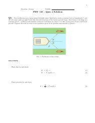
54 CHAPTER 2. FIELDS WITH SPINwhich commutates to all other γ-matrices,{γ 5 , γ µ } = 0.From this new matrix γ 5 , one can define the projective operators, P ± ,that project out states in the four-solutions ψ in our previous Dirac-Paulirepresentation and also in the Weyl representation,γ i =( 0 σi−σ i 0), γ 0 =( 0 II 0), γ 5 =( −I 00 IIt is easier to see the projection in the Weyl (or chirality representation),where the projector operator just flips the spinor in the appropriate direction.For example, for the free-particle solution of the previous exercise,putting it back in 2.1.3, we can eliminate the exponential dependence andwork only with the spinor part on χ s and φ r . We can then see explicitly theaction of the projector operator:P − = 1 ( ) ( ) ( )1 0 χ2 (1 − γ s χs5)ψ =0 0 φ r = → Left − handed.0P + = 1 ( ) ( ) ( )0 0 χ2 (1 + γ s 05)ψ =0 1 φ r =φ r → Right − handed.For the sake of completeness in analyzing the parity in the Dirac equation,the parity operator for the Dirac equation is given by γ 0 ,(i̸∂ − m)ψ(x 0 , x) = 0,γ µ† = γ 0 γ µ γ 0 → γ µ (i̸∂ P − m)γ 0 ψ(x 0 , x) = 0,where we use the notation ̸A = γ µ A µ . Therefore, one has ψ P (−x, x 0 ) =γ 0 ψ(x, x 0 ).2.14 Propagators in The FieldScalar Field PropagatorThe scalar theory for the free field is given by the hamiltonian (density)).H = 1 2 Π2 + 1 2 (∇φ)2 + 1 2 m2 φ 2 , (2.14.1)and the respectively lagrangian (density),L = − 1 2 (∂µ φ) 2 − 1 2 m2 φ. (2.14.2)

2.14. PROPAGATORS IN THE FIELD 55The Feynman propagator is then∫∆(x − y) =d 4 k(2π) 4e ik(x−y)k 2 + m 2 − iɛ . (2.14.3)This propagator is the Green’s function for the Klein-Gordon equation,i.e. a solution of this equation (taking ɛ → 0),(−∂ 2 x + m 2 )∆(x − y) = δ 4 (x − y). (2.14.4)However we can evaluate ∆(x − y) explicitly by taking the k 0 integralin 2.14.3, which is a contour integral in the complex k 0 plane, where the 4-vector inner product is k(x − y) = k 0 (x 0 − y 0 ) − ⃗ k(⃗x − ⃗y) (in the Minkowskispacetime, this expression is not uniquely defined because of the poles, k 0 =± √ ⃗p 2 + m 2 ).In resume, the different choices of how to deform the integration contourlead to different sign for the propagator. Let us them calculate it explicitlyby the residue theorem. We choose the causal (retarded) propagator, as inthe contour in figure 2.14. The integral is zero if x or y are spacelike (ifx 0 > y 0 , i.e. x 0 is future of y 0 ). The integral is thenI = lim ɛ→0∫ ∞−∞∫= iθ(t − t ′ )d 3 ∫k ∞(2π) 3dk 02πe ik(x−y)−∞ − ⃗ k 2 − m 2 − (k 0 + iɛ) ,∫2dk 3 e ik(x−y) + iθ(t − t ′ ) d 3 ke −ik(x−y) .Using the formalism of functional integrals (writing the path integral), wecan evaluate the ground-state expectation value of the time-ordered productof our scalar fields in terms of this propagator,〈0|T φ(x 1 )φ(x 2 )|0〉 = −i∆(x 2 − x 1 ). (2.14.5)A little comment for future discussions in the Feynman diagrams is thatthe result in 2.14.5 is generalized for many fields by the Wick’s Theorem,〈0|T φ(x 1 )...φ(x 2n )|0〉 = −i n ∑ pairs∆(x i1 − x i2 )...∆(x i2n−1 − x i2n ). (2.14.6)Now that we understand the propagator for the scalar field, we cancompute it for the Dirac field.

56 CHAPTER 2. FIELDS WITH SPINFree Fermion PropagatorWe are going to consider the free Dirac field,ψ(x) = ∑ ∫ [d 3 p b s (p)u s (p)e ipx + d † s(p)v s e −ipx] , (2.14.7)s=1,2¯ψ(y) = ∑s=1,2∫d 3 p ′[ b s ′(p ′ )ū s ′(p ′ )e ip′y + d † s ′ (p ′ )v s ′e −ip′ y ] , (2.14.8)where we sum on the spin polarization. The annihilation operators are givenbyand the anticommutation relations areb s (p)|0〉 = d s (p)|0〉 = 0, (2.14.9){b s (p), b † s ′ (p ′ )} = (2π) 3 δ 2 (p − p ′ )2ωδ ss ′, (2.14.10){d s (p), d † s ′ (p ′ )} = (2π) 3 δ 2 (p − p ′ )2ωδ ss ′, (2.14.11)with zero to all other combinations.Now we want to compute the Feynman propagatorS(x − y) αβ = θ(x 0 − y 0 )〈0|{ψ α (x) ¯ψ β (y)|0〉, (2.14.12)= i〈0|T ψ α (x) ¯ψ β (y)|0〉, (2.14.13)where θ(t) is the step function and T is the time-ordered product,T ψ α (x) ¯ψ β (y) = θ(x 0 − y 0 )ψ α (x) ¯ψ β (y) − θ(y 0 − x 0 ) ¯ψ β (y)ψ α (x).(2.14.14)The minus sign in the last result comes from the anticommutation propriety,{ψ α (x), ¯ψ β (y)} = 0 when x 0 ≠ y 0 , and we will discuss the causalityin the end. To derive the propagator and show that it obeys causality, letus now insert 2.14.8 into 2.14.14,〈0|ψ α (x) ¯ψ β (y)|0〉 = ∑ ∫d 3 pd 3 p ′ e ipx−ip′y u s (p) α ū s ′(p ′ ) β 〈0|b s (p)b † s(p ′ )|0〉,′s,s ′= ∑ s,s ′ ∫= ∑ s,s ′ ∫d 3 pd 3 p ′ e ipx−ip′y u s (p) α ū s ′(p ′ )(2π) 3 δ 3 (p − p ′ )2ωδ ss ′d 3 pe ip(x−y) u s (p) α ū s ′(p ′ ) β .

2.14. PROPAGATORS IN THE FIELD 57Using the result of the sum of all spin polarizations,∑u s (p)ū s (p) = −̸p + m, (2.14.15)we finally have∫〈0|ψ α (x) ¯ψ β (y)|0〉 =In the same fashion,〈0|ψ α (x) ¯ψ β (y)|0〉 = ∑ s,s ′ ∫s∑v s (p)¯v s (p) = −̸p − m, (2.14.16)s= ∑ s,s ′ ∫= ∑ s,s ′ ∫=∫d 3 pe ip(x−y) (−̸p + m) αβ .d 3 pd 3 p ′ e −ipx+ip′y v s (p) α¯v s ′(p ′ ) β 〈0|d s (p)d † s ′ (p ′ )|0〉,d 3 pd 3 p ′ e −ipx+ip′y v s (p) α¯v s ′(p ′ )(2π) 3 δ 3 (p − p ′ )2ωδ ss ′,d 3 pe −ip(x−y) v s (p) α¯v s ′(p ′ ) β ,d 3 pe −ip(x−y) (−̸p − m) αβ .These two results can be combined in the time-ordered product, and weget∫〈0|T ψ α (x) ¯ψ d 4 pβ (y)|0〉 = −i(−̸p + m) (2π) 4 ei(p(x−y) αβp 2 + m 2 − iɛ = iS(x − y) αβ,recovering the Feynman propagator.Dirac operator(−i̸∂ + m)S(x − y) = δ 4 (x − y).This is of course the inverse of theAgain, let us consider the vacuum expectation value of a time-orderedproduct of more than two fields. We must have an equal number of ψ and¯ψ to get a nonzero result. Concerning the statistics, there is an extra minussign if the ordering of the fields in their pairs is odd permutation of theoriginal ordering. For instance,〈0|T ψ α (x) ¯ψ β (y)ψ γ (z) ¯ψ δ (w)|0〉 = −i 2[ S(x − y) αβ S(z − w) γδ−S(x − w) αδ S(z − y) γβ],

58 CHAPTER 2. FIELDS WITH SPINLet us analyze these results. We recognize the right side integral of ourderivations to be the commutator of two scalar fields ∆ KG (x − y), hence theanticommutator of the Dirac theory isi∆ αβ (x − y) = (−i̸∂ + m)i∆ KG (x − y),and it will vanishes since ∆ KG (x − y) vanishes at spacelike separations,concluding that Dirac theory is causal.From reference [PS1995], we see that if we had quantized the Dirac theorywith commutators instead of anticommutators, we would have a violationof causality, with the exponentials of 2.14.8 summing up instead of having aminus sign and we would have a decaying at equal time and long distances( ˜∆ → emx , mx → ∞). In another words, if the theory were to be quantizedx 2with commutators, the field operators would not commute at equal time atdistances shorter than the Compton wavelength, violating the causality.We had just obtained the Spin-Statistic Theorem, , which states thatfields with half-integer (integer) spin must be quantized as fermions (bosons),making use of anticommutators (commutators). If the theory is quantizedwith the wrong spin-statistic connection, it either becomes non-local (nocausality) or it has no ground state (spectrum with negative norm).

Chapter 3Non-Abelian Field TheoriesLet us generalize the concept of local phase invariance to the Lagrangiandensities with N identical spinor fields that posse global symmetry U(N),ψ ′ i(x) = U ij ψ j (x).If U → U(x), the Dirac Lagrangian is no longer invariant. For N = 1,it is possible to recover the QED case, (2.8.4), however,, for N > 1, thechanges on the Lagrangian are only canceled if one introduces nonabeliangauge fields, also known as Yang-Mills fields, (A µ ) ij .Starting with Lagrangians with global spin U(N) = U(1) × SU(N), onehas a set of N Dirac fields ψ i , with mass m ψ and N scalars fields φ i withmass m φ . The gauge fields are N × N matrices,(A µ ) ij =∑(T a ) ij A µ a(x) ¯ψ, (3.0.1)N 2 −1a=1where T a are the generators of SU(N) in the N × N (fundamental) representation.For this expression to be consistent, A µ should be an elementof the Lie algebra, where the number of gauge fields is the dimension of thegroup. The normalization is chosen to betr (T a T b ) = 1 2 δ ab.The covariant derivative is(D µ [A]) ij = δ ij ∂ µ + ig(A µ ) ij , (3.0.2)D = (̸∂ + iɛ̸A). (3.0.3)59

60 CHAPTER 3. NON-ABELIAN FIELD THEORIESThe field strength (also a matrix) isF µν = δ µ A ν − ∂ ν A µ + ig[A µ , A ν ],=N∑2 −1The Yang-Mills Lagrangian isaF µν,a T a .L Y M = ¯ψ i {[iD µ (A)] ij γ µ − mδ ij }ψ j , (3.0.4)where the covariant derivative was defined in (3.0.3). One can make globalinvariance (phase U(1) and global SU(N)) by local combining it to thevector fields gauge theories. A resume of the simplest Yang-Mill’s theoryfactors can be seen in the table 3.1.COMPONENTYANG-MILLSFieldsDirac ψ i , Scalar φ iGenerators T a , a = 1, ..., n 2 − 1Commutator[T a , T b ] = if abc T cMatrix to the Fields A µ (x) ij = ∑ n 2 −1a=1 Aaµ a(x)(Ta R ) ijCovariant Derivative D µ [A] ij = δ ij ∂ µ + igA µ (x) ijField Strength F µν = ∂ µ A ν − ∂ ν A µ + ig[A µ , A ν ]Fields in components F µν = ∑ n 2 −1a=1 F µν,aTaRTable 3.1: The Yang-Mills theory.3.1 Gauge TransformationsThe infinitesimal gauge transformations of the vectors A µ are given byU R (x) = e ig ∑ N 2 −1a−1 Λ a(x)T R a,N∑2 −1= 1 + ig δΛ a (x)T a ,a=1= [1 + igδΛ(x)] ij .

3.2. LIE ALGEBRAS 61The A µ transformations are constructed in a way to give the form invariantLagrangian,Finite → A ′µ = UA µ U −1 + i g (∂µ U)U −1Infinitesimal → A ′µ = A µ − ∂ µ δΛ(x) + ig[δλ(x), A µ (x)],where the first two terms are the same as in any theory with U(1) gaugeinvariance and the last term is new for non-abelian theories. To complete theLagrangian (3.0.4), we need to supply a new term which is a generalizationof the Maxwell field density, this field strength transforms covariantly asF ′ µν(x) = U(x)F µν U −1 ,with the following components, where the last term is Yang-Mills field,F µν = U(x)F µν,a t a ,F ′ µν,a = ∂ µ A µ,a − ∂ ν A µ,a − gC abc A µ,c A ν,c ,The gauge invariant Lagrangian is thenL Y M = − 1 4∑aF µν,a F µνa ,= 1 2 tr[F µνF µν ].Putting all this together, the Lagrangian invariance under SU(N) forthe spinor is and a scalar isL SU(N) = |D µ (A) ij φ k | 2 − m 2 φ |φ|2 + ¯ψ i (i̸D[A] ij − m φ δ ij )ψ j − 1 2 Tr [F µν, F µν ].3.2 Lie AlgebrasIn compact Lie Algebras, that are the interest here, the number of generatorsT a is finite. Any infinitesimal group elementg can be written asg(α) = 1 + iα a T a + O(α 2 ),

62 CHAPTER 3. NON-ABELIAN FIELD THEORIESwhere[T a , T b ] = if abc T c (3.2.1)are the non-abelian generators commutation relation. If one of the generatorscommutes with all of the others, it generates an independent continuousabelian group ψ → e iα ψ, called U(1). If the algebra contains such commutingelements, it is a semi-simple algebra. Finally, if the algebra cannot bedivided into two mutually commuting sets, it is simple. The condition thata Lie Algebra is compact and simple restricts it to four infinity families and5 exceptions.Unitary Transformations of N-dimensional vectors For η, ξ n-vectors,with linear transformations η a → U ab η b and ξ a → U ab ξ b , this subgrouppreserves the unitary of these transformations, i.e. it preserves η ∗ aξ a .The pure phase transformation ξ a e iα ξ a is removed to form SU(N),consisting of all N × N unitary transformations satisfying det(U) = 1.The N 2 − 1 generators of the group are the N × N matrices T a underthe condition tr[T a ] = 0.Orthogonal Transformations of N-dimensional vectors The subgroupof unitary N × N transformations that preserves the symmetric innerproduct: η a E ab ξ b with E ab = δ ab , which is the usual vector product,so this is the rotation group in N dimensions, SO(N), or the rotationgroup in 2n + 1 dimensions, SU(2n + 1). There is an independent rotationto each plane in N dimensions, thus the number of generatorsare N(N−1)2.Symplectic Transformations of N-dimensional vectors The subgroupof unitary N × N transformations. For N even, it preserves the antisymmetricinner product η a E ab ξ b ,E ab =( 0 1−1 0where the elements of the matrix are N 2 × N 2),blocks, Sl(N), withN(N+12.RepresentationsIf the Lie algebra is semi-simple, the matrices t a r are traceless and the traceof two generator matrices are positive definite given bytr [T a r , T b r ] = D ab .

3.2. LIE ALGEBRAS 63Choosing a basis for T a which has D ab ∝ I for one representation meansthat it will be true for all representations:tr [T a r , T b r ] = C(r)δab. (3.2.2)From the commutation relations, one can write the totally anti-symmetricstructure constant asf abc = −iC(r) tr [ta r, t b r]t c r. (3.2.3)For each irrep r of G, there will be a conjugate ¯r given byt a r = −(t a r) ∗ = −(t a r) T , (3.2.4)if ¯r ∼ r then t ā r = Ut a rU † and the representation is real. The two mostimportant irreducible representations are the fundamental and the adjoint,which dimensions are given by table 3.2.Fundamental In SU(N), the basic irrep is the N-dimensional complexvector, and for N > 2, this irrep is complex. In SO(N) it is real andin Sl(N) it is pseudo-real.Adjoint This is the representation of the generators, r = G, and therepresentation’s matrices are given by the structure constants (t b c) ab =if abc where ([t b G , tc a]) ae = if bcd (t d G ) ae. Since the structure constants arereal and anti-symmetric, this irrep is always real.FUNDAMENTAL ADJOINT EXAMPLESSU(N) N, complex N 2 − 1 N=4, 4 and 15N(N−1)SO(N) N, real2N=4, 4 and 6N(N+1)Sl(N) N, pseudo-real2N=4, 4 and 10Table 3.2: Dimensions of the most important irreps of the compact andsimple Lie algebras.A good way of seeing the direct application of this theory on fields is,for example, the covariant derivative acting on a field in the adjoint representation,(D µ φ) a = ∂ µ φ a − igA a µ(t b G) ac φ c ,= ∂ µ φ a + gf abc A b µφ c ,

64 CHAPTER 3. NON-ABELIAN FIELD THEORIESand the vector field transformationA a µ → A a µ + 1 g (D µα) a .Casimir OperatorFor any simple Lie algebra, the operator T 2 = T a T a commutes with allgroups of generators:[T b , T a T a ] = (if bac T a + T a (if bac T c ),= if bac {T c , T a },= 0.For the adjoint representation,f acd f bcd = C 2 (G)g ab ,d(r)C 2 (r) = d(G)C(r),where, for example, for SU(2), C(r) = 1 2. ForSU(N), one has the quadraticCasimir operator coefficient,C 2 (r) = 1 (N 2 − 1)2 N3.3 Spontaneous Symmetry BreakingSo far the locally invariant Lagrangian involved only massless vector matrices.The spontaneous symmetry breaking makes it possible to the Lagrangianto acquire at once both local gauge invariance and massive vectors. The systemchooses a ground state, with a definitive but arbitrary direction, anychoice breaks the symmetry. While the ground states breaks the symmetry,the Lagrangian remains gauge invariant.Example: The SU(2) × U(1) ModelIn the Higgs mechanism, we postulate a scalar field with a internal symmetryU(1) or great, coupled to a gauge field. We choose a doublet of complexscalar fields φ i , i = 1, 2 and write the Lagrangian asL U(1) = (iD µ (A)φ ∗ )(iD µ (A)φ) − V (|φ|) − 1 4 F 2 ,D µ = ∂ µ + igA µ ,F µν = ∂ µ A ν − ∂ ν A µ ,

3.3. SPONTANEOUS SYMMETRY BREAKING 65Next step is to write explicitly theV (|φ|) = −µ 2 |φ| 2 + λ(|φ| 2 ) 2 ,which has its minimum in |φ 0 | 2 = ν22 = µ22λ, as in figure (3.1) and (3.2).Figure 3.1: The Higgs Potential for a real field.Figure 3.2: The Higgs Potential for a Complex field, in this case the minimumis the circle on |φ 0 |.The vacuum expectation value, 〈0|φ|0〉, is now different of zero and it isnot unique. Reparameterizing the scalar field toφ(x) = e i ξ(x)2VV + η(x)√2, (3.3.1)where V = √ µ λ, one performs the following replacement of the real andimaginary parts of φ i : Reφ, Imφ → ξ(x), η(x) (phase and modulus). The

66 CHAPTER 3. NON-ABELIAN FIELD THEORIESpotential is then independent of ξ(x) and one has only to replace |φ| by(3.3.1) in V . The mass will be generated to η(x) while ξ(x) will be massless,being only a physical degree of freedom.V (|φ| 2 ) = −µ 2 (V + η(x)√2) 2+ λ(V + η(x)√2) 4,= − µ24λ + µ2 η 2 (x) + √ λµη 3 (x) + λ 4 η4 (x),where the first term is constant and the third is the interaction. The fieldsξ(x) parametrize the position of φ around the 3-dimensional minimum whileη(x) measures the distance from this minimum. The transference of thephase degree of freedom from φ to A µ makes it appears as a mass, as it canbe seen at table (3.3)Start with Degree of Freedom End Degree of Freedomφ 2 η(x) 1A µ m=0 1 A µ m≠03V (|φ|) Gauge Invariant V (η) Gauge InvariantTable 3.3: Degree of freedom for spontaneous symmetry breaking of fields.The Lagrangian now has a mass term for the field, which is Proca-typemass. Spontaneous symmetry breaking of any kind implies the existence ofa massless scalar, the Goldstone boson. The difference to the Higgs is thethis would be a boson absorbed as a gauge field, i.e. vector.The theory in terms of new fields is simplified by canceling the nonabelianphase by a SU(2) gauge transformation, which is the Standard Model ofelementary particles is the electroweak group representation, with the gaugebosons W − , W + , Z 0 . This group transformation takes place byφ ′ = Uφ,B ′ µ = UB µ U −1 + i g (∂U)U −1 ,U(x) = e −iξ(x) σ 2v .Now the Lagrangian is independent of the fields ξ and its scalar part isL Higgs = |iD(B, C) ij φ j | 2 − V (|φ| 2 , (3.3.2)where |φ| 2 = |φ † | 2 + |φ 0 | 2 , (3.3.3)

3.3. SPONTANEOUS SYMMETRY BREAKING 67The potential and its extremal isV (|φ|) = −µ 2 |φ| 2 + λ|φ| 4 ,dV= −2µ 2 V + 4λV 3 = 0,d|φ| ∣φ=0V min = µ22λ .We write the four degree of freedom of φ as( )φ(x) = e −ξ(x) 0σ2 V +η(x) ,√2where the three ξ are three massive vectors and one η fields remains distancesfrom V min . The Lagrangian, ((3.3.3), is thenL Higgs = 1 2 [(∂ µη) 2 −2µ 2 η 2 ]−V λη 3 + λ 4 η4 + V 28. The phys-where the V 2 terms give the Proca mass: V 2 g 2 B1,22ical particles are then represented byW ± = 1 √2(B 1 ± iB 2 ),Z = −( sin θ W + B 3 cos θ W ),γ = ( cos θ W + B 3 sin θ W ),g ′where sin θ W = √g 2 + g . ′8 [g2 (B 2 1+B 2 2)+(g ′ C−gB 3 ) 2 ](V +η) 2 ,8, V 2 (g ′ C−gB 3 ) 2M Wcosθ w.The masses of the electroweak gauge bosons are then M W = V g2 , M z =

68 CHAPTER 3. NON-ABELIAN FIELD THEORIES

Chapter 4Quantum ElectrodynamicsIn this section we are going to understand and to derive the Lagrangianfor the theory of interaction of photons and matter the quantum electrodynamic,represented by (2.8.4). This theory is given by a vector fieldA µ (x) = C µ cos θ w + B µ 3 sin θ w.After the spontaneous symmetry breaking, the photon Lagrangian isMaxwell-form,This couples to fermions asL A = − 1 4 F 2 µν(A) − λ 2 (∂A)2 .L ferm (ψ F , A) = ∑ ¯ψF (i(̸∂ − ieQ F ̸A) − m F )ψ F ,where Q F is the charge of the fermion in units of positron charge (Q F =1, 2 3 , − 1 3 , 0). The L QED is then L A + L ferm .Because the minimum coupling, the term ¯ψAψ is not free. As a scalartheory, it makes it necessary to find the Green’s function 〈0|T (ψ(x), ψ(y)A µ (z), ...)|0〉to derive the S-matrix,L QED → Z[J µ (x), k α (y), ¯k β (z)] → S-matrix.By analogy to the scalars fields, one can write the generating functionalfor the Green’s functions,Z QED [J µ , k α , ¯k β ] =69W [J, k, ¯k]W [0, 0, 0] , (4.0.1)

70 CHAPTER 4. QUANTUM ELECTRODYNAMICSwhere W are the path integrals and J is the source. The path integral shouldbe over classical c-numbers for fields.∫W QED [A, k, ¯k] = [dA µ ][dψ α ][d ¯ψ β ]e i ∫ d 4 xL QED −i(J,A)−i(k,A)−i( ¯ψ,k) ,∫= [dA µ ]W [A, k, ¯k]e i ∫ d 4 x[L(A)− λ 2 (∂A)2] ,∫= [dψ][dψ]e i ∫ d 4 x ¯ψ[i̸D(A)−m]ψ e −i(ψ,k)−i(k,ψ) ,where the last two exponentials are the fermion Gaussian integral. We recallthe Gaussian scalar form,∫ ∞ n∏ω(j i ) = dx i e − 1 2 x iM ij x J −J k x k,=−∞i−1∏ n/2√det Me − 1 2 J k(M −1 ) kl J l.The Green’s function is thenn∏G(y i , x i ) = 〈0|T [ ψ ai (y i ) ¯ψ bi (x i )]|0〉,=i=1n∏ δ{[iδ(¯k ai , y i ) ][−ik bi(x i )]}Z[k, ¯k, A]| k=¯k=0 ,i=1which gives propagator for fermions∫1S F (z) =(2π) 4 d 4 ke −ikz 1̸k − m + iɛ ,∫1=(2π) 4 d 4 ke −ikz ̸k − mk 2 − m 2 + iɛ ,with ̸k̸k = k 2 . The charged scalar is∫W ψ [L, ¯L] = [dφ][dφ ∗ ]e −iS kg−i( ¯L,φ)−i(φ ∗ ,L) ,= W [0, 0]e −i ∫ W Z L∗ (ω)∆(ω−z)L(z) ,giving, finally, the generating functional for fermions∫W φ [A, k, ¯k] = DψD ¯ψe i ∫ d 4 y ¯ψ(i̸D(A)−m)ψ−i¯kψ−i ¯ψk ,∫1Z =DψDW [0, 0, 0]¯ψDAe i ∫ d 4 yψ(i̸D−m)ψ−¯kψ− ¯ψk−yA .

4.1. FUNCTIONAL QUANTIZATION OF SPINORS FIELDS 714.1 Functional Quantization of Spinors FieldsThe Grassmann variables defined at section (2.10) are now used in the fieldsψ, defined as a function of spacetime whose values are anticommuting number.We define this field in terms of orthonormal basis functions,ψ(x) = ∑ iψ i φ i (x),where ψ is the Grassmannian variable and φ is the four-component spinor.The Dirac two point correlation function is∫〈|T ψ(x i ) ¯ψ(x DψD ¯ψei ∫ d 4 x ¯ψ(iγ µ −m)ψ] ψ(x 1 )2 )|0〉 =¯ψ(x 2 )∫D ¯ψDψei ∫ d 4 x ¯ψ(iγ (4.1.1)µ −m)ψUsing the Gaussian integrals( ∏ ∫dθi ∗ dθ i )e −θ∗ i B ijθ j= ∏iib i= det B,if θ were an ordinary number, one would have (qπ)ndetB . Also( ∏ ∫dθi ∗ dθ i )θ k θl 4 e−θ∗ i B ijθ j= det B(B −1 ) kl .iOne can then calculate (4.1.1), where the denominator is det(iγ µ ∂ − m)and numerator is det(iγ µ −1∂ − m)iγ µ ∂−m. From this is possible to recover thepropagator for fermions,∫〈0|T ψ(x 1 ) ¯ψ(x d 4 k ie −ik(x i−x 2 )2 )|0〉 = S F (x 1 − x 2 ) =(2π) 4 ̸k − m + iɛ4.2 Path Integral for QEDThe QED Lagrangian with sources isL QED =∑ ¯ψ(i̸D[A] − m)ψ − 1 4 F 2 (A) − λ 2 (∂A)2 .flavorsWriting it considering only connected diagrams, i.e all lines connectedto some external point in the Green’s function, we getZ free [J µ , k α , ¯k α ] =W [J, k, ¯k]W [0, 0, 0] ,= e − ∫ w,z [ 1 2 J µ (w)G µν(w−z)J ν (z)+¯k α(w)S αβ (w−z)k β (z)] ,

72 CHAPTER 4. QUANTUM ELECTRODYNAMICSwhereW [J, k, ¯k] = W free e − ∫ d 4 y[−δ k (y)] α(γ µ ) αβ [iδJ µ(y)][iδ k (y)] .The greens functions are the variations of J, k, ¯k, and one sets all themequal to zero.4.3 Feynman Rules for QEDIn the same fashion as section 1.10, we can summarize the last results inrules for fermions in an external gauge field. As for charged scalar fields,fermions lines carries arrows, pointing from ¯ψ to ψ. The Feynman rules forQED are:• Distinguishable diagrams with continuous fermions lines.• For every fermion line, starting at z pointing to w, one adds i(S F (w −z)) αβ , which is i(2π) −4 ∫ d 4 k[(k − m) −1 ] ba .• For every vector lines, iG µνF(w − z).• For every vertex −ie(γ µ ) λσ , as a result of −ieQ f δ ff ′γ µ dc (2π)4 δ 4 ( ∑ i p i),where p i labels the momenta of lines flowing.• For each internal photon line, one adds the factor 1 ∫2π d 4 k 1k 2 −iɛ [−gµν +(1 − 1 λ ) kµ k νki 2ɛ ].• Sign rule: (-1) for every fermion loop and (-1) when exchanging pairingof external ψ, ¯ψ.In the momentum space, the rules are the similar with a few exceptions,• For every fermion line, starting at z pointing to w, one adds ∫• For every vector lines, ∫(d 4 k i(2π) 4 k+iɛ• For every vertex −ie(2π) 4 δ 4 ( ∑ i k i)(γ µ ) βα .k µ k ν− g µν + (1 − 1 λ).k 2 +iɛ )d 4 k i(̸k + m)(2π) 4 k 2 −m 2 −iɛ .

4.4. REDUCTION 734.4 ReductionThe use the results of the Green’s functions to to find the S-matrix, we needthe residues of single-particle pole defined by∫d 4 xe ipx 〈0|T (ψ(x) ¯ψ(0))|0〉.The reduction for e + e − → e + e − in terms of the T-matrix is given byS = 1 + iT , where() (iT (p ′ , λ ′ ) − , (q ′ , σ ′ ) + out ; (p, λ), (q, γ) ūα (p ′ , λ ′ ))( −¯vβ (q, σ))in =(R ψ (2π) 3 ) 1 2 (R ψ (2π) 3 ) 1 2(×G α ′ β ′ ,αβ(p ′ , q ′ uα (p, λ))( −vβ (q ′ , σ ′ )) ∣ ∣∣∣p, p, q) trun ×(R ψ (2π) 3 ) 1 2 (R ψ (2π) 3 ) 1 2 2 =p ′2 =q 2 =q ′ 2=m 2The two first parenthesis are the outgoing and incoming fermions andthe two last the incoming and outgoing fermions, respectively.For vectors, the rules are the same, to get the S-matrix: we go to theɛmomentum space, truncate it and multiply it by,µ (k), the incomingvector,ɛ µ (k ′ ) ∗(R A (2π) 3 ) 1 2, the outgoing vector.4.5 Compton Scatteringγe − → γe − .The S-matrix for the Compton Scattering is(R A (2π) 3 ) 1 2ɛ ′ν (l ′ ) ∗ ū β (p ′ , σ ′ )G trun ɛ µ (l) · u α (p ′ 1, σ).R A R ψ (2π) 6 .4.6 The Bhabha ScatteringThe Bhabha scattering is an example of tree level gauge theory cross section.e + e − → e + e − .The S-matrix level is gauge invariant (independent of gauge theory fixing),iM(p 4 , σ 4 , p 3 , σ 3 , p 2 , σ 2 , p 1 , σ 1 ) =

74 CHAPTER 4. QUANTUM ELECTRODYNAMICSFigure 4.1: The two tree Feynman diagrams of the Bhabha Scattering. Inthe internal line, µ and ν couple together by the propagator of the photon.The first diagram is the scattering exchange and the second the annihilationfollowed by a pair creation, All momentum are on-shell.There are two diagrams (figure 4.1),iM = (2π) 4 δ 4( 4∑ ) [(k µ ii)i×−ki=12 − m [−ieγµ ]k 4 − m−bd()i−|k 2 + k 4 | 2 − g µν + (1 − 1 λ ) 1|k 2 + k 4 | 2 ×(ii)−k 3 − m [−ieγµ ]k 1 − m ca− other diagrams where k 2 ↔ k 3 , b ↔ c.The Green’s function is always pure imaginary for tree diagrams and Tand M are always real. From the result of the reduction,T = σ 4( ∑ki) 1(2π) 6 M,

4.6. THE BHABHA SCATTERING 75where we only need to find M. From the diagrams,iM({p i , σ i }) = ¯v(p 2 , σ 2 )(−ieγ) µ v(p 4 , σ 4 ) ×1((p 2 − p 4 ) 2 − g µν + (1 − 1 λ )(p 2 − p 4 ) µ (p 2 − p 4 )) ν(p 2 − p 4 ) 2 ×ū(p 2 , σ 2 )(−ieγ) µ )u(p 1 , σ 1 ) −−¯v(p 2 , σ 2 )(−ieγ) µ )v(p 1 , σ 1 ) ×1((p 2 − p 1 ) 2 − g µν + (1 − 1 λ )(p 2 − p 1 ) µ (p 2 − p 1 )) ν(p 2 − p 1 ) 2 ×]ū(p 3 , σ 3 )(−ieγ µ )u(p 4 , σ 4 ) ,which still depends on the gauge fixing parameter λ. The Green’s functionalso depend on the gauge while the physical amplitudes does not. Theterms multiplied by λ are dropped and one needs to keep − gµνfor photonk 2propagation. Simplifying (4.1), the first diagram is( )= ¯v 2 (−eγ µ −ig µν)u 1(p 1 + p 2 ) 2 ū 3 (−eγ µ )v 4 .The second is( )= −¯v 2 (−eγ µ −ig µν)v 4(p 1 + p 4 ) 2 ū 3 (−eγ µ )u 1 .Hence, one has(M = ¯v 2 (−ieγ) µ 1)v 4(p 2 − p 4 ) 2 ū 3 (−ieγ) µ u 1 −(¯v 2 (−ieγ) µ 1)u 1(p 1 − p 3 ) 2 ū 3 (−ieγ) µ v 4 .The gauge invariance of the general result for the S-matrix is common toall orders in QED and the other gauges theories. In general, M can dependson all invariants p i p j , p i σ j , σ j σ k , they are all Lorentz invariant number. However,certain dependences are not allowed by parity of QED. For example,let us suppose we haveM ∝ A({p 1 , p 2 }) + σ i p j B({p i , p j }).In the frame σ 0 = 0 this changes the spin under xp − x. In transformedfields where x = −x, M = A − σ i p j B, not allowed in QED, however allowedin the weak interactions.The Feynman identity (a generalization of the Ward identity) isū(p 2 )(̸p 2 − p 1 )u(p 1 ) = 0.

76 CHAPTER 4. QUANTUM ELECTRODYNAMICS4.7 Cross SectionFor a fixed spin, the relations for M are the same as for scalars. We cannow compute the cross section for fermion+antifermion scattering,dσdt = 116πs(s − 4m 2 ) |M({p i, σ i })| 2 ,where t = (p 3 − p 1 ) 2 = (p 4 − p 2 ) 2 , s = (p 1 + p 2 ) 2 , u = (p 4 − p 1 ) 2 .4.8 Dependence on the SpinMost experiment involves non-polarized beams at the target, i.e. incoherentcombination of spins. For unpolarized σ’s, we average over initial state spinand then sum over the final state,• First we look to the general initial state: |A in 〉 = ∑ Ni=1 CA i |{σ i}〉,where N is the number of different spin states, for example, for twoparticles with spin-half, N = 4.• If we have a unpolarized beam for a particle process A → B, then|M A→B | 2 ∝ |〈B out |A in 〉| 2 ,N∑= Cj ∗ C i 〈σ j |B out 〉〈B out |σ i 〉.u,j=1• If there is no polarization, we average the C’s: 〈C i |Cj ∗〉 = 1 N δ ij, andone has 〈|M A→B | 2 〉 = 1 ∑N i |〈B out|σ i 〉| 2 , which is the average over theinitial states.• For the final states, just sum over B’s definitive spin. Applying toBhabha scattering, we then see the simplification in the unpolarizedcase (it is not necessary to compute M for the fixed spin).• Rather than calculate ¯v 2 γ ∗ v 1 , etc, we use the complex conjugate of theidentity γ 0 γ µ γ = (γ µ ) † . Hence, any factor (ū i , γ α1 , γ α2 , ...¯γ αn , u j ) ∗ =ū j γ 2n γ 2n−1 ...γ 1 u i . This will generate four therms in the Bhabha scattering,which are the four cut diagrams, related to the optical theorem.

4.8. DEPENDENCE ON THE SPIN 77Calculating for the first cut diagram, we havee 4 ∑s 2 {(¯v 2 γ µ u 1 )(ū 1 γ ν v 2 )(ū 3 γ 5 v 4 )(¯v 4 γ µ u 3 )}.sUsing the projection relations,∑(u i ) β (ū i ) α = ∑ ū β (p i λ)u α (p i λ) = (̸p 1 + m) αβ ,sλ∑(v i ) β (¯v i ) α = ∑ ¯v β (p k , λ)v λ (p j , λ) = (̸p 2 + m) αβ ,sλfinally givinge 4 ∑ {s 2s}Tr dirac [(̸p 1 + m)γ ν (̸p 2 + m)γ a ]. Tr dirac [(̸p 3 + m)γ µ (̸p 4 + m)γ nu ] .The following other three diagrams have: (b)-2 traces and (c), (d)-onetrace. For the second of the cut diagrams, we havee 4 ∑s 2 {ū β (p 3 , λ 3 )(γ µ ) βγ u γ (p 1 , λ)ū λ (p 1 , λ 1 )(λ τ ) γτ u τ (p 3 , λ 3 )},sand the only trace is given by the piece in the middle,u λ (p 1 , λ)ū λ (p 1 , λ 1 ) = (̸p 1 + m) λσ .It is straightforward to find the other two cut diagrams.

78 CHAPTER 4. QUANTUM ELECTRODYNAMICS4.9 Diracology and Evaluation of the TraceTo calculate the traces of the diagrams in the Feynman, we define usefulproprieties of the Dirac matrices,tr {̸a̸b} = 2ab,tr γ µ = 0,tr (odd numbers of γ) = 0,tr [γ 5̸a̸b̸c̸d] = 4iɛ µνλν a µ b ν c λ d σ ,tr [̸a̸b̸c̸d] = 4(abcd + adbc − acbd),tr [ ∑ n−1∑̸a i ] = a n a ( i − 1)i−1 Trii=1γ 5 = iγ 0 γ 1 γ 2 γ 3 ,(γ 5 ) 2 = 1,(γ 0 ) † = γ 0 ,(γ µ ) † = γ 0 γ µ γ 0 ,{γ 5 , γ µ } = 0,̸a̸b = ab − 2ia µ S µν b ν ,S µν = i 4 [γµ , γ ν ],γ µ̸aγ µ = −2̸a,γ µ̸a̸bγ µ = 4ab,γ µ̸a̸b̸cγ µ = −γ µ̸a̸bγ µ̸c + 2̸c̸a̸b,= −s̸c{̸a, ̸b} + 2̸c̸a̸b,= −2̸a̸b̸c,{̸a, ̸b} = 2ab.

4.9. DIRACOLOGY AND EVALUATION OF THE TRACE 79andNow, we estabilish the follow relations,tr M ab = M a a ,tr γ µ = 0,tr γ 5 = 0,tr γ µ γ ν γ λ = 4g µν ,tr γ µ γ ν = 0,tr ̸a̸b = 4g µν ,tr γ 5 γ µ γ ν γ λ γ σ = 4iɛ µνλσ ,tr γ µ γ ν γ λ γ σ = 4(η µν η ρσ η ρσ − η µρ η νγ + η µσ η νρ ),tr (̸a 1̸a 2̸a 3̸a 4 ) = 4[(a 1 a 2 )(a 3 a 4 ) − (a 1 a 3 )(a 2 a 4 ) + (a 1 a 4 )(a 2 a 3 )],n−1∑tr (̸a 1̸a 2 ...̸a n ) = (a n .a i )(−1) i−1 tr (̸a 1̸a 2 ...̸a n−1 ).i=1Finally, we evaluate the traces,t b 1 µν = Tr [γ ν (̸p 1 + m)γ µ (̸p 3 + m)],= Tr [γ ν̸p 1 γ µ̸p 3 ] + m 2 Tr [γ ν γ µ ],= 4(p ν 1p µ 3 + pν 3p µ 1 − gνµ p 1 p 3 ) + 4m 2 p 1 p 3 .t b 2 µν = Tr [γ ν (̸p 2 + m)γ µ (̸p 4 + m)],= Tr [γ ν̸p 2 γ µ̸p 4 ] + m 2 Tr [γ ν γ µ ],= 4(p ν 2p µ 4 + pν 4p µ 2 − gνµ p 2 p 4 ) + 4m 2 p 2 p 4 .The full trace results to be a Lorentz invariant,T b = t b 1 µν (t b 2) µν= 16(p ν 1p µ 3 + pν 3p µ 1 − gµν p 1 p 3 )(p 2ν p 4µ + p 4ν p 2µ − g µν p 2 p 4 ) − 2m 2 (p 1 p 3 + p 1 p 3 ).Finally, we are in the very moment we can calculate the cross section,σdt = 2πα 2s(s 2 − 4m) { 1s2[(u − 2m 2 ) 2 + (t − 2m 2 ) 2 + 4m 2 s]+ 1 t 2 [(u − 2m 2 ) 2 + (s − 2m 2 ) 2 + 4m 2 s]+ 1 st[(u − 2m 2 ) 2 + 4m 2 (u − 2m 2 )] },

80 CHAPTER 4. QUANTUM ELECTRODYNAMICSwhere α = e24πand the Mandelstam variables ares = (p 2 + p 2 ) 2 ,t = (p 1 − p 3 ) 2 = (p 2 − p 4 ) 2 ,u = (p 1 − p 4 ) 2 = (p 2 − p 3 ) 2 .The behavior of the cross section in terms of the center of mass scatteringangle is derived from (4.9.1) for the spin average case with equal massparticles. Let θ be the center of mass angle between p i and p 3 , we rewritethe Mandelstam variables ass = 4E 2 ,t = −4(E 2 − m 2 ) sin 2 θ 2 ,u = −4(E 2 − m 2 ) cos 2 θ 2 .The previous calculation is simplified when we take the limit m → 0,which is the same limit which E and themoment transfered go to zero (fora fixed m). There is no specified spin dependence but the answer dependson the spin of the field.

Chapter 5Electroweak TheoryThe electroweak theory is represented by the LagrangianL EW = − √ g ∑ [ū (1)1 ̸W + l (L)2i+ ¯l]i̸W − u (L)i−gcosθ Wcharged∑neutral[]ū (1)1 ̸Zu(L) (L)i+ ¯li̸Z(γ 5 + 4sin 2 θ W − 1) .It consists of two parts, a charged current and interactions, couplingcharged leptons to neutrinos (only left-handed), and a ]it neutral current,coupling Z boson to neutrinos or charged leptons (left-handed and righthanded).The relevant vertice areThe propagator is(i̸k − m)− ig2 √ 2 [γµ (1 − γ 5 )] βα ,−ig [γ µ (1 − γ 5 )] βα ,2cosθ W−ig [γ µ (γ 5 + (4sin 2 θ N − 1))] βα .4cosθ Wαβi(q 2 − M 25.1 The Standard Model− g µν + q µq νM 2 ).The Standard Model of Particles is represented by three gauge field theories,SU(3) × SU(2) × U(1). The group and fields couplings are described in thetable 5.1.81

82 CHAPTER 5. ELECTROWEAK THEORYSU(3) SU(2) U(1)G µ a, a = 1, ..., 8 B µ b,b = 1, 2, 3. CµG are gluons B is W ± and Z C is γg s g g ′Table 5.1: The Standard Model.For each Dirac and scalar field, one must still specify how they couple.U(1) Is related to the charge, generates the phase transformation on thehypercharge Y (e i Y 2 α(x) ). SU(2) is related to the electroweak interactions,giving by the Z, W ± bosons.The Lagrangian of the Standard Model isL SM = L vectors + L higgs + L quarks + L leptons ,L vectors = − 1 2 Tr SU(3)[F 2 µν(A)] − 1 2 Tr SU(2)[F 2 µν(B)] − 1 4 F 2 µν(C).where the two first terms are bosons and the two last fermions.The general form of the covariant derivative isD µ [A, B, C] = ∂ µ + ig s A µ,a T (R3 f )a + igB µ,b T (R2 e)b+ ig ′ Y 2 C µ.The Standard Model distinguishes left-handed and right-hand parts ofthe Dirac field, whereψ L = 1 2 (I ∓ γ 5)ψ.Singlets fields (under SU(3), SU(2), U(1)) have a missing term D α . Forexample, leptons are singlets under SU(3), and other cases can be seen inthe table 5.2.R (3)fR e(2) YqR k 3 1,1 4/3, -2/3qL k 3 2 (u and d) 1/3lR k 1 1,1 0,-2lL k 1 2 (ν e and e) -1φ 1 2 1Table 5.2: Summary of the representations of the Standard Model.

5.1. THE STANDARD MODEL 83Hypercharge ConstructionThe way we represent the hypercharge in the gauge group formalism is bywritingQ EM = Y 2 + ISU(2) L3 ,where I 3 is equal to 1/2 for U l , µ l and -1/2 for d l , l. The symmetry SU(2)does not allow a Dirac mass term: m ¯ψψ = m( ¯ψ L ψ R + ¯ψ R ψ L ), since ψ Land ψ R transforms differently. These fields gets mass by the same Higgsmechanism of vectors. The Higgs fields are represented asΦ =( φ † , I 3 = 1 2φ 0 , I 3 = − 1 2).

84 CHAPTER 5. ELECTROWEAK THEORY

Chapter 6Quantum Chromodynamics6.1 First Corrections given by QCDThe Lagrangian of QCD isL = ¯ψ i (iγ µ δ µ − m)ψ i − g( ¯ψ i γ µ T aijψ i )G a µ + 1 4 Ga µνG µνa . (6.1.1)In this section, we will calculate the first corrections due the strong force:the first-order radiation of gluons jets on the process e + e − → g¯qq, a QCD’sprocess 1 . This can be seen as an coupling terming of fermions to gluons atthe Lagrangian,g ¯ψ fi γ µ γ fi B µ , (6.1.2)with color indexes i = 1, 2, 3 and f the quark flavors. One can then calculatethe cross section for emission of one gluon. Writing the four-momentum ofthe equation as q µ = q 0 , ⃗q, and the momentum of quark, anti-quark andgluon as k µ i − (ω i, ⃗ k), i = 1,2 and 3, the ratio of the center-of-mass energyof the particle i to the maximum available energy is given byx i = 2k iqq 2= 2E i√ s, (6.1.3)where ∑ x i = 2. To write the differential cross section, equation 6.1.4, oneneeds to calculate the phase space and matrix |M| 2 . From 6.1.3 one cancalculate the range of integration, finding 0 ≤ x q , x 2 ≤ 1 − µ q .85

86 CHAPTER 6. QUANTUM CHROMODYNAMICSdσ n = 1 q 2 [1 4∑spins∫|M| 2 ][Π n ]. (6.1.4)Choosing the frame where ⃗q = 0, one has k 1 +k 2 +k 3 = 0, the three-bodyphase space is given by∫ ∫d 3 k 1 d 3 k 2Π 3 =(2π) 5 δ(q 0 − ω 1 − ω 2 − ω 3 ), (6.1.5)8ω 1 ω 2 ω∫31=32π 3 dω 1 dω 2 σ(q 0 − ω 1 − ω 2 − ω 3 ), (6.1.6)q 2 ∫=128π 3 dx 1 dx 2 . (6.1.7)Calculating explicitly the two Feynman diagrams with emission of onegluon, squaring M, finding the two traces, electron (pure QED) and quarks(some extra tricks, see [PS1995]), one has14∑spins|M| 2 = 1 e4( 4 g 2 Q 2 )Fq 4 Tr [̸pγ µ̸pγ α ] Tr [̸pΛ βµ̸pΛ αβ ], (6.1.8)= e4 g 2 Q 2 F4q 4 I µα G µα . (6.1.9)Gathering everything on 6.1.4, one has the differential cross section:dσ = e4 g 2 Q 2 F4q 4 1256π Iµα ∫= 2α2 α 2 s3Q 2 fq 2 ∫dx 1 dx 2 G µα , (6.1.10)8(x 2 1 + x2 2 )(1 − x 1 )(1 − x 2 ) dx 1dx 2 . (6.1.11)d 2 σdx 1 dx 2= 8σ2 σ 2 sQ 2 f3q 2 8(x 2 1 + x2 2 )(1 − x 1 )(1 − x 2 ) . (6.1.12)Integrating this on the range 0 ≤ x 1 , x 2 ≤ 1 gives an integral that diverges.One then sets the range of integrations are the infrared divergencesas µ → 0, and integrating with µ ≠ 0 one gets the infrared terms proportionalto ln( µ q), which are related to the infrared cut of QCD. These singularitiesare not physical but the breakdown of perturbation theory, meaningthat the mass of quarks and gluons are never on-shell, as was supposed

6.2. THE GROSS-NEVEU MODEL 87on these calculations (e.g. ω i cannot be of the same order of the hadronmasses).The 2-3 kinematics collapses to an effective 2-2 due to an emissionof soft gluon or to collinear splitting of a parton on two. There are then twopossible emissions, soft (when √ ω 3s→ 0) and collinear (when θ i3 , (1 − x i ) → 0from (1 − x i ) = x jω 3q(1 − cos θ j3 )).6.2 The Gross-Neveu ModelThe Gross-Neveu model is a quantum field theory model of massless Diracfermions with one spatial and one time dimension, with an attractive shortrangepotential, where fermion pairs composite condensates to break Z 2 -symmetry and acquire mass. It was introduced as a toy model for quantumchromodynamics.The Lagrangian of the model is given byL = ¯ψ i i̸∂ψ i + 1 2 g2 ( ¯ψ i ψ i ) 2 .This theory is invariant under ψ i → γ 5 ψ i and the chiral symmetry forbidsthe appearance of fermions mass.Proof. ¯ψi ψ i = ψ † i γ0 ψ i = ψ † (γ 5 γ 0 γ 5 )ψ i = −ψ † γ 0 ψ i = − ¯ψ i ψ i . Therefore wesee that ¯ψ i ψ i = const. Same proof can be made for ¯ψ i i̸∂ψ i . This is a Z 2symmetry.The theory is renormalizable in two dimensions.Proof. The mass dimension in a theory in D-dimensions is D−12. The spacetimevolume has dimension −D. The Lagrangian density has mass dimensionD. Therefore, for D = 2, we have D−12= 1 2(−ɛ). Since the four-fermionoperator has dimension=2, g is dimensionless and renormalizable.6.3 The Parton ModelThe intrinsic scheme of the elementary particles in nature is given by theircomposed quarks. We call parton all the quarks and gluons of inside aparticle. We represent the parton distribution in the vacuum sea byu s (x) = ū s (x) = d s (x) = ¯d s (x) = s s (x) = ¯s s (x) = s(x). (6.3.1)On another hand, we represent the valence quarks, such as in the proton,u(x) = u v (x) + u s (x), (6.3.2)d(x) = d v (x) + d s (x). (6.3.3)

88 CHAPTER 6. QUANTUM CHROMODYNAMICSSumming all the contribution of these partons, it is necessary to recovercharges, baryon number and strangeness,∫ 10∫ 10∫ 10[u(x) − ū(x)]dx = 2, (6.3.4)[udx) − ¯d(x)]dx = 1, (6.3.5)[s(x) − ¯s(x)]dx = 0. (6.3.6)The presence of gluons emissions is signaled by a quark jet and a gluonjet in the final state, either in the direction of the virtual photon (p T ≠ 0).Deep Inelastic ScatteringAt a very high resolution (when the transfered momentum q 2 is large), thenucleon can be resolved as a collection of almost non-interacting point-likeconstituents, the partons. When the resolution scale λ of the effective probeq is smaller than the typical size of the proton (∼ 1 fm), the internal structureof the proton is probed and we have the deep inelastic regime (DIS), 6.1-a.Defining Q 2 = −q 2 > 0 as the off-shell momentum of the exchanged photon,the resolution scale is λ = Q .Figure 6.1: a)DIS, b) Elastic scattering.The electron-quark scattering, e − (k)+q(p q ) → e − (k ′ )+q(p ′ q), is given bythe QED differential cross section (partonic massless limit (ŝ + ˆt + û = 0)),where the matrix element squared for the amplitudes are∑|M| 2 = 2e 2 qe 4 ŝ2 + û 2ˆt 2 .In terms of the Mandelstam variables, ŝ = (k + p q ) 2 , ˆt = (k − k ′ ) 2 , û =(p q − k ′ ) 2 . In the frame which the proton is moving very past, P ≫ M, we

6.3. THE PARTON MODEL 89can consider a simple model where the photon scatter a pointlike quark withɛ fraction of the momentum vector p = ξP . The deep inelastic kinematicsare ˆt = q 2 , û = ŝ(y − 1), ŝ = ξQ 2 /xy. The massless differential cross sectionis thendˆσdˆt = 1 ∑|M| 216πŝ 2 ,where, substituting the kinetic variables,dˆσdQ 2 = 2πα2 e 2 qQ 4 [1 + (1 − y) 2 ].The mass-shell constraint for the outgoing quark p ′2q = 0 suggest thatthe structure function probes the quark with ξ = x. With s the square ofthe the center-of mass energy of the electron-hadron, the invariant ŝ isŝ = (p + k) 2 ∼ 2p . k ∼ xs.Writing ∫ 10dxδ(x − ξ) = 1 we have the double cross section for the quarkscattering process,d 2ˆσdxdQ 2 = 4πα2Q 4 [1 + (1 − y)2 ] 1 2 e2 qδ(x − ξ).The event distribution is in the x − Q 2 plane. The parton distributionfunctions (PDFs) parametrizes the structure target as ’seen’ by the virtualphoton and which are not computable from first principles through perturbativecalculations.The Bjorken limit is definite as Q 2 , q → ∞, with x fixed. In this limit thestructure functions obey an approximate scaling law, i.e. they only dependon x, not in Q 2 , as we can see in figure 6.2. Bjorken scaling implies thatthe virtual photon scatters off pointlike constituents, since otherwise thestructure functions would depend on the ratio Q/Q 0 , some length scale.Dividing it by (1 + ( Q2xs )2 )/Q 4 , we remove the dependence of the QEDcross section and the result is independent of Q 2 . The result is that thestructure of the proton scales to an electromagnetic probe no matter howhard it is probed.We see an anti-screening effect where the coupling constant appearsstrong at small momenta, behaviors called asymptotic freedom and belongingto a non-abelian gauge theory. These are the only field theory withasymptotic freedom behavior with interacting vector bosons which couldbind the quarks. This gauge theory confirmed the Bjorken scaling, with theevolution of the coupling very slow, following a logarithmic distribution inmomentum. The scaling violations corresponds to a slow evolution of theparton distributions F i (x) over a logarithmic scale Q 2 .

90 CHAPTER 6. QUANTUM CHROMODYNAMICSFigure 6.2: Bjorken scaling on e − p DIS by the SLAC-MIT experiment, range1 GeV 2

6.3. THE PARTON MODEL 91Figure 6.4: The up PDF from valence and sea. The Q 2 dependence is largefor small x and small Q 2 .The Running CouplingIn the previous simple parton model, the structure functions scale in theasymptotic (Bjorken) limit Q 2 → ∞. In QCD, next to the leading order inα s , this scaling is broken by logarithms of Q 2 . A quark can emit a gluondkTand acquire large k T with probability proportional to α 2 s . The integralkT2extend up the kinetic limit kT 2 ∼ Q2 and gives contributions proportional toα s Q 2 , breaking the scaling.The screening behaviors on QED is giving by summing the higher ordercorrections in terms of the general form α n [log(Q 2 /Q 2 0 )]m and retaining onlythe leading logarithm terms (m = n). Therefore the vacuum polarizationaffects the coupling in QED asα(Q 2 ) =1 − α(Q2 0 )3πα(Q 2 0 )log(Q 2Q 0),the leading logarithm approximation.For QCD, since gluons also emit additional gluons and similar chargesattract themselves, the effect is anti-screening, the effective color chargedecreases as one probes the original quark. Therefore, this phenomena ofasymptotic freedom is given by the QCD running coupling,α s (Q 2 ) =α s (µ 2 )1 + αs(µ2 )12π(11N c − 2N f ) log(Q 2µ 2 )where N c is the number of color charges, N f the number of quarks flavorsand µ the renormalization scale. To make α s independent of the renormal-

92 CHAPTER 6. QUANTUM CHROMODYNAMICSization scheme, we introduce a scale Λ 2 QCD ,Λ 2 QCD = µ 2 e−12π(11Nc−2N f )αs(µ ) ,which experimentally is ∼ 200. In this QCD scale, the coupling constantcan be written asα s (Q 2 12π) =(11N c − 2N f )log(Q 2 /Λ 2 QCD ),where we see α s → 0 when Q 2 → ∞ and when Q 2 ≫ Λ 2 QCDinteractions.we have hardFigure 6.5: At Q 2 increases, it is possible to probe shorter distances. Atlarge Q 2 , the large x quarks are more likely to loose energy due to gluonradiation.Leading Log ApproximationCollinear photon emission in QED at high energies is already associatedwith mass singularities and it leads to an analog of parton distribution forelectron. Gribov and Lipatov showed that in a field theory with dimensionlesscoupling α, the DIS structure functions are represented as a sum ofRutherford cross sections og lepton scattering the point-like charges particle,weighted by a parton density F f i (x).Logarithmic deviations from the true scaling behavior had been predictedfor the PDFs, reveling the internal structure of PDFs which corrections aregiven by F f i (x, logQ2 ). Physically: DIS with a photon with Q 2 correspondto the scattering of that virtual photon on a quark of size 1/Q. From QCDbremsstrahlung, we havedω ∝ α 2 ∫ Q 2dk⊥2k⊥2 ,

6.4. THE DGLAP EVOLUTION EQUATIONS 93therefore the collinear photon emission cost a factor not of α but α log(s/m 2 ), and multiple collinear photons gives contributions of order (α log(s/m 2 )) m .therefore it makes the total probability of extra parton production large,since for α 2 ≪ 1, log Q 2 is high enough and ω ∝ α 2 log Q 2 ∼ 1. In QCD,the corresponding factor for collinear gluon emission is α s (Q 2 ) log Q2.µ 2In QED, when k 2 → 0, we can write the expansion for g µν in termsof massless polarization vector and when the singular term as the photonmomentum q goes on-shel is given by −igµν → +iq 2 q∑i 2 ɛµ T i ɛν T iin the calculus ofthe amplitudes, decoupling the photon/electron emission vertex. The finalcross section is giving by∫ 1σ(e − X → Y ) = dz α0 2π log s [ 1 + (1 − z)2 ]m 2 z× σ(γY → Y ),=∫ 10dz F γ (z) × σ(γX → Y ).Considering the limit of the divergence z = 0 = 1 − x, the soft partonemission or infrared divergent, we see it is balanced by negative contributionsfrom diagrams with soft virtual photons. Thus, to order α, the partondistribution of electrons has the formF γ = δ(1 − x) + α 2π log s ( 1 + x2)m 2 1 − x − Aδ(1 − x) , (6.3.7)where the first delta is the zeroth order of the expansion and A we willexplicitly calculate in the following sections.6.4 The DGLAP Evolution EquationsThe hadron evolve with energy Y = log(1/x), and for some values of (Q 2 , x),although the hadron is no longer perturbative, the evolution still is (exceptfor low Q 2 ). Therefore, we can construct evolution equations in this two thetwo variables of the phase space: log(1/x) and logQ 2 .In figure 6.6 we see that when Q 2 , Y small, the proton is represented bythree valence quarks and the gluon vacuum oscillations is very quickly. IncreasingQ 2 , the probe resolution, means to decrease the time of interactionand the probes resolves more and more of these fast fluctuations increasesthe number of partons seen. However, the space occupied by them decreases:at each Q 2 step the proton becomes more dilute. This evolution is describedin QCD by the DGLAP equations.

94 CHAPTER 6. QUANTUM CHROMODYNAMICSFigure 6.6: Proton in the phase space (Q 2 , x).The interaction described by small s is given by the partonic saturation,where the scales which separates the dilute regime from the dense is calledsaturation scale, Q s (x). For a spatial resolution greater than 1/Q s , gluonsoverlap the transverse plane, as described by the Color Glass Condensateformalism.Perturbative Expansion of α sFor a general quantity B, the perturbative expansion in terms of α s isB = β 0 + β 1 α s + β 2 α 2 s + β 3 α 3 s... (6.4.1)where the first power of α s is the leading order (LO), the second the nextto leading order (NLO), the third the next-to-next leading order (NNLO),etc. When Q 2 ∼ Λ 2 QCD , we have soft processes and α s → 1, the expansiondoes not converge.Gluon Spitting FunctionFigure 6.7: Three-gluon vertex.

6.4. THE DGLAP EVOLUTION EQUATIONS 95The element matrix (Feynman rules) for 6.7 isM = −igf abc [ɛ ∗ (q)ɛ(p)ɛ ∗ (k)(p + q) ++ ɛ ∗ (q)ɛ ∗ (k)ɛ(p)(−q + k) −−ɛ ∗ (k)ɛ(p)ɛ ∗ (q)(k + p).The color factor of the squared average amplitude1 ∑f abc f ∗abc = C A = 3,d ab,cwhere C A is the Casimir for the adjoint representation of SU(3) (gluon). Wechoose the gluon (left, right) polarizationɛ R ⊥ = 1 √2(−1, −i), ɛ L ⊥ = 1 √2(1, −i).The squared amplitude is thenM 2 = 12g2 p 2 ⊥z(1 − z)z 2 (1 − (1 − z)z) + (1 − z) 2 (z + (1 − z) 2.z(1 − z)asIn the light-cone basis, the kinematics of a a real gluon can be writtenp = ( √ 2p, 0.0),q ∼ ( √ 2zp −√2p2⊥4zp , √2p2⊥4zp , p ⊥, 0),k ∼ ( √ 2(1 − z)p +√2p2⊥4zp , − √2p2⊥4zp , −p ⊥, 0).Using these kinematic relations we have1 ∑|M| 2 ∝ P g←g (z)4π[z= 2C A1 − z + 1 − z + z(1 − z)z]+ Aδ(1 − z)

96 CHAPTER 6. QUANTUM CHROMODYNAMICSCalculating the NormalizationWe know calculate the normalization A from the last equation. We take intoaccount the process where the gluons remains with its identity and normalizethrough defining a distribution that can be integrated by subtracting a deltafunction. We define a function that agrees to 1/(1−z) for all values of x < 1,1(1 − z) +=1, ∀z ∈ [0, 1[,(1 − z)the integral of this distribution with any smooth function f(x) gives the newdistribution∫ 1∫f(z) 1f(z) − f(1)dz = dz .(1 − z) + 1 − z0In the QED process this normalization was A = 2 3. For our gluon splittingfunction we are going to use the relation (4.93) of [WEINBERG2005].The leading-order DGLAP splitting function P a←b (x) has an attractive interpretationas the probabilities of finding a parton of type b with a fractionx of the longitudinal momentum and a transverse momentum squared muchless than µ 2 . The interpretation as probabilities implies the sum rules in theleading order,∫ 10∫ 10∫ 100dx P q←q (x) = 0, (6.4.2)dx xdx x[]P q←q (x) + P g←q (x) = 0, (6.4.3)[]2N f P q←g (x) + P g←g (x) = 0. (6.4.4)We will use the last one to find the overall normalization, A, on 6.4.2,substituting the know splitting functions. For the first term,∫ 10∫ 10N f∫ 1dx xdx x0[]2N f P q←g (x) =[]2N f Tr [x 2 + (1 − x) 2 ] =dx x[x 2 + (1 − x) 2] = N f3 .

6.4. THE DGLAP EVOLUTION EQUATIONS 97The second therm (x = 1 − z),∫ 10dx x [P g←g (x)] =∫ 1 [x2C A dx x0 1 − x + 1 − x ]+ x(1 − x) =x∫ 1 [ x − 16 dx x0 1 − x + x − 1 ]+ x(1 − x) =x(6 − 11 ).12Summing up both terms, we find 6A = 11 2− N f3. Finally, the leadingordercorrected splitting function, 6.4.2, is then given by[Pg←g(z) 0 = 6z1 − z + 1 − zz( 11+ z(1 − z) +12 − N ) )]fδ(1 − z) ,18.In the language of the expansion on 6.4.1, the (gluon) splittings functionscan be written asP g←g (z, α s ) = P 0 g←g + α s2π P 1 ←gg(z) + ...Proprieties of Splitting FunctionsP q←q (z) = P q←q (1 − z),P q←g (z) = P q←g (1 − z),P g←g (z) = P g←g (1 − z).Because of the charge conjugation invariance and SU(N f ) flavor symmetry,P qi←q j(z) = P¯qi←¯q jP qi←¯q j(z) = P¯qi←q jP qi←g(z) = P¯qi←g = P q←gP g←qi (z) = P g←¯qi = P g←q

98 CHAPTER 6. QUANTUM CHROMODYNAMICSAltarelli-Parisi EquationsTogether with the other splitting functions we can write explicitly the Altarelli-Parisi equations which describes the coupled evolution of the PDFs, F g (x, Q), F f (x, Q), F ¯f (x, Q),for each flavor of quark and antiquarks (treated as massless at Q),ddlogQ F g(x, Q) = α s(Q 2 ∫) 1π xdzz[P g←q∑f(F f ( x z , Q) +F ¯f ( x z , Q) )+ P g←g (z)F g ( x z , Q) ],ddlogQ F f (x, Q) = α s(Q 2 ∫) 1π x[dzP q←q F f ( x zz , Q) +P q←g (z)F g ( x z , Q) ],ddlogQ F ¯f (x, Q) = α s(Q 2 ∫) 1π x[dzP q←q F ¯f ( x zz , Q) +P q←g (z)F g ( x z , Q) ],Generally, the DGLAP equation is a (2N f +1)-dimensional matrix equationin the space of quarks, antiquarks and gluons.6.5 JetsA constituent cannot acquire a large transverse momentum except throughoutexchange of gluon. A process suppressed by the smallness of α s at largemomentum scales. We have then strong gluon radiation in limit of large Q 2 :if the gluon has large transverse momentum we will see three jets.The kinematic of decay of a hadron Q¯q or Qqq is the kinematic of decayof Q. The four momenta is given by( ∑ p i ) 2 = m 2 Q, (6.5.1)which is difficult to measure because of the missing energy of neutrinos. Aconsequence of a large energy released is that the final particles will have a

6.5. JETS 99Figure 6.8: Dependence on Q 2 of the quark PDF in a DIS electron-proton.The curves are the results from Altarelli-Parisi equations.

100 CHAPTER 6. QUANTUM CHROMODYNAMICSwider solid angle when comparing with lighter quarks with same energy. Forinstance, when heavy quarks Q are produced near threshold e + e − → Q ¯Q,they are moving slowly, their decay is isotropic. Lighter e + e − → q¯q, withsame energy leads to narrow back-to-back pairs of jets.6.6 Flavor TaggingAn energetic light quark q turns to a hadron forming a narrow jet collimatedto original quark detection. It is not possible to determinate which flavororiginated this jet. A heavy quark Q, on another hand, contains decayproducts that dominate its proprieties. For example a muon can be producedwith a transversal momentum up to p µ T < 1 2 m Q.6.7 Quark-Gluon PlasmaThe initial collision in qq, qg or gg happens at ∼ 0.1 fm/c and at temperatureshigher than 200-300 MeV. Calculations on Lattice had a value for thecritic temperature around T C = 170 MeV. At this point the QGP is formed,such as in 10 −6 seconds after the Big Bang. The whole process is describedin the following:0.1 − 0.6 fm/c System is in local equilibrium and it obeys hydrodynamicalproperties, i.e. matter has collective flow. The relation viscosity/entropyis low. The fluid does not desaccelerate. The entropyper unit of rapidity is conserved, i.e. the particle production per rapidity(entropy) does not depend on the details of the hydrodynamicevolution, but only in the initial energy (entropy).0.6 − 5 fm/c System is in a very low viscosity state and already in QGP.The initial temperature at RHIC is about 300 − 600 MeV.3.5 − 7 fm/c The hadronization takes place. It is now a very dense system,with cascade of collisions and hadrons in excited state.7 fm/c Freeze-out.Signatures of QGPStrangeness Production. In NN-collisions, the multiplicity increases faster.If strange quarks are in thermal equilibrium with lighter counterpart,

6.7. QUARK-GLUON PLASMA 101the ratio of the strange to non strange has an enhancement comparedto non-equilibrium situations.Suppression of J/ψ and ψ production. Because of the color screening,the interaction between c and ¯c is diminished by the presence of otherquarks.Two particle interferometry.Thermal Radiation.Dilepton Production.

102 CHAPTER 6. QUANTUM CHROMODYNAMICS

Chapter 7Renormalization7.1 Gamma and Beta FunctionsThe gamma function is defined asΓ(z) =∫ ∞0dxx z−1 ,Rz > 0.This integral does not exist for Rz < 0. We have the following proprieties,zΓ(z) = Γ(1 + z),Γ(z − 1) = Γ(z)z − 1 ,where Γ(z) has isolated points at negative integers and z = 0. We can showthe residue of the pole at z = −N is (−1)NN!.The beta function is defined asB(µ, ν) = Γ(µ)Γ(ν)Γ(µ + ν) ,B(µ, ν) === 2∫ 10∫ ∞dxx µ−1 (1 − x) y−1 ,0∫ π/20dyy ν−1 (1 + y) −µ−ν ,dθ(sinθ) 2µ−1 (cosθ) 2ν−1 .103

104 CHAPTER 7. RENORMALIZATIONFor Γ(1) = 1 we must expand it around to determine the beta functionof Γ(z) near to z = 0, −1, −2... For ɛ ≫ 1, we haveΓ(ɛ) =Γ(1 + ɛ),ɛΓ(1 + ɛ) = 1 − ɛγ E + ɛ 2 (− γ2 E2 + π212 ) + ...Γ(1 + ɛ) = e −ɛγ E+ɛ 2 π212 + O(e 2 ),Γ(N) = (N − 1)!.7.2 Dimension RegularizationFigure 7.1: The self-integral.The self-integral is equal to∫= Cd 4 k[(p + k) 2 − m 2 + iɛ][k 2 − m 2 + iɛ]Working in N dimensions, where N < 4, the Feynman parameterizationof the integral is giving starting with the identity,∫1 1AB = 1dx[xA + (1 − x)B] 2 ,0

7.2. DIMENSION REGULARIZATION 105whereI n (p 2 ) ====∫∫∫ 10∫ 10d 4 k1[(p + k) 2 − m 2 + iɛ] [k 2 − m 2 + iɛ] ,d n k∫∫ 10dk[x(p + k) 2 − xm 2 + (1 − x)k 2 − (i − x)m 2 + iɛ[x + (1 − x)]] 2 ,d n 1k[k 2 + 2pxk + xp 2 − m 2 + iɛ] 2 ,∫d n−1 ⃗ l∫dxdl 0[l 2 0 − l2 + x(1 − x)p 2 − m 2 + iɛ] 2 ,in the last, the square was completed.Poles are at l 0 = ± √ l 2 − x(1 − x)p 2 + m 2 − iɛ, as long as p 2 < 4m 2 .We then choose to perform the integral by Wick rotation and the originalcontour turns to a closed contour with no poles (-i∞ to i∞). From Cauchy,Along C 2 we get∫ ∞ ∫ ∞dl 0 = dl 0 ,−∞C 1 −∞C 2∫ ∞−∞dl 0 = ilη = il 0 ,∫ ∞−∞dlη.I η (p 2 ) = i∫ 10∫ ∞dx d n−1 ldl n [−ln 2 − l 2 − m 2 + x(1 − x)p 2 ] −2 ,−∞Now, in polar coordinates in N (now Euclidean) dimensions, choosingN = 2,∫∫ ∞ ∮ 2πdl 2 dl 1 = dll dφ,0 0(l 2 = l2 2 + l1),2I 2 (p 2 ) = 2πi∫ 10∫ 1dx∫ ∞0dll[l 2 + m 2 − x(1 − x)p 2 ] 2 ,1= πi dx0 [m 2 − x(1 − x)p 2 ] 2 ,( √ )= −i 11 − 4m2 − 1pπp 2 √ ln √2 .1 − 2m2 1 − 4m2 + 1p 2p 2

106 CHAPTER 7. RENORMALIZATIONThe Wick rotation defines the integral where it is analytical, findingbranch cuts by continuation. A branch cut at two-particle threshold isp 2 ≥ 4m 2 . This method is completely general, for any Green’s functionG l (p 1 ...p l ), if one starts with p 2 i < 0 and also ∑ p 2 i < 0 (no exceptionalmomenta). Then, for this case, diagrams can be Wick-rotated diagram bydiagram doing all loop diagrams to get all the analytical diagrams.The generalization of Feynman parameters is (the integral in D dimensions)is1∏ Ai=1 (D i + iɛ) s i= Γ(∑ Ai=1 s ∫ 1i) sx 1 dx 2 ..dx A∏ Ai=1 Γ(s i) 0 [ ∑ Ai=1 x iD i + iɛ] ∑ δ(1 −s iA∑ A∏x i )i=1i=1x s−1i.It reduces to the previous case and makes it possible to organize thedenominator in the loop momenta. Formally, the steps are• Exchanging k, exchanges x i (the integral must be convergent for thischange, and this is the importance of the dimension regularization).• Complete the squares.• Wick rotation (l d = il 0 ).• Put in polar coordinates.• This gives I D (p i , σ i ) = i(−1 + iɛ) −s , assuming the remaining integralis real.∫ ∫ ∞dll D−1I D (p i , σ i , x i ) = dΩ D−10 [l 2 + M 2 ] ∑ ,σ is∑ i∑i∑ i∑m 2 = x i ( p i ) 2 − ( p l ) 2The radial integral isi=1∫ ∞0σ=1dll D−1[l 2 + M 2 ] ∑ σ i,with a change of variable y = l 0 / √ M 2 and then y 2 = η, we have finallyi=1x il=1∫ ∞0dll D−1[l 2 + M 2 ] ∑ σ i= (M 2 ) D 2 −∑ σ i12 B(D 2 , ∑ iσ i − D 2 ).From diagrams with self-energy, σ 1 ≠ 1. The poles are

7.2. DIMENSION REGULARIZATION 107• For D ≤ 2 ∑ ∆ i , D ≤ 0.• The radial integral applies any D ∈ C.The angular integral is evaluated by changing to the cylindrical coordinatesin k ≠ 1 dimensionsdefining q k+1 =∫∫d k+1 q ==∫ ∞−∞∫ ∞−∞∫dz k+1 d k q,∫dz k+1∫d q q k−1√z 2 k+1 + q2 k , cosθ w = z z+1q k+1, we getd k+1 q ==∫∫Ω D−1 = 2πD/2Γ( D ,2∫ πdq k+1 qk+1k ∫dq k+1 qk+1k0dθ k sin k−1 θ k∫dΩ k ,dΩ k−1 ,dΩ k−1 ,where π D 2 = (Γ( 1 2 ))D .Gathering everything together,I D (p i , σ i ) =i(−i + iɛ) − ∑ σ i1πγ(σ i )∫ 10∏i dx i δ(1 − ∑ x i )x σ i−1iΓ( ∑ σ i − D 2 )π D 2 [M 2 (p i , x i , m i )] D 2 −∑ i σ i.The basic integral is obtained doing s i = 1 and defining ∑ i s i = s∫J D,s (q 2 , M 2 ) = Γ(s)d D k1(2π) D [k 2 + 2kq − M 2 − iɛ] s= i(−1)s Γ(s − D(4π) D 2 2 )(q2 + M 2 − iɛ) D 2 −s .Inside the Feynman parameters integral, one starts with D < 25 andtaking D → 4 finds isolated poles which will be treat by renormalization.

108 CHAPTER 7. RENORMALIZATIONExample: The φ 3 4-TheoryThe loop integral is equal toΣ 0 (p 2 , m 2 ) = (+i)(−ig 0 ) 2 i 2 1 2 ,∫d D k 11=(2π) D k 2 − m 2 − iɛ (p − k) 2 − m 2 + iɛ ,= ig2 10dxJ∈ D/2 ((xp) 2 , m 2 − xp 2 ),0Γ(2 − D ∫ 12 )= (i)2 g 2 02(4π) D 20[]m 2 − x(1 − x)p 2 − iɛ .Separating the poles, which are the ultraviolet correction, one definesɛ = 2 − D 2and Γ(ɛ) → pole as ɛ = 0. The expansion of (7.2.1) and isolatingthe pole and the infinite yieldsΣ 0 (p 2 , m 2 ) = − g2 02(4π) 2 (1 − ɛ ln 4π + ...)(1 ɛ − γ E...)(∫ 10dx − ɛ∫ 10dx ln ...),where we neglect terms that vanish when ɛ → 0 and almost everything cancels.Problems with this equation is that this pole, however, is divergent forD = 4 and there is no scale for logarithm, necessitating the renormalization.7.3 Terminology for Renormalization• 1PI diagrams: either vertices or loop diagrams, all ultraviolet divergencesare 1PI divergences.• Notation: Γ Ndiagram.= −iγ N , where for N > 2 it is just the sum of 1PI• For the special case N=2, one has Γ = p 2 − m 2 − iγ 2 = p 2 − m 2 −iΣ(p 2 , m 2 ).• The Green’s function is G 2 = iΓ 2=ip 2 −m 2 −Σ(p 2 ,m 2 ) .The pole inthis function is the physical mass but not necessary the same of theFeynman propagators.

7.4. CLASSIFICATION OF DIAGRAMS FOR SCALAR THEORIES 1097.4 Classification of Diagrams for Scalar TheoriesFor a D-Dimensional φ P theory, one has• L - loop.• E - external lines• N - lines• DL - number of integralsLooking for superficial overall degree of divergence, all loop momentagoes to infinity at once, one has:γ E = ∑ 1P I∈L∏2−1 loopsThe superficial degree of divergence isN∏d D klk=1ω(Γ E ) = DL − 2N.• ω(Γ E ) < 0, superficially convergent,1[q 2 ]• ω(Γ E ) > 0, superficially power divergent, ω(Γ E ) = 0, superficially logdivergent.One fixes D, chooses p (power of the theory and then ω does not dependon the powers of the diagram), and then finds them in function of E and V ,L = N − V − 1,pV = 2N + E.Together with (7.4.1), one has for each diagram the algebraic function,ω(Γ E ) = D − E( D − 2 ) + V ( p (D − 2) − D),2 2where only the last term depends on the order. There are then three cases,1. p( D−22)−D < 0, better convergence as order increase (super-renormalizable),for example for p = 3 and d = 4.2. p( D−22)−D > 0, convergence gets worse as V increases (non-renormalizable).

110 CHAPTER 7. RENORMALIZATION3. p( D−22 ) − D = 0, ω(Γ E) ≥ 0 only for finite number of E (renormalizable).The dimensionality of the Lagrangian is then calculated asL = 1 2 L KG − g p! φp ,in D dimensions (natural units) one has[L] = 1,[∂x] = [m] = 1,[φ] = D − 2 ,2whereIn terms of ω:[g] = D − p( D − 2 ) = D − p[φ].2ω(Γ E ) = D − E[φ] − V [g],1. [g] > 0 superrernomalizable (φ 3 4 ).2. [g] = 0 superrernomalizable (φ 3 6 , φ4 4 ).3. [g] > 0 superrernomalizable (φ 4 6 ).Now one makes the D-dependence of g explicitly introducing a new massscale M,L = 1 2 L KG − gM ɛφ p ,p!where for D = 4 one has [g] = [M ɛ ] = mass ɛ , ɛ = 2 − D 2 .Other example, for a 6-theory, results in −gM ɛ3!φ 3 6 , where ɛ = 3 − D 2 . Fora gauge theory, ɛ = 2 − D 2 .

7.5. RENORMALIZATION FOR φ 3 4 1117.5 Renormalization for φ 3 4From (7.2.1), defining g ɛ µ = g 0 ,Σ 0 (p 2 , m 2 ) ==g 2 02(4π) 2 [1 ɛ − γ E + ln 4π −g 2 02(4π) 2 [1 ɛ − γ E + ln 4π −∫ 10∫ 10dx ln (m 2 − x(1 − x)φ 2 − iɛ)...],dx ln ( m2Mp2− x(1 − x) − iɛ) + ...]2 M 2where M is the renormalization mass (and an arbitrary constant) and therest of the equation vanish for ɛ → 0. The logarithm function is dimensionlessbut the ultraviolet divergence is• Additive to finite terms.• Independent of p (it is local, correspond to a well-defined point).• Simpllyg 2s(4π) 2 1ɛ .These proprieties allow us to remove the divergence by renormalizationwhich is the modification of the Lagrangian with the new local terms.The counterterms are designed to cancel poles in ɛ. The polynomials inp corresponds to derivatives of the field (which will appear in the generalcases). One then defines L ren → L class + L ctr , where L ctr = − 1 2 δm2 φ 2 andδm 2 = −g2(− 1 2(4π) 2 ɛ + c m), and this last part is the sum of poles plus anarbitrary part.The new terminology is given by• δm 2 os the mass shift.• c m is the constant that defines the renormalization scheme.The new lagrangian, L ctr , is treated as a new vertex in perturbationtheory, presented as the figure 7.2, and it can be work out in the momentaspace.= −i(2π) 4 δ 4 (p − p ′ )δm 2 .Computing Γ 2 in the order g 2 one hasΓ 2 =g2(2π) 4 [c m − γ E + ln 4π −∫ 10dx ln ( m2p2− x(1 − x)M 2 M 2 − iɛ)],resulting that ɛ → 0 when D → 4.The classification of the theory, depending on c m , is given by

112 CHAPTER 7. RENORMALIZATIONFigure 7.2: New vertex for renormalization.• c m = 0, minimal subtraction (MS),• c m = γ E − ln 4π, modified minimum subtracted ( ¯ MS),• c m chosen that for m 2 = m 2 phy , Γ 2[g 2 ] = 0, is the on-shell momentumsubtracted scheme (MOM).One can also add counterterms for tadpoles of φ 3 4 := − ig 2( 4πM2 )2(4π) m 2 Γ(ɛ − 1)m 2 ,where the counterterm is −iτ, and it cancels the tadpole completely leavingno finite remainder treatment of tadpole.Summarizing, using the fact that only two 1PI diagrams are ultravioletdivergent, no other diagrams are superficially. We then writeL ren (φ 3 4) = 1 ((∂ µ φ) 2 ) − m 22Rφ 2) − g RM ɛφ 3 ,3!Adding R in the mass of the original Lagrangian gives − 1 2 δm2 c m φ 2 −τφ.This is the renormalization Lagrangian, yielding a finite perturbation theory(but dependent of c m ).A final remark is that one must combine perturbation theory with physicalinput, and for this theory, measuring the physical mass of the particlegives p 2 0 = m2 phy where Γ 2 = p 2 − M 2 R − ∑ (p 2 , M 2 R , g R, M, c m ) = 0. Whenp 2 = m 2 phy , G(p2 ) = 1 Γ 2goes to infinity. The experimental input is theweight φ-part, and demands Γ(p 2 − p 2 0 ) = 0,L ren = 1 2 ((∂ Mφ) 2 − m 2 Rφ 2 ) − g M ɛ φφ 3 − 1 3! 2 δm2 φ 2 ,= 1 2 ((∂ Mφ) 2 − m 2 0φ 2 ) − g 03! φ3 .

7.6. GUIDELINE FOR RENORMALIZATION 113The final important result iswhere fromL ren = L barl (m 0 , g 0 ),1. LHS, the perturbation theory is in term of m 2 R , g2 R = g 0M ɛ = m 2 0 +δm2 ,and it is finite order by order in perturbation theory (every divergentdiagram is canceled).2. RHS, the perturbation theory only depends on two parameters.From item 1, one picks c m and a value for M, then the Green’s functionare ultraviolet finite but depend on c m and M.From item 2, choices on c m and M only affects the relation between m pand m phy . Once one knows m R for some M, it is possible to calculate allremaining Green’s function for the S-matrix.7.6 Guideline for RenormalizationThis steps are for λψ 3 , d = 6, ω(Γ) = 6 − 2N, however they give the routefor farther process of renormalization,1. The Lagrangian is L = 1 2 ∂ µψ∂ µ ψ− 1 2 m2 ψ 2 + λ 3! ψ3 . One has two graphicsand since ω(Γ) > 0, they might be divergent.2. Introduce a new coupling λ → λ δ(N,d)µ , in the new dimension N ∼ d+ɛ.In this case δ = − 1 2 (N − d) = 1 2 N + 3 = ɛ, thus ɛ = 3 − n 2and onerewrites λ → λ ɛ µ.3. From drawing the diagram one has= λ2 µ 2ɛ ∫d n l(2π) N (l − m 2 )((p − l) 2 − m 2 ) .4. Wick rotating (the momentum becomes imaginary):= λ2 µ 2ɛ ∫d N l(2π) N (−l 2 − m 2 )(−(p − l) 2 + m 2 ) .5. Using the Feynman relation 1AB = ∫ 1o dx 1, gives(xA+(1−x)B) 2∫= (λµɛ ) 1(2π) N0∫dxd N l(2π) N 1x(l 2 + m 2 + (1 − x))((l − p) + m 2 ) 2 .

114 CHAPTER 7. RENORMALIZATION6. With the variable change l ′ = l − lp(1 − x) to get read of the l termswhen squaring l ′ , yields= λ2 µ 2ɛ ∫ 2(2π) No∫dx7. The solution of this integral is given by∫Resulting ind N l(l ′2 + m 2 + p 2 (1 − x)x) 2 .d N l(1)(2π) N (l 2 − M 2 ) A = Γ(A − n 2 ) 1.(2π) N 2 Γ(A) (M 2 ) A− 1 2= λ2 µ 2ɛ Γ(2 − n 2 )(2π) 1 2 2∫ 1o1dx(m 2 + p 2 x(1 − x(1 − x)) 2−n/2 .8. Performing n 2 = 3 − ɛ, results on Γ(2 − N 2) = Γ(−1 + ɛ). The integralis then= λ2 µ 2ɛ Γ(ɛ − 1)(2π) 1 2 2∫ 101dx(m 2 + p 2 x(1 − x)) ɛ−1 .9. The next step is to subtract the divergences using Γ(ɛ − N) = 1 ɛ − γ E,resulting on= λ2 µ 2ɛ(2π) N 2Γ(ɛ − 1)2∫ 10dx m2 + p 2 x(1 − x)(m 2 + p 2 x(1 − x)) ɛ .10. From the expansion a ɛ = 1 + ɛ ln a and some algebra finally gives thedivergent term in first order,= λ2(2π) 3 12 (m2 + 4 3 p2 ) 1 ɛ + O(ɛ).The counter-terms are always proportional to m 2 , p 2 and λ.

Chapter 8Sigma Model115

116 CHAPTER 8. SIGMA MODEL

Part IITopological Field Theories117

Bibliography[WITTEN1982] Witten, E., Supersymmetry and Morse Theory,J.Diff.Geom. 17 (1982) 661.[WITTEN1988] Witten, E.Topological Sigma Models, Commun. Math.Phys. 118 (1988) 411.[WITTEN1998-2] Witten, E., Topological Quantum Field Theory, Commun.Math. Phys. 117 (1988) 353.[WITTEN1989] Witten, E., Quantum Field Theory and The Jones Polynomial,Commun. Math. Phys. 121 (1989) 351.[ATIYAH1990] Atiah, The Geometry and Physics of Knots,1990.[STERMAN1993] Sterman, Quantum Field Theory, 1993.[PS1995] Peskin and Schroeder; Introduction to Quantum Field Theory,1995.[ZEE2003] Zee, A.; Quantum Field Theory, 2003.[LM2005] Labastida and Marino.; Topological Quantum Field Theory, 2005.[WEINBERG2005] Weinberg, S; Quantum Field Theory I and II, 2005.[DK2007] Donaldson, S. and Krohnheimer, P.; The Geometry of Four-Manifolds, 2007.[SREDNICKI2007] Srednicki; Quantum Field Theory, 2007.[IVANCEVIC2008] Ivancevic; Undergraduate Lecture Notes in TopologicalQuantum Field Theory, http://arxiv.org/abs/0810.0344, 2008.[KHARZEEV2010] Kharzeev, D.; Graduate Course on Elementary Particles,taught by; Stony Brook University, 2010.119

IndexAngular Momentum Tensor, 36Beta Function, 105Causality, 60Chirality, 53Clifford algebra, 25, 27, 34Completeness Relation, 20Coupling of Fields, 39QED, 39Delta Function, 20DGLAP, 95Dirac Equation, 26, 32, 33Dirac Lagrangian, 33Energy-Moment Tensor, 14Equal-Time Commutators, 16Anti-commutation, 45Feynman Identity, 77Feynman RulesQED, 74Scalar Fields, 23Fock Space, 19Fourier transformations, 18Free Particle, 12Gamma Function, 105Gauge FixingLorentz Gauge, 38Gauge GroupsSl(2,C), 29Sl(N), 64SO(N), 64SU(N), 35, 64U(1), 15, 32, 35, 46, 64U(N), 37, 61SU(2), 29Generating Function, 22Global Symmetry, 37Grassmanian Variables, 49Green’s Function, 21, 71Gross-Neveu Model, 89Higgs Boson, 85Higgs MechanismSU(2) × U(1), 66Jet, 90, 100Klein-Gordon Equation, 12, 26, 32,46, 57Lagrange’s Equations of Motion, 12Lie AlgebraCompact, 63Light-Cone Coordinates, 47Mandelstam Variables, 82Minimal Coupling, 39Momentum-Energy Tensor, 36Noether’s Theorem, 13Dirac Lagrangian, 35OperatorAngular Momentum, 46120

INDEX 121Casimir, 29, 37, 66Creating and Annihilation, 45Creation and Annihilation, 18, 50Number, 19Projective, 38Optical Theorem, 78Weyl Equation, 32Wick Rotation, 23, 107WignerBoost, 40Little Group, 40, 47Method, 40, 46Parity, 37, 55Weyl Lagrangian, 37Parton, 89Path Integral, 22QED, 73Pauli Matrices, 25, 29Pauli-Lobanski vector, 36Poincare Group, 15Principle of Minimum Action, 12Proca Field, 38, 46, 68Yang-MillsFields, 61QCD, 87QED, 39, 88Quantization, 11, 16, 44Quark-Gluon-Plasma, 102Reduction Theorem, 22S-Matrix, 20, 71, 75Bhabha Scattering, 75Compton Scattering, 75Spin-Statistic Theorem, 25, 46, 60Spinors, 29Majorana, 32Weyl, 30Spontaneous Symmetry Breaking, 66T-Matrix, 21, 75Tachyons, 42Transition Amplitude, 21UnitaryTransformations, 17Vector Fields, 31