The WKB approximation - Quantum mechanics 2 - Lecture 4
The WKB approximation - Quantum mechanics 2 - Lecture 4
The WKB approximation - Quantum mechanics 2 - Lecture 4

You also want an ePaper? Increase the reach of your titles
YUMPU automatically turns print PDFs into web optimized ePapers that Google loves.
Contents General remarks <strong>The</strong> “classical” region Tunneling <strong>The</strong> connection formulas Literature1 General remarks2 <strong>The</strong> “classical” region3 Tunneling4 <strong>The</strong> connection formulas5 LiteratureIgor Lukačević<strong>The</strong> <strong>WKB</strong> <strong>approximation</strong>UJJS, Dept. of Physics, Osijek
Contents General remarks <strong>The</strong> “classical” region Tunneling <strong>The</strong> connection formulas LiteratureContents1 General remarks2 <strong>The</strong> “classical” region3 Tunneling4 <strong>The</strong> connection formulas5 LiteratureIgor Lukačević<strong>The</strong> <strong>WKB</strong> <strong>approximation</strong>UJJS, Dept. of Physics, Osijek
Contents General remarks <strong>The</strong> “classical” region Tunneling <strong>The</strong> connection formulas Literature<strong>WKB</strong> = Wentzel, Kramers, Brillouinin Holland it’s KWBin France it’s BKWin England it’s J<strong>WKB</strong> (for Jeffreys)Igor Lukačević<strong>The</strong> <strong>WKB</strong> <strong>approximation</strong>UJJS, Dept. of Physics, Osijek
Contents General remarks <strong>The</strong> “classical” region Tunneling <strong>The</strong> connection formulas LiteratureBasic idea:1 particle Epotential V (x) constantif E > V ⇒ ψ(x) = Ae ±ikx , k =A questionWhat’s the character of A and λ = 2π/k here?√2m(E − V )Igor Lukačević<strong>The</strong> <strong>WKB</strong> <strong>approximation</strong>UJJS, Dept. of Physics, Osijek
Contents General remarks <strong>The</strong> “classical” region Tunneling <strong>The</strong> connection formulas LiteratureBasic idea:1 particle Epotential V (x) constant√2m(E − V )if E > V ⇒ ψ(x) = Ae ±ikx , k =2 suppose V (x) not constant, but varies slowly wrt λIgor Lukačević<strong>The</strong> <strong>WKB</strong> <strong>approximation</strong>UJJS, Dept. of Physics, Osijek
Contents General remarks <strong>The</strong> “classical” region Tunneling <strong>The</strong> connection formulas LiteratureBasic idea:1 particle Epotential V (x) constant√2m(E − V )if E > V ⇒ ψ(x) = Ae ±ikx , k =2 suppose V (x) not constant, but varies slowly wrt λA questionWhat can we say about ψ, A and λ now?Igor Lukačević<strong>The</strong> <strong>WKB</strong> <strong>approximation</strong>UJJS, Dept. of Physics, Osijek
Contents General remarks <strong>The</strong> “classical” region Tunneling <strong>The</strong> connection formulas LiteratureBasic idea:1 particle Epotential V (x) constant√2m(E − V )if E > V ⇒ ψ(x) = Ae ±ikx , k =2 suppose V (x) not constant, but varies slowly wrt λA questionWhat can we say about ψ, A and λ now?We still have oscillating ψ, but with slowly changable A and λ.Igor Lukačević<strong>The</strong> <strong>WKB</strong> <strong>approximation</strong>UJJS, Dept. of Physics, Osijek
Contents General remarks <strong>The</strong> “classical” region Tunneling <strong>The</strong> connection formulas LiteratureBasic idea:1 particle Epotential V (x) constant√2m(E − V )if E > V ⇒ ψ(x) = Ae ±ikx , k =2 suppose V (x) not constant, but varies slowly wrt λ3 if E < V , the reasoning is analogousIgor Lukačević<strong>The</strong> <strong>WKB</strong> <strong>approximation</strong>UJJS, Dept. of Physics, Osijek
Contents General remarks <strong>The</strong> “classical” region Tunneling <strong>The</strong> connection formulas LiteratureBasic idea:1 particle Epotential V (x) constant√2m(E − V )if E > V ⇒ ψ(x) = Ae ±ikx , k =2 suppose V (x) not constant, but varies slowly wrt λ3 if E < V , the reasoning is analogousA questionWhat if E ≈ V ?Igor Lukačević<strong>The</strong> <strong>WKB</strong> <strong>approximation</strong>UJJS, Dept. of Physics, Osijek
Contents General remarks <strong>The</strong> “classical” region Tunneling <strong>The</strong> connection formulas LiteratureBasic idea:1 particle Epotential V (x) constant√2m(E − V )if E > V ⇒ ψ(x) = Ae ±ikx , k =2 suppose V (x) not constant, but varies slowly wrt λ3 if E < V , the reasoning is analogousA questionWhat if E ≈ V ? Turning pointsIgor Lukačević<strong>The</strong> <strong>WKB</strong> <strong>approximation</strong>UJJS, Dept. of Physics, Osijek
Contents General remarks <strong>The</strong> “classical” region Tunneling <strong>The</strong> connection formulas LiteratureContents1 General remarks2 <strong>The</strong> “classical” region3 Tunneling4 <strong>The</strong> connection formulas5 LiteratureIgor Lukačević<strong>The</strong> <strong>WKB</strong> <strong>approximation</strong>UJJS, Dept. of Physics, Osijek
Contents General remarks <strong>The</strong> “classical” region Tunneling <strong>The</strong> connection formulas LiteratureS.E.− 2p2∆ψ + V (x)ψ = Eψ ⇐⇒ ∆ψ = −2m ψ , p(x) = √ 2m [E − V (x)]2Igor Lukačević<strong>The</strong> <strong>WKB</strong> <strong>approximation</strong>UJJS, Dept. of Physics, Osijek
Contents General remarks <strong>The</strong> “classical” region Tunneling <strong>The</strong> connection formulas LiteratureS.E.− 2p2∆ψ + V (x)ψ = Eψ ⇐⇒ ∆ψ = −2m ψ , p(x) = √ 2m [E − V (x)]2“Classical” region E > V (x) , p realIgor Lukačević<strong>The</strong> <strong>WKB</strong> <strong>approximation</strong>UJJS, Dept. of Physics, Osijek
Contents General remarks <strong>The</strong> “classical” region Tunneling <strong>The</strong> connection formulas LiteratureS.E.− 2p2∆ψ + V (x)ψ = Eψ ⇐⇒ ∆ψ = −2m ψ , p(x) = √ 2m [E − V (x)]2“Classical” region E > V (x) , p real ψ(x) = A(x)e iφ(x)A(x) and φ(x) realIgor Lukačević<strong>The</strong> <strong>WKB</strong> <strong>approximation</strong>UJJS, Dept. of Physics, Osijek
Contents General remarks <strong>The</strong> “classical” region Tunneling <strong>The</strong> connection formulas LiteraturePutting ψ(x) into S.E. gives two equations:]A ′′ = A[(φ ′ ) 2 − p2(1) 2(A 2 φ ′) ′= 0 (2)Igor Lukačević<strong>The</strong> <strong>WKB</strong> <strong>approximation</strong>UJJS, Dept. of Physics, Osijek
Contents General remarks <strong>The</strong> “classical” region Tunneling <strong>The</strong> connection formulas LiteraturePutting ψ(x) into S.E. gives two equations:]A ′′ = A[(φ ′ ) 2 − p2(1) 2(A 2 φ ′) ′= 0 (2)Solve (2)A =C √ φ′ , C ∈ RIgor Lukačević<strong>The</strong> <strong>WKB</strong> <strong>approximation</strong>UJJS, Dept. of Physics, Osijek
Contents General remarks <strong>The</strong> “classical” region Tunneling <strong>The</strong> connection formulas LiteraturePutting ψ(x) into S.E. gives two equations:]A ′′ = A[(φ ′ ) 2 − p2(1) 2(A 2 φ ′) ′= 0 (2)Solve (2)Solve (1)A = √ CAssumption: A varies slowly, C ∈ R φ′ ⇒ A ′′ ≈ 0φ(x) = ± 1 ∫p(x)dxIgor Lukačević<strong>The</strong> <strong>WKB</strong> <strong>approximation</strong>UJJS, Dept. of Physics, Osijek
Contents General remarks <strong>The</strong> “classical” region Tunneling <strong>The</strong> connection formulas LiteratureSolve (2)Solve (1)A = √ CAssumption: A varies slowly, C ∈ R φ′⇒ A ′′ ≈ 0φ(x) = ± 1 ∫p(x)dxResulting wavefunctionψ(x) ≈√ C e ± i ∫ p(x)dxp(x)Note: general solution is a linear combination of these.Igor Lukačević<strong>The</strong> <strong>WKB</strong> <strong>approximation</strong>UJJS, Dept. of Physics, Osijek
Contents General remarks <strong>The</strong> “classical” region Tunneling <strong>The</strong> connection formulas LiteratureSolve (1)Solve (2)A = √ CAssumption: A varies slowly, C ∈ R φ′⇒ A ′′ ≈ 0φ(x) = ± 1 ∫p(x)dxResulting wavefunctionψ(x) ≈√ C e ± i ∫ p(x)dxp(x)Note: general solution is a linear combination of these.Probability of finding a particle at x|ψ(x)| 2 ≈ |C|2p(x)Igor Lukačević<strong>The</strong> <strong>WKB</strong> <strong>approximation</strong>UJJS, Dept. of Physics, Osijek
Contents General remarks <strong>The</strong> “classical” region Tunneling <strong>The</strong> connection formulas LiteratureExample: potential well with two vertical walls{ some function , 0 < x < aV (x) =∞ ,otherwiseIgor Lukačević<strong>The</strong> <strong>WKB</strong> <strong>approximation</strong>UJJS, Dept. of Physics, Osijek
Contents General remarks <strong>The</strong> “classical” region Tunneling <strong>The</strong> connection formulas LiteratureExample: potential well with two vertical walls{ some function , 0 < x < aV (x) =∞ ,otherwiseAgain, assume E > V (x) =⇒ψ(x) ≈1√[C +e iφ(x) + C −e −iφ(x)] 1= √ [C 1 sin φ(x) + C 2 cos φ(x)]p(x) p(x)whereφ(x) = 1 ∫ x0p(x ′ )dx ′Igor Lukačević<strong>The</strong> <strong>WKB</strong> <strong>approximation</strong>UJJS, Dept. of Physics, Osijek
Contents General remarks <strong>The</strong> “classical” region Tunneling <strong>The</strong> connection formulas LiteratureExample (cont.)Boundary conditions: ψ(0) = 0, ψ(a) = 0 ⇒ φ(a) = nπ , n = 1, 2, 3, . . . ⇒∫ a0p(x)dx = nπIgor Lukačević<strong>The</strong> <strong>WKB</strong> <strong>approximation</strong>UJJS, Dept. of Physics, Osijek
Contents General remarks <strong>The</strong> “classical” region Tunneling <strong>The</strong> connection formulas LiteratureExample (cont.)Boundary conditions: ψ(0) = 0, ψ(a) = 0 ⇒ φ(a) = nπ , n = 1, 2, 3, . . . ⇒∫ a0p(x)dx = nπTake, for example, V (x) = 0 ⇒E n = n2 π 2 22ma 2We got an exact result...is this strange?Igor Lukačević<strong>The</strong> <strong>WKB</strong> <strong>approximation</strong>UJJS, Dept. of Physics, Osijek
Contents General remarks <strong>The</strong> “classical” region Tunneling <strong>The</strong> connection formulas LiteratureExample (cont.)Boundary conditions: ψ(0) = 0, ψ(a) = 0 ⇒ φ(a) = nπ , n = 1, 2, 3, . . . ⇒∫ a0p(x)dx = nπTake, for example, V (x) = 0 ⇒E n = n2 π 2 22ma 2We got an exact result...is this strange? No, since A = √ 2/a = const.Igor Lukačević<strong>The</strong> <strong>WKB</strong> <strong>approximation</strong>UJJS, Dept. of Physics, Osijek
Contents General remarks <strong>The</strong> “classical” region Tunneling <strong>The</strong> connection formulas LiteratureContents1 General remarks2 <strong>The</strong> “classical” region3 Tunneling4 <strong>The</strong> connection formulas5 LiteratureIgor Lukačević<strong>The</strong> <strong>WKB</strong> <strong>approximation</strong>UJJS, Dept. of Physics, Osijek
Contents General remarks <strong>The</strong> “classical” region Tunneling <strong>The</strong> connection formulas LiteratureNow, assume E < V :ψ(x) ≈C√ e ± 1 ∫ |p(x)|dx|p(x)|where p(x) is imaginary.Igor Lukačević<strong>The</strong> <strong>WKB</strong> <strong>approximation</strong>UJJS, Dept. of Physics, Osijek
Contents General remarks <strong>The</strong> “classical” region Tunneling <strong>The</strong> connection formulas LiteratureNow, assume E < V :ψ(x) ≈C√ e ± 1 ∫ |p(x)|dx|p(x)|where p(x) is imaginary.Consider the potential:{ some function , 0 < x < aV (x) =0 , otherwiseIgor Lukačević<strong>The</strong> <strong>WKB</strong> <strong>approximation</strong>UJJS, Dept. of Physics, Osijek
Contents General remarks <strong>The</strong> “classical” region Tunneling <strong>The</strong> connection formulas Literaturex < 0ψ(x) = Ae ikx + Be −ikxIgor Lukačević<strong>The</strong> <strong>WKB</strong> <strong>approximation</strong>UJJS, Dept. of Physics, Osijek
Contents General remarks <strong>The</strong> “classical” region Tunneling <strong>The</strong> connection formulas Literaturex < 0x > aψ(x) = Ae ikx + Be −ikxψ(x) = Fe ikxTransmission probability: T =|F |2|A| 2Igor Lukačević<strong>The</strong> <strong>WKB</strong> <strong>approximation</strong>UJJS, Dept. of Physics, Osijek
Contents General remarks <strong>The</strong> “classical” region Tunneling <strong>The</strong> connection formulas Literaturex < 0 0 ≤ x ≤ a x > aψ(x) = Ae ikx + Be −ikx ψ(x) ≈ √ C e 1 ∫ x0|p(x ′ )|dx ′|p(x)|+ √ D e − 1 ∫ x0|p(x ′ )|dx ′|p(x)|ψ(x) = Fe ikxTransmission probability: T =|F |2|A| 2Igor Lukačević<strong>The</strong> <strong>WKB</strong> <strong>approximation</strong>UJJS, Dept. of Physics, Osijek
Contents General remarks <strong>The</strong> “classical” region Tunneling <strong>The</strong> connection formulas Literaturex < 0 0 ≤ x ≤ a x > aψ(x) = Ae ikx + Be −ikx ψ(x) ≈ √ C e 1 ∫ x0|p(x ′ )|dx ′|p(x)|+ √ D e − 1 ∫ x0|p(x ′ )|dx ′|p(x)|ψ(x) = Fe ikxTransmission probability:|F |2T =|A| 2High, broad barrier 1st termgoes to 0Why?Igor Lukačević<strong>The</strong> <strong>WKB</strong> <strong>approximation</strong>UJJS, Dept. of Physics, Osijek
Contents General remarks <strong>The</strong> “classical” region Tunneling <strong>The</strong> connection formulas Literaturex < 0 0 ≤ x ≤ a x > aψ(x) = Ae ikx + Be −ikx ψ(x) ≈ √ C e 1 ∫ x0|p(x ′ )|dx ′|p(x)|+ √ D e − 1 ∫ x0|p(x ′ )|dx ′|p(x)|ψ(x) = Fe ikxTransmission probability:|F |2∫ a0|p(x ′ )|dx ′T =|A| ∼ 2 2 e− High, broad barrier 1st termgoes to 0Why?T ≈ e −2γ ,γ = 1 ∫ a0|p(x)|dxIgor Lukačević<strong>The</strong> <strong>WKB</strong> <strong>approximation</strong>UJJS, Dept. of Physics, Osijek
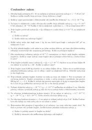
Contents General remarks <strong>The</strong> “classical” region Tunneling <strong>The</strong> connection formulas LiteratureExample: Gamow’s theory of alpha decayfirst time that quantum<strong>mechanics</strong> had beenapplied to nuclearphysicsIgor Lukačević<strong>The</strong> <strong>WKB</strong> <strong>approximation</strong>UJJS, Dept. of Physics, Osijek
Contents General remarks <strong>The</strong> “classical” region Tunneling <strong>The</strong> connection formulas LiteratureExample: Gamow’s theory of alpha decay (cont.)first time that quantum<strong>mechanics</strong> had beenapplied to nuclearphysicsturning points:1 r 1 ↦−→ nucleus radius(6.63 fm for U 238 )2 r 2 ↦−→1 2Ze 2= E4πɛ 0 r 2Igor Lukačević<strong>The</strong> <strong>WKB</strong> <strong>approximation</strong>UJJS, Dept. of Physics, Osijek
Contents General remarks <strong>The</strong> “classical” region Tunneling <strong>The</strong> connection formulas LiteratureExample: Gamow’s theory of alpha decay (cont.)γ = 1 ∫√r2( ) √ ∫ 1 2Ze2m22mE r2√r2− E dr = r 14πɛ 0 r 2 r 1r − 1drIgor Lukačević<strong>The</strong> <strong>WKB</strong> <strong>approximation</strong>UJJS, Dept. of Physics, Osijek
Contents General remarks <strong>The</strong> “classical” region Tunneling <strong>The</strong> connection formulas LiteratureExample: Gamow’s theory of alpha decay (cont.)γ = 1 ∫√r2( ) √ ∫ 1 2Ze2m22mE r2√r2− E dr = r 14πɛ 0 r 2 r 1r − 1drSubstituting r = r 2 sin 2 u gives√ [ ( √ )2mE πγ = r 2 2 − r1sin−1 − √ ]r 1(r 2 − r 1)r 2Igor Lukačević<strong>The</strong> <strong>WKB</strong> <strong>approximation</strong>UJJS, Dept. of Physics, Osijek
Contents General remarks <strong>The</strong> “classical” region Tunneling <strong>The</strong> connection formulas LiteratureExample: Gamow’s theory of alpha decay (cont.)γ = 1 ∫√r2( ) √ ∫ 1 2Ze2m22mE r2√r2− E dr = r 14πɛ 0 r 2 r 1r − 1drSubstituting r = r 2 sin 2 u gives√ { [ √ ]2mE πγ = r 2 2 − r1sin−1 − √ }r 1(r 2 − r 1)r 2 } {{ }} {{ } √r 1 ≪r−−−→2 √ r1 r 2 −r 2 r 1 ≪r1 −−−→2 √ r1 r 2r1 /r 2} {{ }π2r 2 −2 √ r 1 r 2Igor Lukačević<strong>The</strong> <strong>WKB</strong> <strong>approximation</strong>UJJS, Dept. of Physics, Osijek
Contents General remarks <strong>The</strong> “classical” region Tunneling <strong>The</strong> connection formulas LiteratureExample: Gamow’s theory of alpha decay (cont.)Substituting r = r 2 sin 2 u gives√ { [ √ ]2mE πγ = r 2 2 − r1sin−1 − √ }r 1(r 2 − r 1)r 2 } {{ }} {{ } √r 1 ≪r−−−→2 √ r1 r 2 −r 2 r 1 ≪r1 −−−→2 √ r1 r 2r1 /r 2} {{ }π2r 2 −2 √ r 1 r 2where√2mE[ π]γ ≈ 2 r2 − 2√ Z √r 1r 2 = K 1 √E − K 2 Zr1K 1 =K 2 =( ) √e2 π 2m= 1.980 MeV 1/24πɛ 0 ( ) e2 1/2 √ 4 m= 1.485 fm −1/24πɛ 0 Igor Lukačević<strong>The</strong> <strong>WKB</strong> <strong>approximation</strong>UJJS, Dept. of Physics, Osijek
Contents General remarks <strong>The</strong> “classical” region Tunneling <strong>The</strong> connection formulas LiteratureExample: Gamow’s theory of alpha decay (cont.)v average velocity2r 1/v average timebetween “collisions”with the nucleuspotential “wall”v/2r 1 averagefrequancy of “collisions”e −2γ “escape”probability(v/2r 1)e −2γ “escape” probability perunit timeLifetime:τ = 2r1v e2γIgor Lukačević<strong>The</strong> <strong>WKB</strong> <strong>approximation</strong>UJJS, Dept. of Physics, Osijek
Contents General remarks <strong>The</strong> “classical” region Tunneling <strong>The</strong> connection formulas LiteratureExample: Gamow’s theory of alpha decay (cont.)v average velocity2r 1/v average timebetween “collisions”with the nucleuspotential “wall”v/2r 1 averagefrequancy of “collisions”e −2γ “escape”probability(v/2r 1)e −2γ “escape” probability perunit timeLifetime:τ = 2r1v e2γ ⇒ ln τ ∼ 1 √EIgor Lukačević<strong>The</strong> <strong>WKB</strong> <strong>approximation</strong>UJJS, Dept. of Physics, Osijek
Contents General remarks <strong>The</strong> “classical” region Tunneling <strong>The</strong> connection formulas LiteratureHWSolve Problem 8.3 from Ref. [2].Igor Lukačević<strong>The</strong> <strong>WKB</strong> <strong>approximation</strong>UJJS, Dept. of Physics, Osijek
Contents General remarks <strong>The</strong> “classical” region Tunneling <strong>The</strong> connection formulas LiteratureContents1 General remarks2 <strong>The</strong> “classical” region3 Tunneling4 <strong>The</strong> connection formulas5 LiteratureIgor Lukačević<strong>The</strong> <strong>WKB</strong> <strong>approximation</strong>UJJS, Dept. of Physics, Osijek
Contents General remarks <strong>The</strong> “classical” region Tunneling <strong>The</strong> connection formulas LiteratureIgor Lukačević<strong>The</strong> <strong>WKB</strong> <strong>approximation</strong>UJJS, Dept. of Physics, Osijek
Contents General remarks <strong>The</strong> “classical” region Tunneling <strong>The</strong> connection formulas LiteratureLet us repeat:⎧⎨ψ(x) ≈⎩√1[Be i ∫ 0 x p(x ′ )dx ′ + Ce − i ∫ 0p(x)√1De − 1p(x)x p(x ′ )dx ′] , if x < 0∫ x0|p(x ′ )|dx ′ , if x > 0Igor Lukačević<strong>The</strong> <strong>WKB</strong> <strong>approximation</strong>UJJS, Dept. of Physics, Osijek
Contents General remarks <strong>The</strong> “classical” region Tunneling <strong>The</strong> connection formulas LiteratureLet us repeat:⎧⎨ψ(x) ≈⎩√1[Be i ∫ 0 x p(x ′ )dx ′ + Ce − i ∫ 0p(x)√1De − 1p(x)x p(x ′ )dx ′] , if x < 0∫ x0|p(x ′ )|dx ′ , if x > 0Our mission: join these two solutions at the boundary.Igor Lukačević<strong>The</strong> <strong>WKB</strong> <strong>approximation</strong>UJJS, Dept. of Physics, Osijek
Contents General remarks <strong>The</strong> “classical” region Tunneling <strong>The</strong> connection formulas LiteratureLet us repeat:⎧⎨ψ(x) ≈⎩√1[Be i ∫ 0 x p(x ′ )dx ′ + Ce − i ∫ 0p(x)√1De − 1p(x)x p(x ′ )dx ′] , if x < 0∫ x0|p(x ′ )|dx ′ , if x > 0Our mission: join these two solutions at the boundary.A problemWhat happens with the w.f. whenE ≈ V ?Igor Lukačević<strong>The</strong> <strong>WKB</strong> <strong>approximation</strong>UJJS, Dept. of Physics, Osijek
Contents General remarks <strong>The</strong> “classical” region Tunneling <strong>The</strong> connection formulas LiteratureLet us repeat:⎧⎨ψ(x) ≈⎩√1[Be i ∫ 0 x p(x ′ )dx ′ + Ce − i ∫ 0p(x)√1De − 1p(x)x p(x ′ )dx ′] , if x < 0∫ x0|p(x ′ )|dx ′ , if x > 0Our mission: join these two solutions at the boundary.A problemWhat happens with the w.f. whenE ≈ V ?E ≈ V ⇒ p(x) → 0 ⇒ ψ → ∞ !Igor Lukačević<strong>The</strong> <strong>WKB</strong> <strong>approximation</strong>UJJS, Dept. of Physics, Osijek
Contents General remarks <strong>The</strong> “classical” region Tunneling <strong>The</strong> connection formulas LiteratureLet us repeat:⎧⎨ψ(x) ≈⎩√1[Be i ∫ 0 x p(x ′ )dx ′ + Ce − i ∫ 0p(x)√1De − 1p(x)x p(x ′ )dx ′] , if x < 0∫ x0|p(x ′ )|dx ′ , if x > 0Our mission: join these two solutions at the boundary.A problemWhat happens with the w.f. whenE ≈ V ?E ≈ V ⇒ p(x) → 0 ⇒ ψ → ∞ !A solutionConstruct a “patching”wavefunction ψ p.Igor Lukačević<strong>The</strong> <strong>WKB</strong> <strong>approximation</strong>UJJS, Dept. of Physics, Osijek
Contents General remarks <strong>The</strong> “classical” region Tunneling <strong>The</strong> connection formulas LiteratureApproximation: we linearize the potentialV (x) ≈ E + V ′ (0)xIgor Lukačević<strong>The</strong> <strong>WKB</strong> <strong>approximation</strong>UJJS, Dept. of Physics, Osijek
Contents General remarks <strong>The</strong> “classical” region Tunneling <strong>The</strong> connection formulas LiteratureApproximation: we linearize the potentialFrom S.E. we get V (x) ≈ E + V ′ (0)x[ ]d 2 1ψ p2m= zψdz 2 p , z = αx , α = V ′ 3(0)2Igor Lukačević<strong>The</strong> <strong>WKB</strong> <strong>approximation</strong>UJJS, Dept. of Physics, Osijek
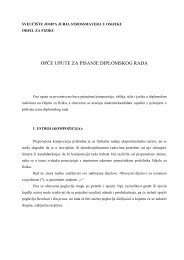
Contents General remarks <strong>The</strong> “classical” region Tunneling <strong>The</strong> connection formulas LiteratureApproximation: we linearize the potentialFrom S.E. we get V (x) ≈ E + V ′ (0)xd 2 ψ p= zψdz 2 p ,} {{ }z = αx , α =Airy’s equation[ ] 12m V ′ 3(0)2Igor Lukačević<strong>The</strong> <strong>WKB</strong> <strong>approximation</strong>UJJS, Dept. of Physics, Osijek
Contents General remarks <strong>The</strong> “classical” region Tunneling <strong>The</strong> connection formulas LiteratureApproximation: we linearize the potentialFrom S.E. we get V (x) ≈ E + V ′ (0)xd 2 ψ p= zψdz 2 p ,} {{ }z = αx , α =Airy’s equation[ ] 12m V ′ 3(0)2ψ p = a Ai(αx)} {{ }+b Bi(αx)} {{ }Airy function Airy functionIgor Lukačević<strong>The</strong> <strong>WKB</strong> <strong>approximation</strong>UJJS, Dept. of Physics, Osijek
Contents General remarks <strong>The</strong> “classical” region Tunneling <strong>The</strong> connection formulas LiteratureIgor Lukačević<strong>The</strong> <strong>WKB</strong> <strong>approximation</strong>UJJS, Dept. of Physics, Osijek
Contents General remarks <strong>The</strong> “classical” region Tunneling <strong>The</strong> connection formulas Literaturea delicate double constraint has to be satisfiedIgor Lukačević<strong>The</strong> <strong>WKB</strong> <strong>approximation</strong>UJJS, Dept. of Physics, Osijek
Contents General remarks <strong>The</strong> “classical” region Tunneling <strong>The</strong> connection formulas Literaturea delicate double constraint has to be satisfiedwe need <strong>WKB</strong> w.f. and ψ p for both overlap regions (OLR)Igor Lukačević<strong>The</strong> <strong>WKB</strong> <strong>approximation</strong>UJJS, Dept. of Physics, Osijek
Contents General remarks <strong>The</strong> “classical” region Tunneling <strong>The</strong> connection formulas Literaturep(x) = √ 2m(E − V ) ≈ α 3 2√−xIgor Lukačević<strong>The</strong> <strong>WKB</strong> <strong>approximation</strong>UJJS, Dept. of Physics, Osijek
Contents General remarks <strong>The</strong> “classical” region Tunneling <strong>The</strong> connection formulas Literaturep(x) ≈ α 3 √2 −xOLR 2 (x > 0)∫ x0|p(x ′ )|dx ′ ≈ 2 3 (αx) 3 2ψ <strong>WKB</strong>ψ z≫0p≈≈D√α3/4x 1/4 e− 2 3 (αx)3/2a2 √ π(αx) 1/4 e− 2 3 (αx)3/2b+ √ e 3 2 (αx)3/2π(αx)1/4⇒ a = D√4πα , b = 0Igor Lukačević<strong>The</strong> <strong>WKB</strong> <strong>approximation</strong>UJJS, Dept. of Physics, Osijek
Contents General remarks <strong>The</strong> “classical” region Tunneling <strong>The</strong> connection formulas LiteratureOLR 2 (x > 0)∫ x0ψ <strong>WKB</strong>ψ z≫0p√4πα , b = 0 OLR 1 (x < 0)|p(x ′ )|dx ′ ≈ 2 ∫3 (αx) 3 02xD√ 2 α3/4x 1/4 e− 3 (αx)3/2ψ <strong>WKB</strong> ≈a2 √ 2 π(αx) 1/4 e− 3 (αx)3/2b+ √ e 3 2 (αx)3/2 ψ z≪0π(αx)1/4 p ≈≈≈⇒ a = D⇒p(x ′ )dx ′ ≈ 2 3 (−αx) 3 21[√ Be i 2 3 (−αx)3/2α3/4(−x) 1/4+Ce −i 2 3 (−αx)3/2]a 1√ π(−αx)1/4 2i−e −iπ/4 e −i 2 3 (−αx)3/2]a2i √ π eiπ/4 = √ Bα−a2i √ π e−iπ/4 = √ Cα[e iπ/4 e i 2 3 (−αx)3/2Igor Lukačević<strong>The</strong> <strong>WKB</strong> <strong>approximation</strong>UJJS, Dept. of Physics, Osijek
Contents General remarks <strong>The</strong> “classical” region Tunneling <strong>The</strong> connection formulas Literature<strong>The</strong> connection formulasB = −ie iπ/4 · D ,C = ie −iπ/4 · DIgor Lukačević<strong>The</strong> <strong>WKB</strong> <strong>approximation</strong>UJJS, Dept. of Physics, Osijek
Contents General remarks <strong>The</strong> “classical” region Tunneling <strong>The</strong> connection formulas Literature<strong>The</strong> connection formulasB = −ie iπ/4 · D ,C = ie −iπ/4 · D<strong>WKB</strong> w.f.⎧⎪⎨ψ(x) ≈⎪⎩[ ∫2D 1 x2√ sin p(x ′ )dx ′ + π ], if x < x 2p(x) x4[D√ exp − 1 ∫ x]|p(x ′ )|dx ′ , if x > x 2|p(x)| x 2Igor Lukačević<strong>The</strong> <strong>WKB</strong> <strong>approximation</strong>UJJS, Dept. of Physics, Osijek
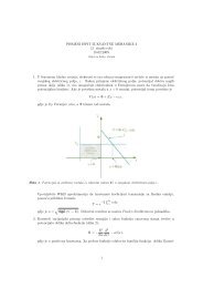
Contents General remarks <strong>The</strong> “classical” region Tunneling <strong>The</strong> connection formulas LiteratureExample: Potentail well with one vertical wallIgor Lukačević<strong>The</strong> <strong>WKB</strong> <strong>approximation</strong>UJJS, Dept. of Physics, Osijek
Contents General remarks <strong>The</strong> “classical” region Tunneling <strong>The</strong> connection formulas LiteratureExample: Potentail well with one vertical wallBoundary condition: ψ(0) = 0, gives for ψ <strong>WKB</strong>∫ x2(p(x)dx = n − 1 )π , n = 1, 2, 3, . . .40Igor Lukačević<strong>The</strong> <strong>WKB</strong> <strong>approximation</strong>UJJS, Dept. of Physics, Osijek
Contents General remarks <strong>The</strong> “classical” region Tunneling <strong>The</strong> connection formulas LiteratureExample: Potentail well with one vertical wall (cont.)For instance, consider the “half-harmonic oscillator”:⎧1 ⎪⎨V (x) =2 mω2 x 2 , x > 0⎪⎩0 otherwiseIgor Lukačević<strong>The</strong> <strong>WKB</strong> <strong>approximation</strong>UJJS, Dept. of Physics, Osijek
Contents General remarks <strong>The</strong> “classical” region Tunneling <strong>The</strong> connection formulas LiteratureExample: Potentail well with one vertical wall (cont.)For instance, consider the “half-harmonic oscillator”:⎧1 ⎪⎨V (x) =2 mω2 x 2 , x > 0⎪⎩0 otherwiseHere we have√p(x) = mω x2 2 − x 2Igor Lukačević<strong>The</strong> <strong>WKB</strong> <strong>approximation</strong>UJJS, Dept. of Physics, Osijek
Contents General remarks <strong>The</strong> “classical” region Tunneling <strong>The</strong> connection formulas LiteratureExample: Potentail well with one vertical wall (cont.)For instance, consider the “half-harmonic oscillator”:⎧1 ⎪⎨V (x) =2 mω2 x 2 , x > 0⎪⎩0 otherwiseHere we haveSo√p(x) = mω x2 2 − x 2∫ x20p(x)dx = πE2ωIgor Lukačević<strong>The</strong> <strong>WKB</strong> <strong>approximation</strong>UJJS, Dept. of Physics, Osijek
Contents General remarks <strong>The</strong> “classical” region Tunneling <strong>The</strong> connection formulas LiteratureExample: Potentail well with one vertical wall (cont.)For instance, consider the “half-harmonic oscillator”:⎧1 ⎪⎨V (x) =2 mω2 x 2 , x > 0⎪⎩0 otherwiseHere we haveSoComparisson now gives:E n =√p(x) = mω x2 2 − x 2∫ x20p(x)dx = πE2ω(2n − 1 ) ( 3ω =2 2 , 7 2 , 11 )2 , . . . ωIgor Lukačević<strong>The</strong> <strong>WKB</strong> <strong>approximation</strong>UJJS, Dept. of Physics, Osijek
Contents General remarks <strong>The</strong> “classical” region Tunneling <strong>The</strong> connection formulas LiteratureExample: Potentail well with one vertical wall (cont.)For instance, consider the “half-harmonic oscillator”:⎧1 ⎪⎨V (x) =2 mω2 x 2 , x > 0⎪⎩0 otherwiseHere we haveSoComparisson now gives:E n =√p(x) = mω x2 2 − x 2∫ x2Compare this result with an exact one.0p(x)dx = πE2ω(2n − 1 ) ( 3ω =2 2 , 7 2 , 11 )2 , . . . ωIgor Lukačević<strong>The</strong> <strong>WKB</strong> <strong>approximation</strong>UJJS, Dept. of Physics, Osijek
Contents General remarks <strong>The</strong> “classical” region Tunneling <strong>The</strong> connection formulas LiteratureExample: Potential well with no vertical wallsIgor Lukačević<strong>The</strong> <strong>WKB</strong> <strong>approximation</strong>UJJS, Dept. of Physics, Osijek
Contents General remarks <strong>The</strong> “classical” region Tunneling <strong>The</strong> connection formulas LiteratureExample: Potential well with no vertical wallswe have seen the connection formulas for upward potential slopesfor downward slopes (analogous):⎧D ′√ exp|p(x)|⎪⎨ψ(x) ≈⎪⎩[− 1 ∫ x1x]|p(x ′ )|dx ′ , if x < x 1[2D ′ ∫ 1 x√ sin p(x ′ )dx ′ + π ], if x > x 1p(x) x 14Igor Lukačević<strong>The</strong> <strong>WKB</strong> <strong>approximation</strong>UJJS, Dept. of Physics, Osijek
Contents General remarks <strong>The</strong> “classical” region Tunneling <strong>The</strong> connection formulas LiteratureExample: Potential well with no vertical wallswe want the w.f. in the “well”, i.e. where x 1 < x < x 2:ψ(x) ≈2D √p(x)sin θ 2(x) ,ψ(x) ≈ − 2D′ √p(x)sin θ 1(x) ,θ 2(x) = 1 θ 1(x) = − 1 ∫ x2x∫ xp(x ′ )dx ′ + π 4x 1p(x ′ )dx ′ − π 4Igor Lukačević<strong>The</strong> <strong>WKB</strong> <strong>approximation</strong>UJJS, Dept. of Physics, Osijek
Contents General remarks <strong>The</strong> “classical” region Tunneling <strong>The</strong> connection formulas LiteratureExample: Potential well with no vertical wallssin θ 1 = sin θ 2 =⇒ θ 2 = θ 1 + nπ =⇒∫ x2(p(x)dx = n − 1 )π , n = 1, 2, 3, . . .x 12Igor Lukačević<strong>The</strong> <strong>WKB</strong> <strong>approximation</strong>UJJS, Dept. of Physics, Osijek
Contents General remarks <strong>The</strong> “classical” region Tunneling <strong>The</strong> connection formulas LiteratureExample: Potential well with no vertical wallssin θ 1 = sin θ 2 =⇒ θ 2 = θ 1 + nπ =⇒∫ x2(p(x)dx = n − 1 )π , n = 1, 2, 3, . . .x 12 0, two vertical walls 1/4, one vertical wallIgor Lukačević<strong>The</strong> <strong>WKB</strong> <strong>approximation</strong>UJJS, Dept. of Physics, Osijek
Contents General remarks <strong>The</strong> “classical” region Tunneling <strong>The</strong> connection formulas LiteratureConclusions<strong>WKB</strong> advantagesgood for slowly changing w.f.good for short wavelengthsbest in the semi-classicalsystems (large n)one doesn’t even have to solvethe S.E.<strong>WKB</strong> disadvantagesbad for rapidly changing w.f.bad for long wavelengthsinappropriate for lower states(small n)constraint trade-off (sometimesnot possible)Igor Lukačević<strong>The</strong> <strong>WKB</strong> <strong>approximation</strong>UJJS, Dept. of Physics, Osijek
Contents General remarks <strong>The</strong> “classical” region Tunneling <strong>The</strong> connection formulas LiteratureContents1 General remarks2 <strong>The</strong> “classical” region3 Tunneling4 <strong>The</strong> connection formulas5 LiteratureIgor Lukačević<strong>The</strong> <strong>WKB</strong> <strong>approximation</strong>UJJS, Dept. of Physics, Osijek
Contents General remarks <strong>The</strong> “classical” region Tunneling <strong>The</strong> connection formulas LiteratureLiterature1 R. L. Liboff, Introductory <strong>Quantum</strong> Mechanics, Addison Wesley, SanFrancisco, 2003.2 D. J. Griffiths, Introduction to <strong>Quantum</strong> Mechanics, 2nd ed., PearsonEducation, Inc., Upper Saddle River, NJ, 2005.3 I. Supek, Teorijska fizika i struktura materije, II. dio, Školska knjiga,Zagreb, 1989.4 Y. Peleg, R. Pnini, E. Zaarur, Shaum’s Outline of <strong>The</strong>ory and Problems of<strong>Quantum</strong> Mechanics, McGraw-Hill, 1998.Igor Lukačević<strong>The</strong> <strong>WKB</strong> <strong>approximation</strong>UJJS, Dept. of Physics, Osijek