V - Esigelec

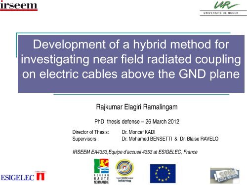
Development of a hybrid method forinvestigating near field radiated couplingon electric cables above the GND planeRajkumar Elagiri RamalingamPhD thesis defense – 26 March 2012Director of Thesis:Supervisors :Dr. Moncef KADIDr. Mohamed BENSETTI & Dr. Blaise RAVELOIRSEEM EA4353,Equipe d’accueil 4353 at ESIGELEC, France

Outline• General introduction• Methodology of the electric wire radiated coupling modeling withHybrid Method (HM)• Experimental validations of HM for cables susceptibility in widefrequency band• Application of HM for the modelling of near-field (NF) agression oncomplex form metallic wires• Conclusions and perspectives2

Outline• General introduction• Motivation• Thesis Objective & Work Flow• State of the art of the existing NF coupling modeling• Summary• Methodology of the electric wire radiated coupling modeling withHybrid Method (HM)• Experimental validations of HM for cables susceptibility in widefrequency band• Application of HM for the modelling of near-field (NF) agression oncomplex form metallic wires• Conclusions and perspectives3

Thesis objective & Work flow (TECS-WP5)RadiatedFieldRadiating componentRadiated Emissionmodels –Group 1Network ofDipolesNF coupling test - cableRadiated ImmunityModels –GroupDevelopment of methodology for NF coupling between components and cables1. Y.-G. Vives, Ph.D Thesis, IRSEEM, Univ. Rouen, 2007TECS-INTERREG IV A –WP55

Radiated Emission ModelRadiated FieldDevice under testElectric dipole array∆l∆lI 1 ,θ 1∆l∆lI 2 ,θ 2I 3 ,θ 3 I 4 ,θ 4Model based on a set of electric andmagnetic dipoles placed on a XY-plane 1 .Parameters fixed by the user:- Number- Length- Position1. P.F-Lopez ,Ph.D Thesis, IRSEEM, Univ. Rouen, 2011Characteristics• The dipole array radiates the same EM fieldas that of the DUT• Generic model – can be applied to anycomponent• Parametric extraction based on the use ofan iterative algorithm.• Model validated on a variety of componentsin a wide frequency range.• Simple and robust in its implementation• Easily integrable into commercial EM tools.6

Coupling modelIncidentfields (E i , H i )+Reflectedfields (E r , H r )=Excitingfields (E e , H e )E excitation = E incident +• Obtaining an expression for the voltage and current induced in the line due to an EMdisturbance+EreflectedTelegrapher’s equationsExcitation sources7

Radiated immunityDifferent analytical models:Taylor model: Modeling with E- & H-fieldAgrawal model: Modeling only with E-fieldRachidi model : Model only with H-field8

Taylor modelTaylor model: Model with Magnetic & Electric components of field 1Equations:dI(x)+dx'jwC VdV ( x)'+ jwL I(x)= − jwµ0dx' e( x) = − jwC E ( x,z)dzh∫0h∫0Hzey( x,z)dzBoundary's Conditions :V ( 0) = −ZI(0)AV ( L)= Z I(L)BL' dxVs1ZAV(0)V(x)Is1C' dxV(x+dx)V(L)ZB1.C. D. Taylor et al, IEEE Trans. Ant. Prop., vol. E, 1965.0 xx+dx LEquivalent “Taylor model” circuit Complex numerical resolution9

Agrawal modelAgrawal model: Model with only electrical components of field 1Agrawal Model :Equations:esV ( x)= V ( x)+ V ( x)= −∫EsdV ( x)'e+ jwLI(x)= Ex( x,h)dxdI( x)' s+ jwC V ( x)= 0dxh0e( x,z)dz + Vs( x)VSV(0) = −ZSBoundary's Conditions :( L)= ZABhI(0)+ ∫ E0hI(L)+ ∫ E0ezeZ(0, z)dz( L,z)dzL' dxV S (0)V(x)C' dxV(x+dx)V S (L)ZAZB0 xx+dx L1.A. K. Agrawal et al, IEEE Trans. Ant. and Prop., vol. 18, 1980.Equivalent “Agrawal model” circuit Simple numerical resolution10

Rachidi modelRachidi Model :Equations:Rachidi model : Model with only Magnetic components of field 1dV ( x)' s+ jwLI ( x)= 0dxsdI ( x)µ0+ jwC V ( x)=dxLIe s s( x) = I ( x) + I ( x) = I ( x) − ∫h' )∫0e∂Hx( x,z∂ydzhe0Hy( x,z)'01 µLdzIsIsBoundary's Conditions :V (0) µ0(0) = − +Z LV ( L)µ0( L)= − +Z LBAh∫0h∫0HHeyey(0, z)dz( L,z)dzZAV S (0)V(x)L' dx1Is4C' dxV(x+dx)V S (L)ZBIs6Is51.F. Rachidi, IEEE Trans EMC, vol. 35, 19930 xx+dx LEquivalent “Rachidi model” circuitComplex numerical resolution11

Comparison of coupling modelsComparison between different analytical methods:Model Electric field Magnetic field DevelopedAnalyticalresolution 1,2Taylor Ez Hy YesAgrawal Ex, Ez - YesRachidi - Hx, Hz -1. S.Atrous ,Ph.D Thesis, IRSEEM, Univ. Rouen, 2009 2.C.Leseigneur,Ph.D Thesis, IRSEEM, Univ. Rouen, 201012

Dipole model To validate the electric dipole Ex and Ez components 1Ez= 60⋅I0⋅dl⋅e− jkR⎡⎛2⋅⎢⎜⋅ ⎢⎝⎢⎢ jk−⎢⎣2R2( z − z ) − ( x − x )0R( x − x )220302Elementary electric dipole⎞ ⎛ 1⎟⋅⎜⎠ ⎝ 2R21+2 jkR3⎞⎤⎟⎥⎠⎥⎥⎥⎥⎦E= 30⋅I⋅dl⋅⎡⎢⎣r− jkRe 3 3 ⎤( z − z ) ⋅( x − x ) ⋅ ⋅ + + jk⎥ ⎦x 000 32Rjkr1.P.Fernandez-lopez, Ph.D Thesis,IRSEEM,Univ.Rouen Jan. 201113

Implementation -Dipole ModelCharacteristics of the Dipole:Current = 0.2 A DipoleLength = 1 mmRadius = 0.1 mmFrequency = 2 GHzZ -component field is computed across the integration lineHFSS design of dipole model implementationf=2GHz2000TheoryHFSSFEMAnalytical Method|E z| V/m1500100050000 0.1 0.2 0.3 0.4 0.5 0.6 0.7 0.8 0.9Diatance (mm)V 1 V 2 V 1 V 21.7836 1.7858 1.8413 1.8413The relative error is less than 2%14

Analytical Model-Flow summaryStartDefinition of systemCable with Perturbation source to be definedCalculation of the EM wave excitations E and Hwithout the victim system 1Determination of the field in the presence of theground plane by Image theoryExtraction of total field neglecting scattering fieldCalculation of Induced voltageStop1.C.Leseigneur,Ph.D Thesis, IRSEEM, Univ. Rouen, 201015

Application: dipole placed between ground plane and cableCableCableLength = 8 mmRadius = 0.1 mmDipole221 Ω 221 ΩGround PlaneLength = 28 mmWidth = 20 mmThickness = 0.2 mmGround PlaneDipoleCurrent = 0.2 ALength = 1 mmwidth = 0.1 mmCharacteristicImpedance−1Z c=12πµ 0coshε0⎛ h ⎞⎜ ⎟⎝ a ⎠Cable-Ground planeCapacitance unitlengthC0=2πε0⎛ 2hln⎜⎝ a⎞⎟⎠Z0 = ZL= Zc= 221ΩInductance perunit lengthµ 0 ⎛ 2dL u = ln⎜ 2π⎝ a⎟⎠⎞16

Analytical Model ResultsAnalytical model comparison with FEMDipole placed at 2mm above cableAnalytical results are not in good accordance with FEM17

Analytical Model ResultsAnalytical model comparison with FEMDipole placed at 1mm above cable• Analytical results are not in good accordance with FEM18

Analytical Model ResultsAnalytical model comparison with FEMDipole placed at 1mm below cableAnalytical results are not in good accordance with FEM19

Summary-Limitations of existing methods• Existing models are not valid for perturbation source near the cable• It is not considering all the coupling phenomena’s• Very suitable for far field analysis20

Outline• General introduction• Methodology of the electric wire radiated coupling modeling withHybrid Method (HM)• Need• Flow chart & Formulation• Implementation of HM• Results- comparison• Advantages and Summary• Experimental validations of HM for cables susceptibility in widefrequency band• Application of HM for the modelling of near-field (NF) agression oncomplex form metallic wires• Conclusions and perspectives21

HM-Need Proposed HM is to be capable To overcome the technical limitationsWhen the dipole is near to the line, this should give good voltage accuracy The coupling model does take into account of the mutual coupling: betweenthe cable and ground planethe dipole and cablethe dipole and ground plane.22

HM Model-Flow summaryStartDefinition of system understudy:Cable with Perturbation sourceCalculation of the EM wave excitations E and Hwith the victim systemDetermination of the field in the presence of cableand ground planeExtraction of Total field including scattering field(simulation/measurement)Calculation of Induced voltageStopE.R.Rajkumar et al ,PIER B 37, pp. 143-169, 2012.23

HM - Procedure• Victim and perturbation source to be defined• Configuration and parameters of both to be clearly defined• Choice of HM• Electric and magnetic fields to be extracted by calculation /measurement• Integration of extracted fields to obtained the current and voltage sources• Calculation of the voltage in the loads24

HM based on the Agrawal modelCableCableLength = 8 mmRadius = 0.1 mmDipole221 Ω 221 ΩGround PlaneLength = 28 mmWidth = 20 mmThickness = 0.2 mmGround PlaneDipoleCurrent = 0.2 ALength = 1 mmWidth = 0.1 mmy V(y)yV(0)V(L)Tesche et al, 200425

HM – implementationFormulation in frequency domain:y V(y)yV(0)V(L)L⎡ 1 y V1 V ⎤γ2 γL−1e Vs( y)dy eγ L⎢− + ⎥V (0) 1+ρ2 2 210 ⎡ ρ1e ⎤∫⎡ ⎤ ⎡⎤ − ⎢ 0⎥⎢ LLV( L) ⎥ = ⎢γ0 1 ρ⎥⎢ ⎥2 e ρ ⎢2 1 γ( L−y) V1 γLV⎥⎣ ⎦ ⎣ + ⎦⎣ − ⎦ ⎢2− e Vs( y)dy + e − ⎥⎢ 2∫⎣2 20⎥⎦Vh= −∫1Ez0, z)0h( dz V = −∫E2 zL,z)0( dz V( y) = E ( yh , )syTesche et al, 200426

HM – implementation1- Determination of the total electric field in the absence of the loadsCablezE zOpen1.9 mmDipoleEyOpenE zyGround PlaneHFSS simulation - for building Hybrid (Agrawal’s) model .2- Extraction of the E z and E y component and elimination the reflection problem by interpolation|Ey|(KV/m)Reflection dueto absence ofloady(mm)Reflection dueto absence ofloadE. R. Rajkumar et al, workshop 2emc 2010, Rouen, France, 18-19 Nov. 201027

HM – implementation3- Calculation of V 1, V 2 and V s by using the following equations:Vh= −∫1Ez0, z)0h( dz V = −∫E2 z, )0( L z dz V( y) = E ( yh , )V s : Depending on the total longitudinal electric field (E y )V 1 and V 2 : Depending on the total transversal electric field (E Z )4- Determination the induced voltage between the loads by using the following equations:L⎡ 1 y V1 V ⎤γ2 γL−1e Vs( y)dy eγ L⎢− + ⎥V (0) 1+ρ2 2 210 ⎡ ρ1e ⎤∫⎡ ⎤ ⎡⎤ − ⎢ 0⎥⎢ LLV( L) ⎥ = ⎢γ0 1 ρ⎥⎢ ⎥2 e ρ ⎢2 1 γ( L−y) V1 γLV⎥⎣ ⎦ ⎣ + ⎦⎣ − ⎦ ⎢2− e Vs( y)dy + e − ⎥⎢ 2∫⎣2 20⎥⎦ρ 1Z=Zaa−+ZZccρ 2sZ=Zbb− Z+ ZccyE. R. Rajkumar et al, workshop 2emc 2010, Rouen, France, 18-19 Nov. 201028

HM based on the Taylor modelCableCableLength = 8 mmRadius = 0.1 mmElectrical model:221 Ω 221 ΩDipoleGround PlaneLength = 28 mmWidth = 20 mmThickness = 0.2 mmGround PlaneDipoleCurrent = 0.2 ALength = 1 mmWidth = 0.1 mm1.E.R.Rajkumar et al, PIERS, Marrakech, Morocco, 20-23 March, 2011.29

HM –FormulationFormulation in frequency domain:1- Determination of the total electric and magnetic fields in the center of element mesh in the absence of the loadsArea of interest2. Calculation of the voltage and current sources by the following formulations:I ( jω)⋅ L = −jω⋅C ⋅A⋅Es u zV ( jω)⋅ L = −j ω⋅µ ⋅A⋅Hs0yA =area between the line and ground planeL = length of the cableh=height of cable from ground planeE.R.Rajkumar et al, PIERS, Marrakech, Morocco, 20-23 March, 2011.30

HM –Formulation3- Calculation the voltage on the loads by using the following expressions:ZZZLV(0)= V ⋅L− Is⋅LZ + Z Z + Z0 0s0 L0LZZZLV( L)= − V ⋅L− Is⋅LZ + Z Z + Z0 0s0 L0L31

HM(Agrawal)ResultsDipole placed at 1mm below cable2.52.52HFSSHybridAgrawal2HFSSHybridAgrawal1.51.5V(0) (V)1V(L) (V)10.50.500 0.5 1 1.5 2Freq (GHz)00 0.5 1 1.5 2Freq (GHz)• Good correlation between FEM and HM• The relative error is less than 3 %32

HM(Agrawal)ResultsDipole placed at 3mm above cable776.5HFSSHybridAgrawal6.5HFSSHybridAgrawal66V(0)5.5V(L)5.5554.54.540 0.5 1 1.5 2Freq (GHz)40 0.5 1 1.5 2Freq (GHz)• Good correlation between FEM and HM• The relative error is less than 2%33

HM(Taylor)ResultsDipole placed at 1mm below cable54.5HFSSHybrid(Taylor)54.5HFSSHybrid(Taylor)443.53.533V(0) (V)2.5V(L) (V)2.5221.51.5110.50.500 0.5 1 1.5 2Freq (GHz)00 0.5 1 1.5 2Freq (GHz)• Good correlation between FEM and HM• The relative error is less than 4%34

HM(Taylor)ResultsDipole placed at 3mm above cable776.56.56HFSSHybridTaylor6HFSSHybridTaylorV(0)5.5V(L)5.5554.54.540 0.5 1 1.5 2Freq (GHz)40 0.5 1 1.5 2Freq (GHz)• Good correlation between FEM and HM• The relative error is less than 5%35

HM-Advantages & SummaryHM is calculated in the presence of the cableScattering effect is also consideredValidated for various positions of dipole sourceHM is considering all mutual coupling between the source and thevictimHM is capable of handling industrial real time situations36

Outline• General introduction• Methodology of the electric wire radiated coupling modeling withHybrid Method (HM)• Experimental validations of HM for cables susceptibility in widefrequency bandDescription of configurationExperiments by using two cablesExperiments with patch antennaSummary• Application of HM for the modelling of near-field (NF) agression oncomplex form metallic wires• Conclusions and perspectives37

Experimental Validation: coupling between two cablesDescription of the problem: study the coupling between two cablesVictim cablePerturbation sourceCablesconfiguration:Length=d 1 =d 2 =30mmr =0.5mmh=20mmZ 0 =200ΩDifferent studies:1- Study the coupling by HM ( the effect of the victim cable is considered)2- Source and victim are parallel and perpendicular38

Validation-Flow chartE.R.Rajkumar et al ,IJAET, Paper ID: IJAET0703711, May 201239

Validation –Experimental setupMeasurement-Near field test benchAmplifierPowerGeneratorNETWORKANALYZERDUTE.R.Rajkumar et al ,IJAET, Paper ID: IJAET0703711, May 201240

Validation –Experimental setupMeasurement-NF test benchFrequency range -500MHz=3.5GHzAmplifierPowerGeneratorNETWORKANALYZERDUTE.R.Rajkumar et al ,IJAET, Paper ID: IJAET0703711, May 2012Probe41

Validation –Experimental setupMeasurementsElectric and magnetic probesProbes Ez & HxE.R.Rajkumar et al ,IJAET, Paper ID: IJAET0703711, May 201242

ValidationComparison of HM and FEM:Parallel configuration HM FEMV0 (µV) VL (µV) V0 (µV) VL( µV )1GHz 300 300 300 3001.5GHz 500 500 600 6002GHz 600 600 1000 1000Perpendicular configuration HM FEMV0 (µV) VL (µV) V0 (µV) VL( µV )1GHz 684 684 500 5001.5GHz 1020 1020 800 8002GHz 1360 1360 1500 1500The results obtained are promising for further research43

Validation: coupling between patch antenna and cableDescription of the problem:study the coupling between cable and patch antenna20mmFR437 mm20mm3mm8mm37 mmL y =100mmL x =180mmCable33mmAntenna19mm32mmCu-metalPatch antennaMicrostrip circuit –FR4 substrateε r = 4.4Thickness =1.6 mm.Power -1mWDifferent studies:1-- Study the coupling by Hybrid method ( the effect of the victim cable is considered)2- Source and victim are parallel and perpendicular44

ValidationOverview diagram:E.R.Rajkumar et al, IJAET0703711, May 201245

ValidationComparison with HM and FEM :Parallel configuration HM FEMV0 (µV) VL (µV) V0 (µV) VL( µV )1.5GHz 0.364 0.364 0.392 0.3922GHz 0.485 0.485 0.351 0.3512.5GHz 0.605 0.605 0.580 0.5803GHz 0.730 0.730 0.729 0.7293.5GHz 0.848 0.848 0.940 0.9404GHz 0.969 0.969 0.951 0.951PerpendicularHMFEMconfiguration V0 (µV) VL (µV) V0 (µV) VL( µV )1.5GHz 0.1832 0.1832 0.192 0.1922GHz 0.2443 0.2443 0.212 0.2122.5GHz 0.3053 0.3053 0.305 0.3053GHz 0.3664 0.3664 0.611 0.6113.5GHz 0.4265 0.4265 0.534 0.5344GHz 0.4885 0.4885 0.535 0.535The results obtained are in good accordance!46

ValidationSummary:Proposed HM is validated with experimental results based ondifferent configurationsCoupling between two cables above ground planeCoupling between patch antenna and cablesGood agreements between HM and FEM results were in GHzfrequency range• Very less computation time of the HM compared to the othermethods47

Outline• General introduction• Methodology of the electric wire radiated coupling modeling withHybrid Method (HM)• Experimental validations of HM for cables susceptibility in widefrequency band• Application of HM for the modelling of near-field (NF) agression oncomplex form metallic wiresPlanar loop with metallic wiresDipole model implementationComplex structure of metallic wiresSummary• Conclusions and perspectives48

Application of HMDevelopment of routine algorithm based on a HM for calculation of the NFcoupling between electronic/electrical devices and metallic cableDefinition ofstructure(Perturbation+victim cable)Method A:DeterminationOf the EM DataMethod B:Analysis of wire:application of TLanalysisValidation of the HMAnalytical computational EM dataExperimental validationsApplication of the HM with complexshape electric cablesResults of HybridMethod V(0) &V(L)49

Application of HM: Rectangular planar LoopDescription of the problem:study & evaluate the coupling between cable and planar loopDesign-planar loopDifferent applications: comparison of results based on1- coupling between planar loop and cable2- coupling between cable and planar loop dipolemodelE.R.Rajkumar et al ,PIER B 37, pp. 143-169, 2012.d=100 mmr=0.4mmZ(0)= Z(L)=200ΩFreq =700MHzP in = 1W50

Application of HMImplementation of dipole model:Radiated fieldSimulation/MeasurementDUTMethodology of modelingSet of dipoles1. Y.-G. Vives ,Ph.D Thesis, IRSEEM, Univ. Rouen, 20072. C.Leseigneur Thesis, IRSEEM, Univ. Rouen, 201051

Application of HM-Dipole ModelApplication 1: Coupling between cable and loop dipole modelCoupling between cable and planar loop dipole model.The planar loop was replaced by 1220 elementary dipoles simultaneouslyexcited by same currents radiating the same EM NF maps.E.R.Rajkumar et al, PIER B 37, pp. 143-169, 2012.52

Comparison between FEM and radiated modelElectricfieldmagneticfieldz(m)z(m)z(m)z(m)Modeled |Ex| (dBV/m)0.03500.02400.013002010-0.01-0.01 0 0.01 0.02 0.03x(m)HFSS |Ex| (dBV/m) (3mm)0.030.020.010-0.01-0.01 0 0.01 0.02 0.03x(m)Modeled |Hx| (dBA/m)50403020100.0300.02-200.01-400-60-0.01-0.01 0 0.01 0.02 0.03-80x(m)HFSS |Hx| (dBA/m) (3mm)0.030.020.010-0.01-0.01 0 0.01 0.02 0.03x(m)0-20-40-60-80z(m)z(m)z(m)z(m)Modeled |Ey| (dBV/m)0.030.020.0100-0.01-0.01 0 0.01 0.02 0.03x(m)HFSS |Ey| (dBV/m) (3mm)0.030.020.010-0.01-0.01 0 0.01 0.02 0.03x(m)Modeled |Hy| (dBA/m)0.030.02402040200.01-200-0.01-0.01 0 0.01 0.02 0.03-40x(m)HFSS |Hy| (dBA/m) (3mm)0.030.020.010-0.01-0.01 0 0.01 0.02 0.03x(m)000-20-40z(m)z(m)Modeled |Ez| (dBV/m)0.030.020.010-0.01-0.01 0 0.01 0.02 0.03x(m)HFSS |Ez| (dBV/m)0.030.020.010-0.01-0.01 0 0.01 0.02 0.03x(m)z(m)z(m)Modeled |Hz| (dBA/m)0.030.0260402006040200.01-200-0.01-40-0.01 0 0.01 0.02 0.03x(m)HFSS |Hz| (dBA/m) (3mm)-0.01-0.01 0 0.01 0.02 0.03x(m)Comparison of electric NF maps radiated by the DUT and its equivalent model0.030.020.010000-20-40E.R.Rajkumar et al, PIER B 37, pp. 143-169, 2012.53

Application of HM: Rectangular planar Loopx p HM FEMV0 VL V0 VL14 mm 138 mV 138 mV 154 mV 154 mV16 mm 115 mV 115 mV 143 mV 143 mV17 mm 102 mV 102 mV 138 mV 138 mVx p HM FEMV0 VL V0 VL14 mm 138 mV 138 mV 154 mV 154 mV16 mm 120 mV 120 mV 143 mV 143 mV17 mm 115 mV 115 mV 138 mV 138 mVThe results obtained are in good correlation!54

Application of HM: complex structure wiresDescription of the problem:In reality, various or arbitrary forms of cables can beimplemented in electrical/electronic equipmentsApplication 2: Study the coupling between complex structure cables and planar loop YZDifferent studies:Geometrical representation of the 1 st configurationconsidered1- Study the coupling by Hybrid method (Various forms of complex structure of wires)2- study the coupling by hybrid method –passive componentE.R.Rajkumar et al ,PIER B 37, pp. 143-169, 2012.55

Application of HM-Complex StructureApplication 2:d h 0h Ld=100 mmh 0 = 20 mmh L = 25 mmZ(0)= Z(L)=200ΩFrequency= 700MHz0α = 30HFSS Designx p HM FEMV0 VL V0 VL13 mm 186 mV 249 mV 204 mV 222 mV14 mm 193 mV 257 mV 205 mV 232 mV15mm 215mV 253mV 205mV 226mV16 mm 220 mV 250 mV 204 mV 226 mV17 mm 224 mV 254 mV 203 mV 230 mVE.R.Rajkumar et al, PIER B 37, pp. 143-169, 2012.56

Application of HM-Complex StructureApplication 3:h Ld2d3HFSS Designd1h 0d 1 =47.5 mmd 2 =5 mmd 3 =47.5 mmh 0 = 20 mmh L = 30 mm∆h = 10 mmx p HM FEMV0 VL V0 VL14 mm 180mV 182mV 185 mV 185 mV15 mm 196mV 197mV 197 mV 197 mV16 mm 211mV 212mV 213 mV 213 mV17 mm 225mV 226 mV 226 mV 226 mVE.R.Rajkumar et al, PIER B 37, pp. 143-169, 2012.57

Application of HM-Complex StructureHFSS Designd1=50 mmd2= 50mmh 0 = 20 mmh L = 30 mm∆h = 10 mmApplication 4:h 0d d21h Lx p HM FEMV0 VL V0 VL13 mm 180 mV 268 mV 208 mV 220 mV14 mm 181 mV 275 mV 210 mV 225 mV15 mm 183 mV 283 mV 214 mV 231 mV16 mm 205 mV 289 mV 217 mV 237 mV17 mm 223 mV 297 mV 219 mV 243 mVE.R.Rajkumar et al, PIER B 37, pp. 143-169, 2012.58

Validation of HM -3D radiating deviceDescription of the problem:Application 5: Study the coupling between a inductor coil for low frequency powerelectronic applications and electric cable40mm100mm40mma=1.5mm200Ω8.2mm200 Ω9.3mm21mm100mm2mm0.2mm180mmDescription of the structure59

Validation of HM -3D radiating deviceApplication 5:Photo and the HFSS model of the inductor coil60

Comparison between FEM and radiated modelApplication 5:Electricfieldmagneticfield61

Validation of HM -3D radiating deviceInserted dipoleinductor modelInductor coil simulation setup modela =25mmb=9.3mmr=1.5mmd=100mmx p =19mmh=21mmFrequency =100MHz500MHzP in =1WV(0) (V)0.350.30.250.20.150.10.05Hybrid(Taylor)HFSS01 2 3Freq (GHz)4 5x 10 8V(L) (V)0.350.30.250.20.150.10.05Hybrid(Taylor)HFSS00.1 0.2 0.3 0.4 0.5Freq (GHz)62

Application of HMSummary• Dipole array models are utilized in developing HM• Complex structures were considered and validated• Flexibility of HM in the use of different configurations63

Outline• Introduction• Development of methodology of the electric wire radiated couplingmodeling with Hybrid Method(HM)• Experimental validation of HM for cables susceptibility• Application of HM –evaluation of the radiated coupling on complexform of metallic wires• Conclusions and perspectives64

Conclusions• Using Agrawal and Taylor models as the base, a novel hybrid method has beenproposed• This method takes into accountA wire without load-matching restrictionMutual coupling between source and victimReflection of the fields due to the cable• The hybrid model predicts the NF coupling onto a wire• Models have been proposed to predict the coupling between electronic devices anda transmission line usingSet of dipolesWith measurement setup65

Perspective Improve the model representing the coupling between a line placed next to a componenton a single electronic board Analysis the separation of capacitive coupling and inductive couplingimplementation with PEEC modelandDevelopment of an EM simulation tool capable to estimate & predict the couplingbetween electronic components and cables‣Hanen Shall Thesis66

PerspectiveDevelopment of an EM simulation tool:Modeling byusing 3Dsoftware67

Publications• Journals: E. R. Rajkumar, B. Ravelo, M. Bensetti, and P. Fernandez-Lopez, “Application of a hybrid model for the susceptibility of arbitraryshape metallic wires disturbed by EM near-field radiated by electronic structures,” Progress In Electromagnetics Journal (PIER) B 37,pp. 143-169, 2012. E. R. Rajkumar, B. Ravelo, M. Bensetti, Y. Liu, P. Fernandez-Lopez, F. Duval, and M. Kadi, “Experimental Study of a ComputationalHybrid Method for the Radiated Coupling Modelling between Electronic Circuits and Electric Cable,” To be published in InternationalJournal of Advanced Engineering Technology (IJAET), Vol. 3, No. 1, May 2012 E. R. Rajkumar, B. Ravelo, M. Bensetti, Y. Liu, P. Fernandez-Lopez and M. Kadi, “Experimental validation of hybrid methods for nearfieldmodeling of couplings between electric wires and patch antenna,” Submitted to the Advanced Electromagnetics (AEM), Vol. X,No. Y, Month 2012• National / International Conferences:E. R. Rajkumar, A. Ramanujan, M. Bensetti and A. Louis, “Modelling of Radiated Coupling due to EM Field Components using HybridModels,” Proceedings of workshop 2emc 2010, Rouen, France, 18-19 November 2010.E. R. Rajkumar, A. Ramanujan, M. Bensetti, and A. Louis, “On Modelling the Near-Field Coupling between an Electronic Device and aTransmission Line in the Presence of a Ground Plane,” Proceedings of Progress In Electromagnetics Research Symposium (PIERS),Marrakesh, Morocco, 20-23 March, 2011.E. R. Rajkumar, A. Ramanujan, M. Bensetti, and A. Louis, “A Comparison and validation of Two and Three Dimensional Dipoles in thecalculation of radiated coupling,” Proceedings of Progress In Electromagnetics Research Symposium (PIERS), Suzhou, China, 12-16September 2011.E. R. Rajkumar, A. Ramanujan, M. Bensetti, B. Ravelo and A. Louis, “Comparison between Hybrid Methods in the Optimization ofRadiated Coupling Calculation,” Proceedings of the 5 th International Conference on Electromagnetic Near-field Characterization andImaging (ICONIC) 2011, Rouen, France, 30 November– 2 December, 2011.E. R. Rajkumar, M. Bensetti, B. Ravelo and M. Kadi, “analysis of couplings between electrical cables and mulit-dimensional dipolesnear field radiation ”, (Accepted for communication) Proceedings of Advanced Electromagnetics Symposium (AES) 2012, Paris,France, 16-19 April 2012.E. R. Rajkumar, M. Bensetti, B. Ravelo and M. Kadi, “Improvised PEEC Method in the Modeling of the Near-field Coupling withElectrical Cable,” Proceedings of Progress In Electromagnetics Research Symposium (PIERS), Kuala lumpur, Malaysia, 27-30 March2012.E. R. Rajkumar, A. Ramanujan, B. Ravelo, M. Bensetti and M. Kadi, “A hybrid technique for radiated coupling exposed to near- and farfields”,(Accepted for communication) Proceedings of the 16ème Colloque international sur la compatibilité électromagnétique (CEM),2012, Rouen, France, 25-27 April 2012.68

Thank you for your kind attentionQuestions ?

Comparison Between hybrid methods HM(Agrawal) is less time and memory consuming compared to HM(Taylor) HM(Agrawal) is required only one generator, whereas HM(Taylor) requiresvoltage and current generator As HM(Taylor) is capable of separation of inductive and capacitive coupling,which can be the base for development of full wave solution solver70

Application –PEEC Resultszbl 1ay0El 3l 22 2Z X2 2 2f( XYZ , , ) = (( − ) Xln( Y+ X + Y + Z )2 62 2Z Y 2 2 2 2 2 2+ ( − ) Y ln( X + X + Y + Z ) + XYZ ln( Z + X + Y + Z )ρ2 62 2X Z YZ Y Z XZx− arctan− arctan22 2 222 2 2X X + Y + Z Y X + Y + Z3Z XY XY 2 2 2arctanX Y Z2 2 2− − + +6 Z X + Y + Z 3Bar-filament formulation and its Equation2.512.52.492.48voltage,V2.472.462.452.442.43PEEC(Lp,R,C)HFSSCSTBasic PEEC model without dipole2.42100 200 300 400 500 600 700 800 900 1000Frequency,MHzComparison between HFSS,CST and PEEC71

Application –PEEC ResultsGround Plane-(28mm,20mm,0.2mm)Cable –length -8mm;r=0.1mm55V(0) (V)432FEM(HFSS)Hybird(Taylor)Hybrid(Agrawal)PEECV(L) (V)432FEM(HFSS)Hybird(Taylor)Hybrid(Agrawal)PEEC11PEEC setup with the dipole model00 0.5 1 1.5 2Freq (GHz)00 0.5 1 1.5 2Freq (GHz)Comparison results with dipole in vertical position placedat 1mm above the ground planeDipole in PEEC is tested and we understood that due to absence of capacitive coupling,results are not in good accordance ** E.R.Rajkumar et al CEM, 2012, Rouen, France, 25-27 April 201272

Application-Validation -2D & 3D dipoleZ LCable221 Ω Dipole DipoleZ221 Ω21SGround PlaneTwo symmetric 2D dipoles used as the source of excitationxzZ LCable221 Ω Dipole Dipole 221 ΩZ21SGround PlaneTwo symmetric 3D dipoles used as the source of excitationxz2D dipole and 3D dipole results are in good accordance with each other.E.R.Rajkumar et al, PIERS, Suzhou, China, 12-16 September 2011.73

HFSS simulation for Mismatchedload conditions50ohms50ohms100ohms100ohmsAnsoft Corporation0.3920.3910.390Curve InfoV0Setup1 : Sw eep1Phase='0deg'VLSetup1 : Sw eep1Phase='0deg'V0VLHFSSDesign1Ansoft Corporation0.7800.7780.776Curve InfoV0Setup1 : Sw eep1Phase='0deg'VLSetup1 : Sw eep1Phase='0deg'V0VLHFSSDesign10.3890.7740.3880.772Y10.387Y10.7700.3860.7680.3850.7660.3840.7640.3830.3820.00 0.50 1.00 1.50 2.00Freq [GHz]0.7620.00 0.50 1.00 1.50 2.00Freq [GHz]

HFSS simulation for Increased cablelength conditionsAnsoft Corporation1.7101.705V0VLCurve InfoV0Setup1 : Sw eep1Phase='0deg'VLSetup1 : Sw eep1Phase='0deg'HFSSDesign11.700Y11.695Cable length is16mm1.6901.6850.00 0.50 1.00 1.50 2.00Freq [GHz]The result is same of 8mm length of cable

HFSS simulation for Increased cablelength conditionsAnsoft Corporation1.731.72V0VLHFSSDesign1Curve InfoV0Setup1 : Sw eep1Phase='0deg'VLSetup1 : Sw eep1Phase='0deg'1.71Cable length is 30mm1.70Y11.691.681.671.661.650.00 0.50 1.00 1.50 2.00Freq [GHz]

With Current source is 1 AmpAnsoft Corporation8.658.60V0VLHFSSDesign1Curve InfoV0Setup1 : Sw eep1Phase='0deg'VLSetup1 : Sw eep1Phase='0deg'8.55Cable length is 3 0mmY18.508.458.408.358.308.250.00 0.50 1.00 1.50 2.00Freq [GHz]