Review session for Midterm #1

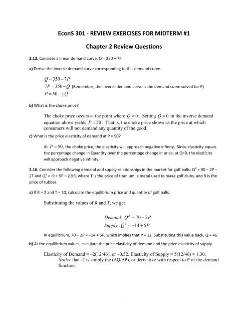
EconS 301 ‐ REVIEW EXERCISES FOR MIDTERM #1Chapter 2 Review Questions2.12. Consider a linear demand curve, Q = 350 – 7Pa) Derive the inverse demand curve corresponding to this demand curve.Q = 350 − 7P7P= 350 − QP = 50 −17Q(Remember, the inverse demand curve is the demand curve solved for P)b) What is the choke price?The choke price occurs at the point where Q = 0 . Setting Q = 0 in the inverse demandequation above yields P = 50. That is, the choke price shows us the price at whichconsumers will not demand any quantity of the good.c) What is the price elasticity of demand at P = 50?At P = 50, the choke price, the elasticity will approach negative infinity. Since elasticity equalsthe percentage change in Quantity over the percentage change in price, at Q=0, the elasticitywill approach negative infinity.2.16. Consider the following demand and supply relationships in the market for golf balls: Q d = 90 – 2P –2T and Q S = ‐9 + 5P – 2.5R, where T is the price of titanium, a metal used to make golf clubs, and R is theprice of rubber.a) If R = 2 and T = 10, calculate the equilibrium price and quantity of golf balls.Substituting the values of R and T, we getdDemand : Q = 70 − 2PsSupply : Q = −14+ 5PIn equilibrium, 70 – 2P = –14 + 5P, which implies that P = 12. Substituting this value back, Q = 46.b) At the equilibrium values, calculate the price elasticity of demand and the price elasticity of supply.Elasticity of Demand = –2(12/46), or –0.52. Elasticity of Supply = 5(12/46) = 1.30.Notice that -2 is simply the (∆Q/∆P), or derivative with respect to P of the demandfunction.1

c) At the equilibrium values, calculate the cross‐price elasticity of demand for golf balls with respect tothe price of titanium. What does the sign of this elasticity tell you about whether golf balls and titaniumare substitutes or complements?10εgolf , ti tan ium= −2() = −0.43. The negative sign indicates that titanium and golf balls are46complements, i.e., when the price of titanium goes up the demand for golf ballsdecreases. Remember that people like to consumer complements together so the increasein the price of one is essentially like an increase in the price of the other, and therefore,the demand will decrease.2.20. Suppose that the market for air travel between Chicago and Dallas is served by just two airlinesmUnited and American. An economist has studied this market and has estimated that the demand curvesfor round‐trip tickets for each airline are as follows: = 10,000 – 100P U + 99P A (United’s demand) = 10,000 – 100P A + 99P A (American’s demand)Where P U is the price charged by United, and P A is the price charged by American.a) Suppose that both American and United charge a price of $300 each for a round‐trip ticket betweenChicago and Dallas. What is the price elasticity of demand for United flights between Chicago andDallas?QQdUdU= 10000 − 100(300) + 99(300)= 9700dUsing PU= 300 and Q = 9700 givesU⎛ 300 ⎞ε QP ,=− 100⎜⎟=−3.09(Simply plug numbers into the price elasticity of demand⎝9700⎠equation)b) What is the market‐level price elasticity of demand for air travel between Chicago and Dallas whenboth airlines charge a price of $300? (Hint: Because United and American are the only two airlinesserving the Chicago‐Dallas market, what is the equation for the total demand for air travel betweenChicago and Dallas, assuming that the airlines charge the same price?)Market demand is given bywe have…Q = Q + Q . Assuming the airlines charge the same priced d dU A2

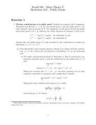
dQ = 10000 − 100P + 99P + 10000 − 100P + 99PdQ = 20000 − 100P+ 99P− 100P+99P(P A and P U simply become P)Qd= 20000 −2PU A A UdWhen P = 300, Q = 19400. This implies an elasticity equal toε QP ,⎛ 300 ⎞=− 2 ⎜ ⎟=−.0309⎝19400⎠Chapter 3 Review Questions3.4. Consider the utility function U(x,y) = y√ with the marginal utilities MU x = y/(2√) and MU y = √.a) Does the consumer believe that more is better for each good?Since U increases whenever x or y increases, more of each good is better. This is also confirmedby noting that MU x and MU y are both positive for any positive values of x and y .b) Do the consumer’s preferences exhibit a diminishing marginal utility of x? Is the marginal utility of ydiminishing?yb) Since MUx= , as x increases (holding y constant), MU2 xxfalls. Thereforethe marginal utility of x is diminishing. However, MUy= x . As y increases, MU y doesnot change. Therefore the preferences exhibit a constant, not diminishing, marginalutility of y.3.13. Draw indifference curves to represent the following types of consumer preferences.a) I like both peanut butter and jelly, and always get the same additional satisfaction from an ounce ofpeanut butter as I do from 2 ounces of jelly.In the following pictures, U 2 > U 1 .3

Jelly42U 11 2U 2Peanut Butterb) I like peanut butter, but neither like nor dislike jelly.JellyU 1 U 2Peanut Butterc) I like peanut butter, but dislike jelly.JellyU 1U 2Peanut Butterd) I like peanut butter and jelly, but I only want 2 ounces of peanut butter for every ounce of jelly.4

JellyU 1U 22124Peanut Butter3.15. Consider the utility function U(x,y) = 3x + y, with MU x = 3 amd MU y = 1.a) Is the assumption that more is better satisfied for both goods?2. Yes, the “more is better” assumption is satisfied for both goods since bothmarginal utilities are always positive. As you add more of either x or y, the total utilityincreases.b) Does the marginal utility of x diminish, remain constant, or increase as the consumer buys more of x?Explain.The marginal utility of x remains constant at 3 for all values of x. The MU x equation is simply aconstant of 3, so the change in x or y doesn’t change MU x .c) What is MRS x,y ?b) MRS 3 (because MU x /MU y =3/1=3)x, y=d) Is the MRS diminishing, constant, or increasing as the consumer substitutes x for y along anindifference curve?TheMRS ,remains constant moving along the indifference curve (look at above equation).x ye) On a graph with x on the horizontal axis and y on the vertical axis, draw a typical indifference curve (itneed not be exactly to scale, but it needs to reflect accurately whether there is a diminishing MRS x,y ).Also indicate on your graph whether the indifference curve will intersect either or both axis. Label thecurve U 1 .5

YU 1U 2Xf) On the same graph draw a second indifference curve U 2 , with U 2 >U 1 .(See above graph)3.21. Suppose a consumer’s preferences for two goods can be represented by the Cobb‐Douglas utilityfunction U = Ax α y β , where A, α, and β are positive constants. The marginal utilities are MU x = αAx α – 1 y βand MU y = βAx α y β – 1 . Answer all parts of Problem 3.15 for this utility function.a) Yes, the “more is better” assumption is satisfied for both goods since both marginal utilities arealways positive.b) Since we do not know the value of α , only that it is positive, we need to specify threepossible cases:When α < 1, the marginal utility of x diminishes as x increases.When α = 1, the marginal utility of x remains constant as x increases.When α > 1, the marginal utility of x increases as x increases.c)MRS x , yα −1αAxyα ββAxyβ=−1=αyβ xd) As the consumer substitutes x for y , the MRSx , ywill diminish because x is in the denominator anddrives down the entire fraction.e & f) The graph below depicts indifference curves for the case where A = 1 and α = β = 0.5.Thus0.5 0.5U ( x,y)= x y . Regardless, the indifference curves will never intersect either axis.6

Y450400350300250200150100500U 2U 10 5 10 15 20 25 30 35X3.24. One type of Cobb‐Douglas utility function is given by U(x,y) = x α y 1‐α , where MU x = αx α‐1 y 1‐α and MU y= (1‐α)x α y ‐α . Suppose that you are told that a person with Cobb‐Douglas preferences has an MRS x,y of 4when x = 4 and y = 8. What is the numerical value of α?First, the expression for MRS x,y isc)MRSx,yMU=MU==αxxyα −( 1−α)α y1−αx1 1−yαx yα−α(plugging in the MU’s and then rearranging)Since we know that MRS x,y = 4 when x = 4 and y = 8,d)α 84 =1−α4α2 =1−α(we set MRS equal to 4 and then plug in x,y values and solve for2 − 2α= αα =23α)7

Chapter 4 Review Questions4.2. The utility function that Ann receives by consuming food F and clothing C is given by U(F,C) = FC + F.The marginal utilities of food and clothing are MU F = C + 1 and MU C = F. Food costs $1 a unit, andclothing costs $2 a unit. Ann’s income is $22.a) Ann is currently spending all of her income. She is buying 8 units of food. How many units of clothingis she consuming?3. If Ann is spending all of her income then…F + 2C= 228 + 2C= 22(Simply plugging in what we know to the Budget Line)2C= 14C = 7b) Graph her budget line. Place the number of units of clothing on the vertical axis and the number ofunits of food on the horizontal axis. Plot her current consumption basket.Remember: Use the Budget Line and set P y to zero to find horizontal intercept and P x equal tozero to find the vertical intercept.1210Clothing864200 5 10 15 20 25 30 35Foodc) Draw the indifference curve associated with a utility level of 36 and the indifference curve associatedwith a utility of 72. Are the indifference curves bowed in toward the origin?Yes, the indifference curves are convex, i.e., bowed in toward the origin. Also, note thatthey intersect the F-axis.8

80Clothing706050403020100U=72U=360 5 10 15 20 25 30 35Foodd) Using a graph (and no algebra), find the utility‐maximizing choice of food and clothing. That is, findthe intersection of the budget line and the indifference curves.80Clothing706050403020100U=72U=36Optimum at F=12, C=50 5 10 15 20 25 30 35Foode) Using algebra, find the utility maximizing choice of food and clothing.The tangency condition requires thatMUFP =F (where slope of BL equals slope of IC)MUCPCPlugging in the known information yields9

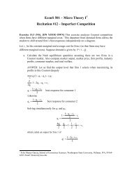
C + 1 1=F 22C+ 2 = FSubstituting this result into the budget line, F + 2 C = 22 results in(2C+ 2) + 2C= 224C= 20C = 5Finally, plugging this result back into the tangency condition implies that F = 2 (5) + 2 = 12 . At theoptimum the consumer chooses 5 units of clothing and 12 units of food.f) What is the marginal rate of substitution of food for clothing when utility is maximized? Show thisgraphically and algebraically.C + 1 5 + 1 1MRS F , C= = = The marginal rate of substitution is equal to the price ratio.F 12 2g) Does Ann have a diminishing marginal rate of substitution of food for clothing? Show this graphicallyand algebraically.Yes, the indifference curves do exhibit diminishing MRSFC ,. We can see this in thegraph in part c) because the indifference curves are bowed in toward the origin.Algebraically, MRS =C+1. As F increases and C decreases along an isoquant,MRS diminishes.FC ,FC ,F4.3. Consider a consumer with the utility function U(x,y) = min(3x,5y), that is, the two goods are perfectcomplements in the ratio 3:5. The prices of the two goods are P x = $5 and P y = $10, and the consumer’sincome is $220. Determine the optimum consumption basket.This question cannot be solved using the usual tangency condition. However, you can seefrom the graph below that the optimum basket will necessarily lie on the “elbow” ofsome indifference curve, such as (5, 3), (10, 6) etc. If the consumer were at some otherpoint, he could always move to such a point, keeping utility constant and decreasing hisexpenditure. The equation of all these “elbow” points is 3x = 5y, or y = 0.6x. Thereforethe optimum point must be such that 3x = 5y.The usual budget constraint must hold of course. That is, 5 x + 10y= 220 . Combiningthese two conditions, that is, plugging y into the budget line, we get (x, y) = (20, 12).10

y(10,6)(20,12)(5,3)4.7. Helen’s preferences over CDs (C) and sandwiches (S) are given by U(S,C) = SC + 10(S + C), with MU C =S + 10 and MU S = C + 10. If the price of a CD is $9 and the price of a sandwich is $3, and Helen can spenda combined total of $30 each day on these goods, find Helen’s optimal consumption basket.See the graph below. The fact that Helen’s indifference curves touch the axes shouldimmediately make you want to check for a corner point solution.To see the corner point optimum algebraically, notice if there was an interior solution, thetangency condition implies (S + 10)/(C +10) = 3, or S = 3C + 20. Combining this with thebudget constraint, 9C + 3S = 30, we find that the optimal number of CDs would be givenby 18C = −30which implies a negative number of CDs. Since it’s impossible topurchase a negative amount of something, our assumption that there was an interiorsolution must be false. Instead, the optimum will consist of C = 0 and Helen spending allher income on sandwiches: S = 10.Graphically, the corner optimum is reflected in the fact that the slope of the budget line issteeper than that of the indifference curve, even when C = 0. Specifically, note that at(C, S) = (0, 10) we have P C / P S = 3 > MRS C,S = 2. Thus, even at the corner point, themarginal utility per dollar spent on CDs is lower than on sandwiches. However, sinceshe is already at a corner point with C = 0, she cannot give up any more CDs. Thereforethe best Helen can do is to spend all her income on sandwiches: (C, S) = (0, 10). [Note:At the other corner with S = 0 and C = 3.3, P C / P S = 3 > MRS C,S = 0.75. Thus, Helenwould prefer to buy more sandwiches and less CDs, which is of course entirely feasible atthis corner point. Thus the S = 0 corner cannot be an optimum.]x11

4.15. Paul consumes only two goods, pizza (P) and hamburgers (H) and considers them to be perfectsubstitutes, as shown by his utility function: U(P,H) = P + 4H. The price of pizza is $3 and the price ofhamburgers is $6, and Paul’s monthly income is $300. Knowing that he likes pizza, Paul’s grandmothergives him a birthday gift certificate of $60 redeemable only at Pizza Hut. Though Paul is happy to get thisgift, his grandmother did not realize that she could have made him exactly as happy by spending far lessthan she did. How much would she have needed to give him in cash to make him just as well off as withthe gift certificate?Paul’s initial budget constraint is the line AC, allowing him to purchase at most 50 hamburgersor at most 100 pizzas. The $60 cash certificate shifts out his budget constraint without changingthe maximum number of hamburgers that he can buy. The new budget constraint is ABD and hecan now buy a maximum of 120 pizzas.Hamburgers605550ABC D20 100 120PizzaInitially, Paul’s optimal basket contains all hamburgers and no pizza, at point A where (P,H) = (0, 50), because MU H /P H = 4/6 > MU P / P P = 1/3. His utility level at point A is U(0,50) = 200. When he gets the gift certificate, Paul’s optimal basket is at point B, spending12

all of his regular income on hamburgers and the $60 gift certificate on pizza. So point Bis where (P, H) = (20, 50) with a utility of U(20, 50) = 220.However, Paul could also achieve a utility of 220 by consuming 220/4 = 55 hamburgers.To buy the extra 5 hamburgers he would require 5*6 = $30. So, if he had received a cashgift of $30 it would have made Paul exactly as well off as the $60 gift certificate forpizzas.4.22. Darrel has a monthly income of $60. He spends this money making telephone calls home(measured in minutes of calls) and no other goods. He mobile phone company offers him two plans:• Plan A: pay no monthly fee and make calls for $0.50 per minute.• Plan B: Pay a $20 monthly fee and make calls for $0.20 per minute.Graph Darrell’s budget constraint under each of the two plans. If Plan A is better for him, what is the setof baskets he may purchase if his behavior is consistent with utility maximization? What baskets mighthe purchase if Plan B is better for him?Let x denote the number of phone calls, and y denote spending on other goods. Under Plan A,Darrell’s budget line is JLM. Under Plan B, it is JKLN. These budget lines intersect at point L, orabout x = 67.y6040JKLMN67 120 200 xIf we know that Darrell chooses Plan A, his optimal bundle must lie on the line segmentJL. No point between L and M would be optimal under this plan because then Darrellcould have chosen a point under Plan B, between L and N, that would have given himmore minutes, and left him with more money to buy other goods. However, we cannotexclude point L itself (Darrell could, for instance, have perfect complements preferenceswith an “elbow” at point L). Thus, if Darrell chooses Plan A his optimal basket could beanywhere between J and L, including either of these points.Similarly, if he chose Plan B then his optimal basket must lie between L and N. Anypoint between L and K (but not including point L) would be dominated by a point under13

Plan A between L and J. Thus, if Darrell chooses Plan B his optimal basket could beanywhere between L and N, including either of these points.Chapter 5 Review Questions5.7 David has a quasi‐linear utility function of the form U(x, y) = x + y , with associated marginalutility functions MU x= 1 and MU y=1.2 xa) Derive David’s demand curve for x as a function of the prices, P x and P y . Verify that the demand for xis independent of the level of income at an interior optimum.Denoting the level of income by I, the budget constraint implies that1 ptangency condition is2 x = pdepend on the level of income.xy, which means thatpx x + p y y = I and the2p yx = . The demand for x does not24 p xb) Derive David’s demand curve for y. Is y a normal good? What happens to the demand for y as P xincreases?From the budget constraint, the demand curve for y is,I − ppx x I yy = = − .p p 4 pYou can see that the demand for y increases with an increase in the level of income,indicating that y is a normal good. Moreover, when the price of x goes up, thedemand for y increases as well.yyx5.19 Lou’s preferences over pizza (x) and other goods (y) are given by U(x,y)=xy, with associatedmarginal utilities MU x =y and MU y =x. His income is $120.a) Calculate his optimal basket when P x =4 and P y =1.yUsing the tangency condition, = 4 , and the budget constraint, 4 x + y = 120 ,xy = 4x Insert int o budget constraint4x + 4 x =1204(15) + y =1208x =120y = 60x =15Lou’s initial optimum is the basket (x, y) = (15, 60) with a utility of 900.14

) Calculate his income and substitution effects of a decrease in the price of food to $3.yFirst we need the decomposition basket. This would satisfy the new tangency condition, = 3xwould give him as much utility as before, i.e. xy = 900 .andy = 3xx(3x) = 900x 2 = 300x =17.3217.32y = 900y = 51.9This gives ( x , y)= (10 3,30 3)or approximately (17.3,51.9). Now we need the final basket, whichsatisfies the same tangency condition as the decomposition basket and also the new budget constraint:3 x + y = 120.yx = 3y = 3x3x + 3x =1206x =120x = 203(20) + y =120y = 60Together, these conditions imply that (x, y) = (20, 60). The substitution effect is therefore 17.3 – 15 =2.3, and the income effect is 20 – 17.3 = 2.7.c) Calculate the compensating variation of the price change.The compensating variation is the amount of income Lou would be willing to give up after the pricechange to maintain the level of utility he had before the price change. This equals the differencebetween the consumer’s actual income, $120, and the income needed to buy the decomposition basketat the new prices. This latter income equals: 3*17.3 + 1*51.9 = 103.8. The compensating variation thusequals 120 – 103.8 = $16.2.d) Calculate the equivalent variation of the price change.The equivalent variation is the amount of income that Lou would need to be given before the pricechange in order to leave him as well off as he would be after the price change. After the price change hisutility level is 20(60)=1200. Therefore the additional income should be such that it allows Lou toypurchase a bundle (x, y) satisfying the initial tangency condition, = 4 , and also such that xy = 1200.xThis implies that ( x , y)= (10 3,40 3)or approximately (17.3, 69.2). How much income would Louneed to purchase this bundle under the original prices? He would need 4(17.3) + 69.2 = 138.4. That is he15

would need to increase his income by (138.4 – 120) dollars in order to be as well off as if the price ofpizza were to decrease instead. Therefore his equivalent variation is $18.4.5.20 Carina buys two goods, food F and clothing C, with the Utility function U=FC+F. Her marginalutility of food is MU f = C+1 and her marginal utility of clothing is MU c =F. She has an income of $20. Theprice of clothing is $4.a) Derive the equation representing Carina’s demand for food, and draw this demand curve for prices offood between 1 and 6.MU F = C + 1 MU C = FTangency: MU F /MU C = P F / P C . (C + 1)/ F = P F /4 => 4C + 4 = P F F. (Eq 1)Budget Line: P F F + P C C = I . P F F + 4C = 20. (Eq 2)Substituting (Eq 1) into (Eq 2): 4C + 4 + 4C = 20. Thus C = 2, independent of P F .From the budget line, we see that P F F + 4(2) = 20, so the demand for F is F = 12/P F65P F4321Demand for food2346F12b) Calculate the income and substitution effects on Carina’s consumption of food when the price risesfrom 1 to 4, and draw a graph illustrating these effects. Your graph does not need to be to scale, but itshould be consistent with the data.Initial Basket: From the demand for food in (a), F = 12/1 = 12, and C = 2.Also, the initial level of utility is U = FC + F = 12(2) + 12 = 36.Final Basket: From the demand for food in (a), we know that F = 12/4 = 3, and C = 2. (Also, U = 3(2) + 3 =9.)Decomposition Basket: Must be on initial indifference curve, with U = FC + F = 36 (Eq 5)Tangency condition satisfied with final price: MU F /MU C = P F / P C . (C + 1)/ F = 4/4 => C + 1 = F. (Eq 3)Eq 5 can be written as F(C + 1) = 36. Using Eq 3, (C + 1) 2 = 36, and thus, C = 5. Also, by Eq 3, F = 6.So the decomposition basket is F = 6, C = 5.Income effect on F: F final basket – F decomposition basket = 3 – 6 = ‐3.Substitution effect on F: F decomposition basket – F initial basket = 6 – 12 = ‐6.16

c) Determine the numerical size of the compensating variation (in monetary terms) associated with theincrease in the price of the good from 1 to 4.P F F + P C C = 4(6) + 4(5) = 44. So she would need an additional income of 24 (plus her actual income of 20).The compensating variation associated with the increase in the price of food is‐24.Clothing 111098Initial U765Final UDecomp Basket4Final BL3Initial Basket21FinalDecomp BLInitial BL001234567891011121314151617181920IncEffectSubst Effect = -6Food5.22 There are two consumers on the market: Jim and Donna. Jim’s utility function is U(x,y)=xy, withassociated marginal utilities MU x =y and MU y =x. Donna’s utility function is U(x,y)=x 2 y, with associatedmarginal utility functions MU x =2xy and MU y =x 2 . Income of Jim of I J =100 and income of Donna is I D =150.a) Find optimal baskets of Jim and Donna when the price of y is P y =1 and price of p is x.Jim’s optimal basket is a solution to equationsMU x / MU y = P / P y and P x + P y y = I J .Hence, we have 2xy / x 2 = P and P x + y = 100with solution x = 200 / (3P) and y = 100 / 3.Analogous system of equations for Donna isy / x = P and P x + y = 150 with solution x = 75 / P and y = 75.b) On separate graphs plot Jim’s and Donna’s demand schedule for x for all values of P.Approximate shape of the demand curve for Jim and Donna is depicted below.17

P xxc) Compute and plot aggregate demand when Jim and Donna are the only consumers.Aggregate Demand:D x (P) = 200 / (3P) + 75 / P = 445 / (3P).d) Plot aggregate demand when there is one more consumer that has identical utility function andincome as Donna.When there is one more consumer that has preferences identical to Donna’s then her demand isalso 75 / P and hence aggregate demand isD x (P) = 200 / (3P) + 75 / P + 75 / P = 650 / (3P).Shape of the demand curve in this case is the same as in part b).18

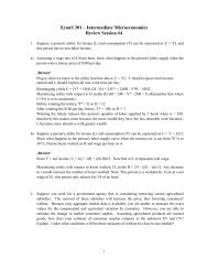
5.28 Consider Noah’s preference for leisure (L) and other goods (Y), U(L,Y) = L + Y . Theassociated marginal utilities are MU L= 1 and MU Y= 12 L2 Y . Suppose that P Y=$1. Is Noah’ssupply of labor backward bending?If Noah’s wage rate is w, then the income he earns from working is (24 – L)w. Since P Y = 1, the number ofunits of other goods he purchases is Y = (24 – L)w. Also, the tangency condition gives us2Combining the two conditions, w L = (24 − L)w , orY = w . L24L = . Clearly, the amount of leisure thatw + 1Noah consumes decreases with an increase in the wage rate, and this is true no matter what the wagerate is. Since the amount of labor that Noah supplies equals (24 – L), we see that his supply of laboralways increases with an increase in the wage rate. So, his labor supply curve is always positively sloped– that is, it is not backward bending.Chapter 6 Review Questions6.4 Suppose that the production function for DVDs is given by Q=KL 2 ‐L 3 , where Q is the number ofdisks produced per year, K is machine‐hours of capital, and L is man hours of labor.a) Suppose K=600. Find the total product function and graph it over the range L=0 and L=500. Thensketch the graphs of the average and marginal product functions. At what level of labor L does theaverage product curve appear to reach its maximum? At what level does the marginal product curveappear to reach its maximum?Total Product with K=600Total Product35,000,00030,000,00025,000,00020,000,00015,000,00010,000,0005,000,000-0 100 200 300 400 500 600 700Labor19

AP and MP with K=600200000AP/MP1000000-100000-200000-300000-400000AP0 100 200 300 400 500 600 700MPLaborBased on the figure above it appears that the average product reaches its maximum at L = 300. Themarginal product curve appears to reach its maximum at L = 200b) Replicate the analysis in (a) for the case in which K=1200Total Product with K=1200Total Product300,000,000250,000,000200,000,000150,000,000100,000,00050,000,000-0 500 1000 1500Labor20

AP and MP with K=12001000000500000AP/MP0-500000-1000000-1500000-20000000 200 400 600 800 1000 1200 1400APMPLaborBased on the figure above it appears that the average product curve reaches its maximum at L =600. The marginal product curve appears to reach its maximum at L = 400.c) When either K=600 or K=1200, does the total product function have a region of increasing marginalreturns?In both instances, for low values of L the total product curve increases at an increasing rate. For K =600, this happens for L < 200. For K = 1200, it happens for L < 400.6.9 Suppose the production function is given by the equation Q = L K . Graph the isoquantscorresponding to Q=10, Q=20, Q=50. Do these isoquants exhibit diminishing marginal rate of technicalsubstitution?Capital7.06.05.04.03.02.01.00.0Q=10 Q=20Q=500 20 40 60 80Labor21

Because these isoquants are convex to the origin they do exhibit diminishing marginal rate oftechnical substitution.6.11 Suppose the production function is given by the following equation (where a and b are positiveconstants): Q=aL+bK. What is the marginal rate of technical substitution of labor for capital (MRTS L,K ) atany point along an isoquant?For this production functionMPL= a and MPKMRTSLK ,= b. The MRTSLK ,is thereforeMPL= =MPKab6.12 You might think that when a production function has a diminishing marginal rate of technicalsubstitution of labor for capital, it cannot have increasing marginal products of capital and labor. Showthat this is not true, using the production function Q=K 2 L 2 , with the corresponding marginal productsMP K =2KL 2 and MP L =2K 2 L.First, note that MRTS L,K = L/K, which diminishes as L increases and K falls as we movealong an isoquant. So MRTS L,K is diminishing. However, the marginal product of capitalMP K is increasing (not diminishing) as K increases (remember, the amount of labor isheld fixed when we measure MP K .) Similarly, the marginal product of labor is increasingas L grows (again, because the amount of capital is held fixed when we measure MP L ).This exercise demonstrates that it is possible to have a diminishing marginal rate oftechnical substitution even though both of the marginal products are increasing.6.17 What can you say about returns to scale of the linear production function Q=aK+bL, where a andb are positive constants.Q = aK + bL= λaK + λbL= λ[aK + bL= λ[Q]Therefore a linear production function has constant returns to scale.6.18 What can you say about the returns to scale of the Leontief production function Q=min(aK,bL),where a and b are positive constants?A general fixed proportions production function is of the form Q = min( aK,bL).22

Q = min(aK,bL)= min(λaK,λbL)= λmin(aK,bL)= λ[Q]Therefore the production function has constant returns to scale.6.19 A firm produces a quantity Q of breakfast cereal using labor L and material M with theproduction function Q = 50 ML + M + L . The marginal product functions for this production functionareMP L= 25 M L +1MP M= 25 L .M +1a) Are the returns to scale increasing, constant, or decreasing for this production function?To determine the nature of returns to scale, increase all inputs by some factor λand determine if output goes up by a factor more than, less than, or the same as λQ = 50 λMλL + λM + λLλQλ= 50λ ML + λM + λLQλ= λ ⎡50ML M L⎤⎣+ +⎦Q = λQλBy increasing the inputs by a factor of λ output goes up by a factor of λ . Since output goes up bythe same factor as the inputs, this production function exhibits constant returns to scale.b) Is the marginal product of labor ever diminishing for this production function? If so, when? Is it evernegative, and if so, when?The marginal product of labor isMMPL= 25 + 1LSuppose M > 0 . Holding M fixed, increasing L will have the effect of decreasing MPL. Themarginal product of labor is decreasing for all levels of L . The MPL, however, will never benegative since both components of the equation above will always be greater than or equal tozero. In fact, for this production function, MPL≥ 1.23

6.25 A firm’s production function is initially Q = KL , with⎛ L ⎞⎛ K ⎞MP K= 0.5⎜⎟ and MP L= 0.5⎜⎟ . Over time, the production function changes to⎝ K ⎠⎝ L ⎠⎛Q = K L, with MP K= L and MP L= 0.5 K ⎞⎜ ⎟ .⎝ L ⎠a) Verify that this change represents technological progress.With any positive amounts of K and L, KL < K L so more Q can be produced with the finalproduction function. So there is indeed technological progress.b) Is this change labor saving, capital saving, or neutral?With the initial production functionWith the final production functionMRTSLK ,MPL0.5K= =MP LK.For any ratio of capital to labor, MRTS L,K is lower with the second production function.Thus, the technological progress is labor-saving.24