School of Economic Sciences - Washington State University

1 IntroductionDuring the week of October 16, 2005, Tennessee Governor Phillip Bredesen (D) headed an officialtrip to Japan.In addition to the governor, the delegation included other public officials andmore than 50 representatives of private firms.The stated goal of the mission was to “...[use]this experience to create new opportunities for Tennessee businesses and workers as we make ourpresentation to the international community” (Bredesen to Conduct Asian Trade Mission 2005). 1This is not the first time a Tennessee governor traveled to Japan with the claim of state exportpromotion. During the ten year interval from 1997–2006, Gov. Bredesen and his predecessor Gov.Don Sundquist (R) undertook five trade missions to Japan (in 1998, 1999, 2000, 2003, and 2005).During that time, Japan was Tennessee’s third largest export destination, behind Canada andMexico.Trade missions such as Tennessee’s are a potential form of public investment to increase exportsand enhance development. Unlike public investment, a large literature exists on private investment.Roberts and Tybout (1997) find evidence of significant fixed costs for firms to enter a foreign market.Rauch (1999) and Andersson (2007) find these fixed costs are market specific, and depend on thefamiliarity of the source country with the destination. Melitz (2003) uses these fixed costs in atheory of private investment where monopolistic competitors, differing in productivity, choose topay the fixed cost and export, or not. Arkolakis (2008) constructs a model where firms must investin advertisements to build market awareness of their products. Firms choose how much to advertiseand whether or not to export to each country.For many firms, the entry fixed cost is enough to prohibit exporting. Bernard and Jensen (1995)report only 10% of U.S. firms export to any destination. Eaton, Kortum, and Kramarz (2004) find,of the firms that do exports, many export to only a few countries.Thus there may be a rolefor government, interested in promoting exports, to reduce a market specific fixed cost to export,and increase the access of domestic firms to consumers they otherwise are unable to reach. Thismay be done directly by the government subsidizing individual firms or industries. Trade missions,however, are potentially able to decrease the entry cost for all firms in the state by increasing the1 http://www.tennesseeanytime.org/governor/viewArticleContent.do?id=645 (accessed Nov. 6 2007).1

familiarity of the target country.Governor-led trade missions are one piece of the state export promotion repertoire. Other toolsinclude trade offices, translators and professionals specializing in a specific region, and missionsled by other officials such as commerce chairs. Unlike some of these other export promotion expenditures,governor-led trade missions are easily observable and cleanly measurable. I create adata set of every governor-led trade mission from each U.S. state by searching through local mediareports during the ten year period from 1997–2006. Further, I know the target country of eachtrade mission. There is a high level of activity: more than five hundred such missions. Nearlytwenty states go on at least one trade mission per year. Furthermore, as the example of Tennesseeand Japan shows, many missions are repeat trips.Besides the trade mission data, I obtain data on state exports to each country in the world.This is the only state export data with destination information available. Together with the trademission data, I know both how much each state exports to each country and how much publicinvestment there is in the target country in terms of governor-led trade missions.I develop a model of the cross-sectional relationship between state exports and state trademissions, tying theory to the data. The model is an extension of the Melitz (2003) model of tradeas modified by Chaney (2008). The Melitz model features monopolistic competitors, differing byproductivity, that export by paying both a variable cost and a market specific entry cost. Because ofthis export fixed cost, only highly productive firms export. Chaney’s extension allows for asymmetryacross many countries.I introduce a new agent, the state government, to Chaney’s model. The state government is theonly agent with access to a costly technology, trade missions, that decreases the effective fixed costof exporting to the visited country for all firms in that state. I define and solve for an equilibriumwhere government chooses the optimal frequency of trade missions to each country. The modelaccounts for unobserved heterogeneity for individual states and individual countries. This controlsfor the possibility the governor of Tennessee may want to visit Japan because Japan is a largeeconomy or because Japan is an interesting place to visit. The model predicts a strong relationshipbetween trade missions and state exports for state-country pairs that have a relatively large exportrelationship. The economics is similar to that of a sales representative visiting existing customers2

to increase sales further.From the derived structural equation relating trade missions to state exports, I estimate theexport elasticity of missions using the trade mission and export data I collected. I compare theestimated export elasticity from the data to a null hypothesis where trade missions are trips torandom destinations. Rejecting this random hypothesis is a necessary, but not sufficient, conditionfor trade missions to have a positive impact on exports.As both the trade mission and state export data have source and destination information, I amable to control for individual state and individual country characteristics. I find there is a significantrelationship between state exports and state missions. Governors travel to destinations with whomthey have a large export relationship relative to other destinations. Thus I reject the random model.This finding holds up under several different regression specifications and estimators.Previous literature on export promotion as potential public investment focuses on estimatingthe impact of a trade mission on exports using differences in panel data. Wilkinson, Keillor, andd’Amico (2005) find a positive impact on state expenditures promoting exports whereas Bernardand Jensen (2004) do not.Neither of these papers have destination information for exports orexport promotion. They compare the difference in total state expenditure on export promotionagainst the difference in total state exports. Besides the limitation of not knowing which countriesare targeted for export promotion, they do not have a particularly clean measure of state promotionexpenditures.Nitsch (2007) and Head and Ries (forthcoming) study the impact of national trade missions onnational exports. They both use national export and trade mission data with destination information.They estimate the impact of trade missions led by country leaders on exports by differencingsource-target pairs across time using panel data. Again there are conflicting results. 2 Cassey (2007)estimates the impact of a governor-led trade mission on state exports. Initial estimates indicatea significant increase in state exports from a state trade mission.However, accounting for thepotential simultaneity bias in exports and missions, he is unable to reject the hypothesis that state2 Rose (2007) uses the location of embassies and national trade data to find if the presence of an embassy increasesnational exports. He finds an embassy increases exports by 6%–10%. Kehoe and Ruhl (2004) suggest the largerelative increase in Wisconsin exports to Mexico after NAFTA compared to Minnesota is due to the presence of aWisconsin trade office in Mexico.3

trade missions do not have an impact on state exports to the visited country on average.The conflicting results from the literature are due to features of the panel data they use. First,on the state level, the large amount of noise in the export data may overwhelm a reasonablysized effect in state exports from a trade mission; the imprecision of the estimates may hide asignificant impact. Second, the timing of the treatment is difficult to pin down because missionsoccur frequently, as in the case of Tennessee and Japan. The lag time for its effects is unknown.Most importantly, the literature does not have an explicit theory for how missions affect exports.The potential endogeneity of missions and exports does not allow for a suitable exogenous treatment.Thus estimation of the average impact of a trade mission on exports to the visited country usingpanel data differences has not yielded a convincing estimate.2 A Model of State Exports with Trade Missions2.1 The Melitz-Chaney Model of International TradeConsider the model described in Chaney (2008). This model features asymmetric countries differingin market specific entry costs. Chaney expands the model introduced by Melitz (2003) in whichmonopolistic competitors, differing in productivity, decide whether to export or not. 3 The model iscross-sectional and there is neither aggregate nor individual uncertainty.There are J countries differing in endowments of the only resource, labor. The endowment isdenoted as N j for each country j. Labor is immobile across countries.Consumers in all countries have identical preferences and may be aggregated into a singlerepresentative with a taste for variety:( ∫) σU j = x j (0) 1−µ × x j (ω) σ−1 σ−1 µσ dω (1)Ω jwhere x indicates the quantity consumed, ω is the particular variety, Ω j is the set of availablevarieties in country j, µ ∈ (0, 1) is the income share spent on the set of varieties, and σ > 1 isthe elasticity of substitution between varieties. Varieties are assumed to be imperfect substitutes3 Helpman, Melitz, and Rubinstein (2008) describe a similar model.4

for one another. Labor does not reduce utility. The representative consumer in different countriesfaces a different set of available goods, Ω j .Good 0 is produced by a constant returns to scale production function where one unit oflabor makes w j units of good 0, q j (0) = w j (0)l j (0). This good is traded competitively and freelythroughout the world.Besides production of good 0, in each country there are monopolistic competitors, each producingone particular variety ω. The measure of monopolistic competitors active in each countryis L j . This measure of active firms is exogenously given, but is proportional to the aggregate laborendowment N j . No two potential competitors anywhere in the world produce the same good ω.Therefore knowing the variety ω pins down the country of production of ω.Labor is perfectlymobile across varieties and good 0 within each country.Monopolistic competitors differ in the goods they produce as well as their productivity, φ.Across and within countries, active firms know their permanent productivity φ(ω), which is therealization of a random variable Φ drawn from a Pareto distribution with support [1, ∞) andparameter γ:Pr(Φ ≤ u) = H(u) = 1 − u −γ . (2)Let γ > 0. The parameter γ indicates the heterogeneity of productivity: larger γ indicatesfirms are more similar since the mass of firms is more tightly packed. The Pareto distribution is astandard modeling choice because of its analytic simplicity.Production by firm ω for sale in country j depends on the productivity of firm ω and the laborit uses to sell to j: q j (φ(ω)) = φ(ω)l j (φ(ω)).Any of the varieties may be traded. There is a variable cost to trade given by τ ij . If τ ij unitsof a variety are shipped from i to j then one unit arrives (Samuelson 1954). Assume τ jj = 1 forall j, τ ij > 1 for all i ≠ j, and the triangle inequality holds. The transportation cost need not besymmetric so it is possible τ ij ≠ τ ji . There is also a fixed cost for firms in i who export to j givenby f ij > 0 for i ≠ j and f jj = 0. Similar to τ ij , assume the triangle inequality holds for f ij andsymmetry need not hold. The fixed cost is paid in units of labor by the exporting firm. Thesetrade costs are identical for all firms in the same country; they do not depend on the productivity5

of firms.The cost of delivering q units from i to j by a firm with productivity φ:⎧⎪⎨c ij (φ) =⎪⎩w i τ ijφ q ij(φ) + w i f ij : q ij (φ) > 00 : q ij (φ) = 0(3)and profits:π ij (φ) = p ij (φ)q ij (φ) − c ij (φ).Because costs, production, and profits depend on productivity and not the particular good, onemay switch between describing goods with ω, φ(ω), or φ as convenience dictates.Therefore,q j (ω) = q j (φ(ω)) = q ij (φ), l j (ω) = l j (φ(ω)) = l ij (φ), p j (ω) = p j (φ(ω)) = p ij (φ), andπ j (ω) = π j (φ(ω)) = π ij (φ). There is no need for a source subscript when the variety ω is knownbecause each variety is uniquely produced in the world.As in Chaney (2008), I only consider equilibria in which every country produces good 0 and themeasure of monopolistic competitors is proportionally fixed based on the labor force of the country.Good 0 is set to be the world wide numeraire. Its price is fixed to one in every country. Givenp(0) = 1 in every country, the labor productivity of producing good 0 in country j, w j , is the wagein country j, justifying (3).Because there is no free entry, monopolistic competitors may receive positive profits. The profitsfrom all firms in country j, Π j are redistributed to the consumer in country j. Thus the aggregateincome of country j is Y j = w j N j + Π j . The only substantive difference with this model and theChaney model is each country retains its own profits.I require each country to retain its ownprofits so state government has something to maximize with trade missions.An equilibrium is the set of available goods in each country, {Ω ∗ j }J j=1 and the associated productivitythresholds for operating there, { ˆφ ∗ ij }J i=1 ; consumption in each country for all goods availablethere, {x ∗ j (0)}J j=1 and {x∗ j (ω)|ω ∈Ω∗ j }J j=1 ; prices for each variety in each country that are producedat a positive level, {p ∗ j (0)}J j=1 and {p∗ j (ω)|ω ∈ Ω∗ j }J j=1 ; the wage in each country, {w∗ j }J j=1 ; aggregateprofits in each country {Π ∗ j }J j=1 ; and the production plans for each firm selling a positive amount ineach country, { ( qj ∗(0), l∗ j (0)) } J j=1 and {( qj ∗(ω), l∗ j (ω)) |ω ∈ Ω ∗ j }J j=1 ; such that the following conditions6

hold.• Good 0: q ∗ j (0) > 0, p∗ (0)w j (0) = w ∗ j , and q∗ j (0) = w j(0)l ∗ j (0), ∀j and ∑ Jj=1 q∗ j (0) = ∑ Jj=1 x∗ j (0).• Given prices, labor endowment, wages, profits, and the set of available goods, the representativeconsumer in each country maximizes (1) by choosing x ∗ (0) and x ∗ (ω) such thatp ∗ j (0)x j(0) + ∫ Ωp ∗ ∗ j (ω)x j(ω)dω ≤ wj ∗N j + Π ∗ j and x j(0), x j (ω) ≥ 0 ∀ω ∈ Ω ∗ j .j• Given wages, transportation and fixed costs, and the demand function for its good in eachcountry, each monopolistic competitor chooses p ∗ j (ω) to maximize ∑ Jj=1 p j(ω)q ∗ j (ω) − c∗ j (ω).• Individual goods and labor clearing condition: qj ∗(ω) = x∗ j (ω) and q∗ j (ω) = φ(ω)l∗ j (ω), ∀j∀ω.• Country labor clearing condition: ∑ Jk=1(l∗k(0) + ∫ L jk(l ∗ k (ω) + f jk) dω ) = N j , ∀j where L jk isthe measure of country j firms exporting to k.• Country profits condition: ∫ L j( ∑ Jk=1 π∗ k (ω)) dω = Π ∗ j , ∀j.• Ω ∗ j determined by L j and { ˆφ ∗ ij }J i=1 where ˆφ ∗ ij = sup {πij ∗ (φ) = 0}.φ≥1With a continuum of varieties, the equilibrium is identical under either Bertrand competitionor Cournot competition. Chaney (2008) proves the existence of this equilibrium for γ > σ − 1 > 0.Henceforth, all variables are assumed to be at their equilibrium values and thus the stars aredropped. Equilibrium properties include the following.Firms from i selling in country j set the price p j(φ(ω))= pij (φ) =σσ−1w i τ ijφ. For some firms,their productivity is low enough that there does not exist a price such that π ij (φ) ≥ 0. Thereforefor each (i, j) there exists a threshold productivity, ˆφ ij such that firms in i with φ < ˆφ ij choose notto export to j. Among other fundamentals and parameters, this threshold productivity dependson the fixed cost to export f ij :( σˆφ ij =µγγ − (σ − 1)) 1γ× Y− 1 γj( )wi τ ij× (w i f ij ) 1σ−1 . (4)θ jAs f ij increases, the threshold productivity is larger. Notice because f ii = 0, all L i firmsproduce domestically. Using (2), the measure of firms in i exporting to j is L ij = L i(1 − H( ˆφij ) ) .7

In (4), θ j is the multilateral resistance term representing country j’s remoteness from the restof the world. The multilateral resistance term is defined in variable costs, fixed costs, and goodsavailability:where a =θ j =J∑i=1L − 1 γiw i τ ij × (w i f ij ) a γγσ−1− 1 > 0. The multilateral resistance term takes into account how the firm heterogeneityparameter γ and the variable and fixed cost terms affect the measure of firms selling incountry j, and thus the aggregate price level facing consumers in country j.Interating the exports from those firms whose productivity is greater thanˆ φ ijobtains theequilibrium aggregate exports from i to j. This involves solving for q j (ω(φ)) = q ij (φ) using thefundamentals of L i , w i , f ij , τ ij , and H(φ):∫ ∞˜X ij = L i p ij (φ)q ij (φ)dH(φ)ˆφ ij= µL i Y j(θjw i τ ij) γ× (w i f ij ) −a . (5)Aggregate exports from i to j increase in the measure of firms in i, the income in j, and thedifficulty in j of receiving exports from all other countries, θ j . Aggregate exports decrease in thetransportation and fixed costs to export.2.2 Adding GovernmentDeparting from the Melitz-Chaney model, I introduce a new agent in each country called government,or alternatively the governor. The government is the sole agent with access to a technologythat, for a cost, decreases the effective fixed cost to export for all firms located in that country.This technology is the trade missions the governor of i takes to j.The effective fixed cost facing all potential exporters in i to j is η ij and depends on the untreatedfixed cost to export, f ij , and the trade mission intensity, m ij . For modeling purposes, m ij is a realnumber indicating trade mission durations and quality otherwise missing from the model.Theeffective fixed cost:η ij (m ij ) =z b f ij(z + m ij ) b .8

If there are zero trade missions then η ij = f ij . The reduction in the effective fixed cost diminishesin trade mission intensity and has an elasticity of −bm ij /(z + m ij ). Let M ij = z + m ij . Thereforeb is the elasticity with respect to M ij . The z parameter is a curvature parameter that may bethought of as the common mission intensity that has already occurred.The cost associated with trade missions depends on the source i and the target j. The governmentin i has total trade mission expenditure ofJ∑G i = d i g j (M ij − z).j=1The interpretation of d i is the opportunity cost of the governor’s time. The opportunity cost oftime does not depend on the visited country. The g j represents the cost of organizing each instantof a mission to j, which is common to all governments visiting j. There is no cost from travelingon zero missions. 4The government pays for the trade mission expenditure, G i , with a proportional labor tax t i .Before proceeding, let me reinterpret the Melitz-Chaney model for U.S. states. Consider U.S.states as a subset of the countries in the model. Henceforth they are indexed by i as the source forboth exports and missions. Destinations are countries, not other states. The country index is j.The equilibrium with government is similar to the Melitz-Chaney equilibrium in section 2.1.The representative’s budget changes to (1 − t i )w i N i + Π i for states, but remains Y j = w j N j + Π jfor countries. The government in each state maximizes the income of the representative consumerby choosing a labor tax rate and trade mission intensity to all countries in the world.Assumption 1. The measure of potential exporters in state i, L i , is exogenously fixed proportionalto state size N i .Assumption 1 simplifies the analysis by preventing a general equilibrium effect of trade missionson firm entry. In the Melitz (2003) model, the measure of domestic producers is endogenously determinedas the result of a continuum of potential firms paying a fixed cost to learn their productivity4 Again, trade missions are investment in a costly technology for decreasing the fixed cost to all potential exporters.It is neither the case that trade missions pay the difference between f ij and η ij, or a fraction thereof, for each actualexporter, nor is it the case the target country receives income from expenditures on f ij, η ij, or M ij.9

and then deciding to domestically produce or not. Subsequently, domestic firms choose whether toexport or not. With free entry, the expected firm profits, net of the cost to learn their productivity,is zero.Conditional on producing domestically, firm profits are nonnegative with some strictlypositive. Melitz shows the measure of actual firms is proportional to domestic country size, N j ,thus justifying the assumption of a fixed measure of firms in section 2.1. With the introductionof government, the expected profits before knowing one’s productivity are a function of trade missions.Thus more firms may choose to enter domestically than without government since they knowgovernment will lower the effective export fixed cost to some countries. Assumption 1 prevents this.Assumption 2. The multilateral resistance term θ j does not depend on mission intensity.Assumption 2 keeps the definition of θ j using f ij rather than replacing it with η ij . The implicationis missions from state i do not open up country j to potential exporters from another statek. Together assumptions 1 and 2 appear strong. However they are approximately true in the limitas the benefit and cost of a trade mission go to zero. See appendix A for details.The following lemma shows the equilibrium relationship between trade missions and state exports.Lemma 1. Equilibrium aggregate exports from i to j as a function of trade missions,( ) γ (θj1abX ij (M ij ) = µL i Y j (w i f ij ) −a × ij)w i τ ij z M= ˜X ij ×( 1z M ij) ab,where a =γσ−1 − 1 > 0 and b, z > 0, is increasing in M ij.This proof, as well as all others, is in appendix A.Trade missions increase aggregate state i exports to j. The increase in state exports is dueentirely to exports from firms whose productivity is not great enough to cover f ij , but is greatenough to pay η ij . The exports from firms willing to pay f ij do not change if instead thesefirms actually pay η ij , though their profit increases. Therefore trade missions increase total stateexports entirely through the extensive margin. Furthermore, M ij does not impact X ik ; there is no10

diversionary impact of missions. Lemma 1 also says missions are more effective if firms are morehomegenous (γ is large), but less effective if goods are more substitutable (σ is large).Trade missions increase state exports. Lemma 2 says they increase state profit also.Lemma 2. State profit as a function of trade missions,Π s (M i,1 , M i,2 , ..., M i,J ) = σ − 1σγis increasing in M ij .J∑j=1= σ − 1σγ z−ab( ) γ (θj1abµL i Y j (w i f ij ) −a × ij)w i τ ij z MJ∑j=1˜X ij × M abij ,Trade missions increase state profits through their effect on exports, though the increase inprofits is less than the increase in exports. The government faces a tradeoff: trade missions andincreased state profit versus the expense of higher labor taxes reducing state disposable income.Given the strategies of consumers, firms, and other governments, a governor chooses t ∗ i and {M ij ∗ }J j=1to solvemax(1 − t i )w i N i + Π i (M i1 , ..., M iJ ) such that t i w i N i ≥ G i and t i ≥ 0, M ij ≥ z. (6)Theorem. An equilibrium exists in which trade mission intensity from i to j is given by{ γ − (σ − 1)M ij = maxγ{ γ − (σ − 1)= maxγ(µ θjL i Y jσd i g j}1Xij ˜ , zσd i g j) γ }(w i f ij ) −a , zw i τ ijIn order for an equilibrium to exist, parameters must satisfy 0

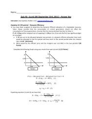
The theorem says optimal mission intensity inversely depends on the state and country-specificmission costs, d i and g j , and the default difficulty in penetrating the foreign country, f ij .Optimalmission intensity is increasing in the size of the foreign country, and the size of the state.These fundamentals are summarized by ˜X ij , the state exports in the absence of government action.Therefore the model predicts a positive relationship between untreated exports and missions.This result is not obvious.One may have thought trade missions would be most effectiveif the target country was not a large export destination without government. Then governmentinvestment would open the country up for exports. On the contrary, optimal mission intensity isgreater for targets where there is a large export relationship in the absence of government. Theeconomics underlying this result are displayed in figure 1.Figure 1 displays the pdf for the Pareto distribution (2). Consider the case of a target countrywith large threshold productivity, ˆφ1 . It does not matter if this high threshold is due to smallcountry size, which affects all states equally, or high transportation costs or high f, which affectsthe match between a state-country pair.Since ˆφ 1 is large, there is a small mass of firms withproductivity greater than ˆφ 1 . A trade mission reduces the effective fixed cost and the thresholdproductivity to ˆφ 2 . The additional aggregate exports accrue exclusively from the extensive margin:the exports of new exporters induced by the lower effective fixed cost. The extensive margin isthe mass of firms between ˆφ 1 and ˆφ 2 . There is no change in exports from those with productivitygreater than ˆφ 1 because in this model, the general equilibrium effects of θ are suppressed, and thusa decrease in the fixed cost does not affect exports for a firm with productivity above ˆφ 1 .Now consider the impact of a mission to another country identical to the first except for a lowerthreshold productivity, ˆφ3 . There is a much larger export relationship with this second countrywithout government because there is a larger mass of firms to the right of ˆφ3 than ˆφ 1 . A missionto this country reduces the fixed cost and the threshold productivity to ˆφ 4 . Again the additionalstate exports are from the extensive margin, the mass of firms between ˆφ 3 and ˆφ 4 . It is clear fromfigure 1 there is a far greater mass of new exports from a mission to the second country comparedto the first. This effect is greater the larger is γ because this puts more mass in the left tail atthe expense of the right tail. Though firms with productivity between ˆφ 1 and ˆφ 2 each export morethan any firm with productivity between ˆφ 3 and ˆφ 4 , the difference in aggregate is more than made12

Figure 1. Economics of the theorem. The graph is the pdf for the Pareto distribution with γ = 3. The additionalmass of new exporters from a mission decreasing the threshold productivity from ˆφ 1 to ˆφ 2 is less than the additionalmass of new exporters from a mission decreasing the threshold productivity from ˆφ 3 to ˆφ 4.up for by the mass of new exporters. Thus optimal missions target countries with a large exportrelationship without government.2.3 A Reduced Form EquationThe theorem relates trade missions to ˜X ij , the aggregate exports in the absence of government.However there can be no data on ˜X ij because most states do in fact travel on trade missions.Therefore ˜X ij needs to be replaced with actual exports X ij using lemma 1:X ij = ˜X ij ×( 1z M ij) ab. (7)To make this switch, revisit the government’s problem, (6). By lemma 2, the government’s problembecomesσ − 1maxM i,1 ,...,M i,J σγ z−abJ∑j=1˜X ij M abij − d iJ∑g j (M ij − z) .j=1Taking derivatives, taking logs, using the substitution (7), and solving yieldslog M ij = log σ − 1σγ ab + log X ij − log d i − log g j . (8)13

It is feasible to take the log of ˜X ij because each country has a continuum of varieties and there isno real valued upper support on the productivity distribution. There is always a mass of exporting(firms L ij = L i 1 − H( ˆφij ) ) > 0 regardless of the size of ˆφ ij .Equation (8) shows the relationship between bilateral state exports and bilateral state trademissions controlling for state and country characteristics, d i and g j . The reduced form equation (8)predicts the export elasticity of trade missions is one relative to each state-country pair. Howeverthis is with respect to M ij .The variation in the model comes from the bilateral trade costs τ ij and f ij . Since state andcountry characteristics are accounted for by d i and g j , the variation in X ij is driven by the qualityof state-country matches in τ ij and f ij . For reasons outside of the model, some state-country pairshave a good match, and thus there is a large export relationship and a strong motive for sendingtrade missions. Other state-country pairs are not a good match. The quality of the match may bethought of as the relative geography or the relative immigrant history of state-country pairs.3 A Description of the DataEquation (8) relates actual state exports to actual state trade missions (plus z) controlling for stateand country characteristics. To see if the estimate for the export elasticity of missions is positiveas it is in (8) requires state level data on trade missions and exports by destination. I compilethe trade missions data by searching through local media sources from all states for 1997–2006.Appendix B contains the details of the trade mission collecting process. State export data comesfrom a data set compiled by the U.S. Bureau of the Census that is rarely used in the internationaltrade literature. It is the Origin of Movement (OM) state export data available for purchase fromthe World Institute of Strategic Economic Research. Cassey (2009) provides the details for thecollection of the OM data.The OM data are the only state export data with the destinationinformation available.14

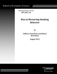
Figure 2. Country RGDP and state trade missions. Mean is the average of real GDP from 1997–2006. Point labelsare the 3-letter ISO country code. Axes are log base 2 scale. Countries receiving zero missions are not included.3.1 The State Trade Mission DataDuring the ten years from 1997 through 2006, there are 512 governor-led U.S. state trade missions.This is roughly fifty-five trade missions per year. The most missions occurred in 1997 (81) followedby 1999 (70). The fewest missions occurred in 2001 (29). Each year around 20 states travel on atleast one trade mission. I only consider trade missions to countries with 1997 GDP data availablefrom the IMF. This reduces the number of missions to 503.Out of 176 destinations with GDP data, 117 (66.48%) of these never host a trade missionduring the ten year period. The average 1997 GDP of destinations that never host a trade missionis $12.52 billion whereas it is $713 billion for those that do host a trade mission. Thus there is astrong relationship between the size of a country and the number of missions it hosts. Figure 2shows this relationship, where the size of a country is given by the mean of its real GDP over the1997–2006 period.The largest destinations not visited are Turkey ($186 billion GDP in 1997), Saudi Arabia ($165billion), and Iran ($106 billion). The smallest destinations visited are Tonga ($0.18 billion), Laos($1.76 billion), Senegal ($4.41 billion), and Ghana ($6.88 billion). There are 37 destinations to host15

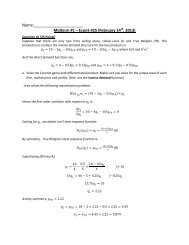
a trade mission with GDP smaller than Turkey’s.Japan is the most frequent destination for governor-led trade missions. It is visited 67 timesfrom 1997–2006.Other frequent destinations are China (45), Mexico (39), Germany (37), andTaiwan (31). Though Japan is the most frequent destination, China holds the record for most tripsin a single year: 11 in 2005. Japan is next with ten in 2005. The most frequent state-country tripis Virginia to Germany which occurs five times over the ten years. Also, Tennessee to Japan andOregon to Japan occurs five times.Visited countries tend to be larger than non-visited countries, however visited countries growless quickly. The correlation between 1997 GDP of the destination and the total number of tripsthere between 1997 and 2006 is 0.82. Compare this to 0.46 which is the correlation of 1997 GDPwith total exports to the country, or 0.44 which is the correlation between 1997 GDP and the totalnumber of states exporting to the country pooled across panels. The correlation between the totalnumber of trips and the average GDP growth rate is -0.10. This is similar to the correlation of thenumber of exporting states with the average GDP growth rate.Virginia took the most trips, visiting foreign destinations 31 times in ten years. Other stateswith a large number of trips are Wisconsin (30), Nebraska (23), and Ohio (21). The governorsof Connecticut, Nevada, South Dakota, and Wyoming did not travel to any country on a trademission. The average state has 10.08 trade missions from 1997–2006. The most missions per yearis by Wisconsin. In 1997 the governor of Wisconsin, Tommy Thompson, went on 12 trade missions.The average number of trips per year is 2.4 for states with at least one trade mission during 1997to 2006.States with the most missions tend to be slightly larger in terms of their total value of manufacturingshipments (TVS), although, as seen in figure 3, the relationship between size and thenumber of missions is not strong. The correlation between the total number of trade missions takenby states during 1997–2006 and their 1997 TVS is 0.22. It is -0.26 between trips and TVS growth.The correlation between TVS and missions is much less than the correlation of TVS with eitherstate exports (0.89) or the number of states exporting (0.78).Figures 2 and 3 provide a nice overview of the state trade mission data and of which countrieshost missions and which states travel frequently. They are incapable of showing any relationship16

Figure 3. State total value of manufacturing shipments and state trade missions. Mean is the average of real TVSfrom 1997–2006. Axes are log base 2 scale. Connecticut, Nevada, South Dakota, and Wyoming are not includedsince they do not have any missions from 1997–2006.between exports and missions as predicted by the theorem. Thus I introduce data on state exportsby destination.3.2 The State Export DataU.S. state export data (OM) to 242 foreign destinations are available, though not well known toacademic audiences. I use export data from all 50 U.S. states to the 176 countries with 1997 IMFGDP data, in correspondence with the trade mission data. The data are measured at the port ofexit by compiling forms required of those exporting more than $2500 in a shipment. Cassey (2009)provides complete details of the OM data, including its collection.The OM data are the only state export data with destination information. Because the dataare collected before any shipments leave the U.S., the quality of the data does not depend on thedestination country.Another attractive feature of the OM data is, unlike other Census data sets, there is no Censussuppression to protect individual exporter’s identities. There is, however, a low-value threshold of17

$2500. That is, there must be at least one shipment from state i to country j of at least $2500to be included in the data. On a state scale, this low-value threshold is easily satisfied. However,nearly 20% of state-country observations are zero. Given no Census edits and the small low-valuethreshold, these zeros reflect “true” zeros.I only use state export data from odd-numbered years during 1997–2006. Exports are deflatedusing the annualized Producer Price Index for All industrial commodities less fuel. 5Since the export data are collected at the port of exit rather than in the state of production,it is possible the OM data do not reflect state exports for two reasons. First, the OM data includeinland freight costs which may overestimate exports from interior states. Second, the OM datamay underestimate exports from interior states because exports consolidated at a port state areattributed to the port state. Ignoring the destination information, Cassey (2009) compares the OMdata to a destination-less state export data set based on the Annual Survey of Manufactures. Hefinds on average the OM data measure state exports for manufacturing exports relatively accurately,albeit noisily. There is evidence of consolidation, however, for Florida and Texas. For this reason,I only use manufacturing state export data in the sections that follow. Agricultural and miningexports are removed from consideration because the OM state exports are not reliable for state oforigin of production.Combining the state trade mission and state export data yields one observation where thereis a trade mission to a country with whom the traveling state does not export: in 2000 Vermontvisited Laos. Laos is the only country included that does not have normal trade relations with theUnited States for much of the study period. Though arranged in 1997, Congress did not approvenormal trade relations with Laos until 2004.4 Comparing Model Predictions to Regression EstimatesThe theory in section 2 yields a prediction of the export elasticity of missions as given in (8). Themodel’s elasticity is one. I use the data described in section 3 to estimate the same elasticity in the5 Source: U.S. Bureau of Labor Statistics, http://data.bls.gov/cgi-bin/surveymost?wp. Accessed June 11, 2007.18

data. The regression equation corresponding to (8):log M ij = β 0 + β 1 log X ij + δ i + ζ j + ε ij , (9)where δ i is the coefficient on a state dummy and ζ j is the coefficient on a country dummy. Iassume ε ij includes measurement error. The state and country dummies attempt to deal with anyunobserved heterogeneity. Heteroskedasticty is present in the data.The null hypothesis of trade mission travel to random countries is rejected if estimates for β 1are significantly different from zero. The data must reject the random hypothesis in order for trademissions to have any hope as effective public investment in export promotion. A rejection of thenull hypothesis indicates trade missions are traveling to countries that make economic sense basedon the model. It does not mean there is a statistically significant impact of state trade missions onstate exports.Notice the image in figure 2 can be reproduced by the model.But figure 2 could also beproduced with an alternative model in which governor’s choose to visit destinations by throwingdarts at a weighted map of the world. If these visits are just about politics, then governors wouldtend to visit locations with large economies (which will also be where the states tend to have largeexports). Therefore it is crucial to difference out the unobservable individual characteristics thatwould attract a politically motivated governor to get at the underlying match between states andcountries.4.1 Estimation and ResultsThe model and corresponding regression equation may be thought of as in the long run and requiringcross-sectional estimation. However the data are longitudinal. To transform the panel data intoa cross section, I treat every year as exactly the same. Thus I sum the number of missions fromstate i to country j over the ten year period from 1997 – 2006. I average real state manufacturingexports from i to j in odd-numbered years over the same period to use for actual exports, X ij .The averaging over years eliminates most zeros in the export data. There are 176 × 50 = 8800observations for trade mission intensity and state exports.Of these, 719 (8.2%) state-country19

pairs are never export partners during 1997–2006. Thus log-linearizing as in (9) loses nonrandomobservations. This potentially introduces selection bias in estimates using the ordinary least squaresestimator (OLS), though the the fact that only 8% are zero suggests this bias will be small if itexists.The sets of state and country binary variables in (9) control for unobserved heterogeneity inindividual state and individual country characteristics. Because the model and regression equationare a long run cross-section, the data is not differenced over time for each state-country pair. Ideal with issues of causality and simultaneity bias using the state and country binary variables.Minimizing the simultaneity bias is crucial because finding an instrument is difficult as one maysuspect from the scattered points in figure 3.Since M ij = z + m ij , equation (9) is a nonlinear equation with numerous dummies. I estimatethis in a two step procedure. First I estimate z holding the other coefficients fixed at one. ThenI plug in the estimated value of z and use the OLS estimator to find an estimate of β 1 and thecoefficient for each dummy variables.Table 1 shows the OLS estimates for β 1 . The first column is the estimate for β 1 when all 50states and 176 countries are included. I weight observations by the mean RGDP of the destinationcountry. This weight diminishes the noise from the many small countries making up a tiny portionof U.S. manufacturing exports. The standard errors are state-country adjusted. Notice the estimateon β 1 is significantly different from zero.Because of the potential for bias by dropping only those observations with zero exports, I repeatthe estimation by restricting the number of countries to the 50, 10, and 5 largest in terms of meanRGDP. All 50 states export to the top 10 countries. 6 The top 10 countries account for 63% of U.S.manufacturing exports.In all cases, the estimated elasticity, β 1 , is significantly different from zero. Given the state andcountry dummies, the significance of β 1 indicates governors travel to countries for which they havea relatively large export relationship compared to all other potential export partners. Because thesets of binary variables control for size, it is not the case that big states travel or big countries are6 The top countries ranked by mean RGDP are Japan, Germany, United Kingdom, France, China, Italy, Canada,Spain, Brazil, and Mexico.20

Table 1.OLS Estimates of Export Elasticity of Missions using 50 Stateslog(z + m ij ) = β 0 + β 1 log X ij + δ i + δ j + ε ij10 countries 20 countries 50 countries 176 countriesz 0.0243 ∗∗ 0.041 ∗∗∗ 0.144 ∗∗∗ *0.144* ∗∗(0.477) (0.255) (0.201) –β 1 0.411 ∗∗∗ 0.275 ∗∗∗ 0.102 ∗∗∗ 0.075 ∗∗∗(0.1346) (0.0788) (0.0237) (0.0147)N 500 1000 2484 8081ˆR 2 0.439 0.427 0.428 0.430Notes: Observations are mean RGDP weighted. Standard errors are robust to state-countrypairs. State and country dummy coefficients are estimated but not reported.∗∗∗∗ indicate significance at the 99% level.targeted. Also, the binary variables control for behavior such as the opening up of a destination toall states uniformly.Since β 1 > 0, I reject the random destinations hypothesis. However, the estimates are significantlydifferent from one also. There are several reasons why the estimates may not be one even iftrade missions are motivated by increasing state income.First, a drawback of restricting data to manufactures is trade missions from primarily agrarianstates presumably increase agricultural exports not manufacturing exports. Therefore in additionto the regressions with all 50 states, I estimate (9) without the 16 states with an agriculture andmining share of GDP above 10%. 7 Table 2 shows these estimates. The β 1 estimates increasesomewhat, but so do the standard errors.Similarly, I estimate β 1 without Florida and Texas, the two states Cassey (2009) finds evidence ofmanufacturing export consolidation. Removing Florida and Texas does not increase the estimates.Another reason the OLS estimates on β 1 may not be one is, in the model, M ij takes real values.In the data, M ij is a count. Though I have data on the duration of each mission in days for 85% oftrade missions, the trip duration includes travel time which depends on the location of the targetcountry. Thus using days instead of the count of missions may bias estimates since mission to Asiancountries are necessarily longer.7 The states in order of most agriculture and mining as a share of GDP are Alaska, Wyoming, North Dakota, NewMexico, Louisiana, Nevada, Texas, Oklahoma, West Virginia, South Dakota, Hawaii, Nebraska, Idaho, Colorado, andKansas.21

Table 2.OLS Estimates of Export Elasticity of Missions using top 34 Manufacturing Stateslog(z + m ij ) = β 0 + β 1 log X ij + δ i + δ j + ε ij10 countries 20 countries 50 countries 176 countriesz 0.077 ∗∗ 0.331 ∗∗∗ 0.366 ∗∗∗ *0.366*(0.251) (0.230) (0.192) –β 1 0.403 ∗∗ 0.164 ∗∗ 0.094 ∗∗ 0.070 ∗(0.166) (0.0683) (0.044) (0.0361)N 250 1000 2484 8081ˆR 2 0.425 0.424 0.422 0.425Notes: Observations are mean RGDP weighted. Standard errors are robust to state-country pairs. Stateand country dummy coefficients are estimated but not reported.∗∗∗ , ∗∗ , ∗ indicate significance at the 99%, 95%, and 90% levels respectively.Table 3.PPML Estimates of Elasticity of Exports on Missions using all 50 statesz + m ij = exp(β 0 + β 1 log X ij + δ i + δ j ) ˆε ij10 countries 20 countries 50 countries 176 countriesz 0.0243 ∗∗ 0.041 ∗∗∗ 0.144 ∗∗∗ *0.144* ∗∗(0.477) (0.255) (0.201) –β 1 .281 ∗∗∗ 0.265 ∗∗∗ 0.193 ∗∗∗ 0.182 ∗∗∗(.0996) (0.0802) (0.0557) (0.0523)N 500 1000 2484 8081Notes: Observations are mean RGDP weighted. Standard errors are state-countryadjusted. State and country dummy coefficients are estimates but not reported.∗ , ∗∗ indicate significance at the 99% and 95% levels respectively.Count data, such as the cumulative number of missions, commonly follows a Poisson distribution.Because of this, I estimate β 1 using a Poisson pseudo-maximum liklihood estimator (PPML).Besides handling the count data of the trade missions, Santos Silva and Tenreyro (2006) point outthe PPML handles the extreme heteroskedasticity common in international trade data biasing OLSestimates on log-linearized data (as well as affect the standard errors). Table 3 contains the resultsfrom the PPML.Similar to table 1, the PPML estimates of β 1 are significantly different from zero. The fact theestimate for β 1 obtained through the data is significant with the binary variables indicates thereis some bilateral relationship between exports and missions beyond individual state and individualcountry characteristics. There is evidence states travel on trade missions to those countries withwhom they have a relatively large export relationship. I reject the random hypothesis.22

5 ConclusionU.S. state governors frequently travel abroad on trade missions. The motive for these trade missions,however, is debatable. Proponents argue they increase state exports to the visited country and stateincome, and thus are a form of public investment in development. Detractors argue trade missionsare a vacation for the governor at taxpayer expense. The panel data approach of resolving thisdebate by testing for a significant change in state exports before and after a governor-led trademission yields conflicting results. In contrast I take a cross sectional approach testing for a weakerbut necessary condition: whether governors travel to random destinations or whether they travelto destinations consistent with a model where trade missions matter for state exports.I find evidence that trade missions are to destinations for which the state is exporting a relativelylarge amount compared to that state’s other export relationships. My data allow me to controlfor the unobserved heterogeneity in individual state and country characteristics.estimate is of the export elasticity of missions relative to the state-country pair.Therefore myI reject therandom destination hypothesis.The model’s predicted elasticity is part of the solution of a reduced form equation derived byadding a benevolent government to the heterogeneous firm monopolistic competition trade modelof Melitz (2003) and Chaney (2008). I solve this extended model for the equilibrium frequencyof trade missions to each country. I derive a relationship between trade missions and actual stateexports. I create a new data set on governor-led trade missions from 1997–2006 containing thedestination information and combine it with a little used data set of state exports, also with thedestination information. Since I know the source state and target countries for both trade missionsand exports, I control for individual state and individual country characteristics in a regression ofthe data.This paper takes a step toward resolving the debate on whether public investment in targetedexport promotion and customer acquisition leads to increased exports and development. It addsto the literature by focusing on one particular targeted export promotion policy—governor-ledtrade missions—that unlike previous work in which investment is private and inferred, is a measurableform of investment. I develop a theory of public investment commensurate with this public23

investment data.ReferencesAndersson, Martin 2007. “Entry Costs and Adjustments on the Extensive Margin” CESIS Electronicworking paper no. 81. http://www.infra.kth.se/cesis/documents/WP%2081.pdf (accessedJuly 2007).Arkolakis, Costas 2008. “Market Penetration Costs and the New Consumers Margin in InternationalTrade” NBER working paper no. 14214.Bernard, Andrew B., and J. Bradford Jensen 1995. “Exporters, Jobs, and Wages in U.S. Manufacturing:1976–1987” Brookings Papers on Economic Activity: Microeconomics 1995, 67–112.2004. “Why Some Firms Export” Review of Economics and Statistics 86 (2), 561–569.Cassey, Andrew J. 2007. “Estimates on the Impact of a State Trade Mission on State Exports”Manuscript, University of Minnesota, 2007.2009. “State Export Data: Origin of Movement vs. Origin of Production” Journal of Economicand Social Measurement 34 (4), 241–268.Chaney, Thomas 2008. “Distorted Gravity: The Intensive and Extensive Margins of InternationalTrade” American Economic Review 84 (4), 1707–1721.Eaton, Jonathan, Samuel Kortum, and Francis Kramarz 2004. “Dissecting Trade: Firms, Industries,and Export Destinations” American Economic Review: Papers and Proceedings 94 (2), 150–154.2010. “An Anatomy of International Trade: Evidence from French Firms” unpublished.Head, Keith, and John Ries forthcoming. “Do Trade Missions Increase Trade?” Canadian Journalof Economics.Helpman, Elhanan, Marc Melitz, and Yona Rubinstein 2008. “Estimating Trade Flows: TradingPartners and Trading Volumes” Quarterly Journal of Economics 123 (2), 441–487.24

International Monetary Fund 2006. World Economic Outlook Database. Washington,DC.http://www.imf.org/external/pubs/ft/weo/2006/01/data/index.htm (accessed December15, 2006).Kehoe, Timothy J., and Kim J. Ruhl 2004. “The North American Free Trade Agreement AfterTen Years: Its Impact on Minnesota and a Comparison with Wisconsin” Center for Urban andRegional Affairs Reporter 34 (4), 1–10.Melitz, Marc J. 2003. “The Impact of Trade on Intra-Industry Reallocations and Aggregate IndustryProductivity” Econometrica 71 (6), 1695–1725.Nitsch, Volker 2007. “State Visits and International Trade” The World Economy 30 (12), 1797–1816.Rauch, James 1999. “Networks Versus Markets in International Trade” Journal of InternationalEconomics 48 (1), 7–35.Roberts, Mark J., and James R. Tybout 1997. “The Decision to Export in Colombia: An EmpricalModel of Entry with Sunk Costs” American Economic Review 87 (4), 545–564.Rose, Andrew K. 2007. “The Foreign Service and Foreign Trade: Embassies as Export Promotion”The World Economy 30 (1), 22–38.Samuelson, Paul A. 1954. “The Transfer Problem and Transport Costs, II: Analysis of Effects ofTrade Impediments” Economic Journal 64 (254), 264–289.Santos Silva, João Manuel Caravana, and Silvana Tenreyro 2006. “The Log of Gravity” Review ofEconomics and Statistics 88 (4), 641–658.Wilkinson, Timothy J., Bruce D. Keillor, and Michael d’Amico 2005. “The Relationship BetweenExport Promotion Spending and State Exports in the U.S.” Journal of Global Marketing 18(3), 95–114.25

AppendicesAProofsAssumptions L i (M ij ) = L i Y j (M ij ) = Y j θ j (M ij ) = θ j .Justification. Suppose governor i may take at most one trade mission to country j. Furthersuppose the parameters and fundamentals, Y j , w i , and τ ij , are such that this governor chooses togo on the mission. I show this decision will not change to zero missions when both the benefit andthe cost of the mission go to zero,limb→0˜X ij M b ij − ˜X ij = 0 and limdi →0 d ig j (M ij − 1) = 0.The notation above matches that in the paper, yet should be viewed generally enough to hold inform when the assumptions do not hold. Let d i and b converge to zero along the same sequence.Compare the rates of convergence. Use l’Hôpital’s rule:limz→0˜X ij M z ij − ˜X ijzg j= limz→0˜Xij M z ij log M ijg j (M ij − 1)= ˜X ij log M ijg j (M ij − 1) > 0.Therefore near the limit, the convergence rate is equal. Since the governor chooses to go on a trademission initially and the rate of convergence is constant in the limit, the governor does not want tochange her mind at any point in the sequence.Lemma 1. Equilibrium aggregate exports from i to j as a function of trade missions,X ij (M ij ) = ˜X ij × M abij ,where a =γσ−1 − 1 > 0 and b > 0, is increasing in M ij.26

Proof. From Chaney, aggregate state i exports to country j are given by (5),( ) γX˜θjij = µL i Y j × (w i f ij ) −a .w i τ ijReplace the untreated fixed cost to export f ij with the effective fixed export cost η ij ,X ij = µL i Y j(θjw i τ ij) γ× (w i η ij ) −awhich is legitimate due to the assumptions. Substitute in for η ij using (2.2), η ij = f ij. PositiveMijbfirst derivative shows state exports are increasing in missions:dX ijdM ij= ab ˜X ij M ab−1ij> 0for a, b > 0 and M ij ≥ 1. Since there is no upper bound on the Pareto distribution, ˜Xij > 0; thereis always a mass of firms with productivity greater than the threshold ˆφ ij .Lemma 2. State profit as a function of trade missions,Π s (M i,1 , M i,2 , ..., M i,J ) = σ − 1σγJ∑j=1˜X ij × M abij ,is increasing in M ij .Proof. By definition,Π i =J∑j=1L i∫ ∞ˆ φijπ ij (φ)dH(φ).σ w i τ ijσ−1 φPlug in for ˆφ ij and π ij = p ij (φ)q ij (φ) − c ij (φ) using the equilibrium values of p ij (φ) =( ) −σ−1 ( )and, conditional on exporting at all, q ij (φ) = σ σ γγ wi τ 1−σ ijµφ σ−1 σ−1γYj. Given thedistribution is Pareto, there is an analytic solution,Π i =J∑j=1γ−(σ−1)σ − 1σγ µL iY j(θjw i τ ij) γ(w i η ij ) −( γσ−1 −1) .θ j27

Substitute in η ij = f ij.MijbTheorem. An equilibrium exists in which trade mission intensity from i to j is given by( ) 1σ − 1 abM ij =˜Xijσγ g i g j1−abprovided f ij or d i and g j are small enough so that M ij ≥ 1 ∀i, j and 0 < ab < 1.Proof. The consumer and firms problems solved in Melitz (2003) and Chaney (2008). I show thegovernment’s problem and solution. Set up the Lagrangian from (6). Then the first order necessarycondition:ab σ − 1σγX˜i jMij ab−1 − d i g j = 0.The second order sufficient condition:ab(ab − 1) σ − 1σγ˜X ij M ab−2ij< 0.In order for this to hold with γ > σ − 1 > 0 it must be that ab − 1 < 0. The problem is greatlysimplified with the assumptions because then˜ X ij is treated as a constant by the government.BTrade Mission Data Collection and SourcesData on trade missions are obtained by the author through a Lexis-Nexis Academic search throughlocal news sources. The search is state-by-state, covering the years 1997–2006. Keywords in thesearch are “governor,” “trade,” and “mission.” For some states, the returns to this search were largeand mainly irrelevant. Thus “governor,” “export,” and “mission” are used for some large states.It is common for each trip to include multiple foreign destinations. Each country is counted asa separate trade mission. Furthermore both Hong Kong and Taiwan are counted as destinationsseparate from China. Also if the same destination is visited twice in the same calendar year thenit is counted as two separate trips. The data do not include any visits of foreign delegates in theUnited States, any governor trips for reasons not explicitly stated as “trade missions,” any tripsin which the governor of the state is not present, or any trips that are organized by the Federal28

Government. Finally there must be a local newspaper reference close to the data of departure forthe trip count. Any reference such as “Unlike the governor of X, the governor of Y traveled toJapan in 1984” is not counted.Additional information is the duration of each trade mission in days. These days include traveltime, thus more remote destinations have longer durations than closer destinations even if the timein each host is the same. Travel time is included because news sources near unanimously reportthe time the governor is away from the state rather than the time in each host. Both the taxpayercost of the trip and the number of delegates is reported infrequently and inconsistently and thusare not used.The reason for using only governor-led trade missions is twofold. The governor is an importantenough figure in local, if not national media, that the press makes a record of the trade mission. Thisallows me to compile a list of all trade missions using a standardized source, LexisNexis academic.Also, trade missions vary in importance. The governor provides a signal of the importance of themission. As one trade mission participant said, “We will be viewed as serious people because ourgovernor is supporting us...” (Doyle Goes to China on Businesses’ Dime, Madison Capital Times,March 22, 2004). This is not necessarily the case with other public officials, such as Lt. Governors,commerce chairs, and others, who sometimes lead missions.Trade missions do not directly cost the taxpayer much. Some of the trade mission observationsinclude data on direct public expenditure on the trade mission. Typically the state pays for thegovernor and a few other officials, but private delegates pay for themselves. It is not rare for agrowth promotion organization to sponsor public officials, thus no taxes are used. Out of 183missions for which the public expense is reported in the media, 38 (20.76%) were fully paid forprivately. The average total public outlay for trips using public money is $47,500. The mostexpensive trip recorded cost is $250,000 (North Carolina to China in 1998), a tiny fraction of anystate’s budget. The most significant cost is the time the governor is not in the state, an aspectI model. It is this opportunity cost that is most important in the trade mission debate. I modelthis explicitly. Though the costs of a trade mission are relatively small, the question of its effect isstill important for guiding state policy and for settling a matter of public debate. If in fact trademissions do increase state exports, then their low cost is one of their most attractive characteristics.29