A New Prediction Model Based on Belief Rule Base for System's ...

SI et al.: NEW PREDICTION MODEL BASED ON BELIEF RULE BASE FOR SYSTEM’S BEHAVIOR PREDICTION 639TABLE IPATTERN OF TRAINING DATASETX is the input nodes and y denotes the predicted output node.Following successful training, the BRB prediction model canpredict future outcomes y t .In the BRB prediction model, the belief rules can be designedas follows:R k : IF x t−1 is A k 1 ∧ x t−2 is A k 2 ···∧x t−p is A k t−pTHEN ŷ t is {(D 1 ,β 1,k ),...,(D N ,β N,k )} with a(2)II. BEHAVIOR PREDICTION MODEL BASEDON BELIEF RULE BASEA. <strong>Model</strong> Structure and RepresentationIn this section, the prediction model is investigated in theBRB framework. It is assumed that a set of observed data is providedin the form of input–output pairs (X(t m ),y(t m )),m=1,...,M, with X(t m ) being an input vector of the actual systemat time t m and y(t m ) being a scalar or vector representingthe corresponding output value or subjective distribution valueof the actual system at time t m . In this paper, the input vectorX(t m ) consists of the antecedent attributes associated withsystem output y(t m ) at time t m .In prediction problem, the inputs used in prediction modelare the past input vector, i.e., lagged observations of the currenttime, while the outputs are the future values. Each set of inputpatterns is composed of any moving fixed-length window withinthe time series of the input data. The general prediction modelcan be represented asŷ(t + k − 1) = f(x t−1 ,x t−2 ,...,x t−p ) (1)where ŷ(t + k − 1) represents the predicted value at time t,(x t−1 ,x t−2 ,...,x t−p ) is a vector of lagged variables, and prepresents the dimensions of the input vector (number of inputnodes) or the number of past inputs related to the futurevalue. Although multistep prediction may capture some systemdynamics, the performance may be poor due to the accumulationof errors. In practice, one-step-ahead prediction results aremore useful since they provide timely information for preventiveand corrective maintenance plans [57]. In addition, in viewsof Wang [52] and Zhang et al. [69], the more the step is ahead,the less reliable the forecasting operation. Thus, this study onlyconsiders one-step-ahead prediction, that is, k =1, in (1). Forsimplicity, let X(t) =(x t−1 ,x t−2 ,...,x t−p ) denotes the inputvector of the prediction model.B. Construction of Belief-Rule-Base Systemfor Behavior <strong>Prediction</strong>In order to construct BRB prediction model, suppose x t−1 ,x t−2 ,...,x t−p are p antecedent attributes associated withsystem-prediction output ŷ t , and the BRB system approach attemptsto identity the appropriate internal representation betweenX(t) and ŷ t .Table I shows how training patterns can be designed in theBRB prediction model. In Table I, p denotes the number oflagged variables (i.e., so-called embedding dimension), whilet − p represents the total number of data samples. Moreover,rule weight θ k and attribute weight δ 1,k ,δ 2,k ,...,δ M k ,kwhere x 1 ,x 2 ,...,x t−p represents the antecedent attributes inthe kth rule. A k i (with i =1,...,p,k =1,...,L) is the referentialvalue of the ith antecedent attribute in the kth rule andA k i ∈ A i . A i = {A i,j ,j =1,...,J i } is a set of referential valuesfor the ith antecedent attribute and J i is the number ofthe referential values. θ k (∈ R + ,k =1,...,L) is the relativeweight of the kth rule, and δ 1,k ,δ 2,k ,...,δ p,k are the relativeweights of the M k antecedent attributes used in the kth rule.β j,k (j =1,...,N,k =1,...,L) is the belief degree assessedto D j , which denotes the jth consequent corresponding to theoutput value at time t. If ∑ Nj=1 β j,k =1,thekth rule is said tobe complete, else it is incomplete. In addition, suppose that p isthe total number of antecedent attributes used in the rule base.A BRB given in (2) represents functional mappings betweenantecedents and consequents possibly with uncertainty. It providesa more informative and realistic scheme than a simpleIF–THEN rule base for knowledge representation. Note thatthe degrees of belief β i.k and the weights could be assignedinitially by experts or by common sense, and then trained orupdated using dedicated learning algorithms [66]. For simplicity,in the following, let us assume that the relative weight ofith antecedent attribute in belief rule k is the same as the relativeweight of this antecedent attribute in belief rule l, wherek =1,...,L,l =1,...,L,k ≠ l. As such, δ i,k can be representedas δ i (i =1,...,p).C. Strategy for Converting Available Data to Belief StructureWhen applying a BRB, the input of an antecedent is transformedinto a belief structure over the referential values of anantecedent. The distribution is then used to calculate the activationweights of the rules in the rule base. The main advantageof doing so is that precise data, random numbers, and subjectivejudgments with uncertainty can be consistently modeled underthe same framework [59], [63], [64], [66]. In addition, the ERalgorithm is the inference engine of BRB system, but the ERalgorithm is suitable for dealing data in the format of a beliefstructure [59], [62], [63]. Due to the fact that the input data X(t)may be a numerical value or a subjective distribution, there isa need to transform these data into the belief structure. In [62],a rule-based scheme to convert other inputs has been developedto deal with the input information involving quantitativedata. In this paper, rule-based transformation technique can beused for data transformation. For more discussions on this issue,see [62] and [64]. As a result, each input can be represented asa distribution on the referential values using a belief structure.By using the rule-based transformation technique [62], theinput vector X(t) =(x t−1 ,x t−2 ,...,x t−p ) can be described as

640 IEEE TRANSACTIONS ON FUZZY SYSTEMS, VOL. 19, NO. 4, AUGUST 2011TABLE IIREFERENTIAL POINTS OF GYROSCOPIC DRIFTa distribution on referential values using a belief structure asfollows:S(x t−i )={(A i,n ,α n,i (x t−i )),n=1,...,J i }, i =1,...,p(3)where A i,n is the nth referential value of the attribute x t−i ,α n,i (x t−i ) is the matching degree, which measures the matchingdegree of the ith input to its nth referential value, and J i isthe number of the referential values used to describe the ithantecedent attribute. From (3), the mass can only be assignedto the single referential point of the assessment framework.Therefore, the focal elements under such case are always thesingle grade in the assessment framework.In (3), α n,i (x t−i ) could be obtained using different waysin hand, depending on the nature of an antecedent attribute anddata available. Generally, there is a scheme to deal with differenttypes of input information, as summarized below [64], [66].1) Quantitative attributes assessed using referential terms:In this case, if the antecedent attribute x t−i can be assessedby defining independent crisp sets, then α n,i (x t−i )can be obtain through rule-based transformation technique[62]. For example, in the Section IV-C, the assessmentframework for the model inputs is A i = {S, M, L} ={A i,1 ,A i,2 ,A i,3 },fori =1and 2. For intuitive illustration,we used the 35th data point in our dataset to showhow we can obtain the belief structure. As for the 35thdata point, the specific inputs are 1.22 ◦ h −1 and 1.26 ◦ h −1 .Taking the first input, i.e., 1.22 ◦ h −1 , for instance, we canconvert 1.22 ◦ h −1 as S(1.22) = {(A 1,1 , 0.45),(A 1,2 , 0.55),(A 1,3 ,0)} through rule-based transformation techniqueand the referential points in Table II. Specifically, we haveα 1,1 (1.22) = (1.4 − 1.22)/(1.4 − 1), and α 2,1 (1.22) =(1.22 − 1)/(1.4 − 1) based on the rule-transformationtechnique and the referential points in Table II. Other datacan be handled in a similar way, and thus, their descriptionis omitted. As a result, each input can be represented as adistribution on the referential values using a belief structure.If the assessment of x t−i involves fuzziness, thenA i,j can be defined as fuzzy sets and α n,i (x t−i ) can becalculated via membership functions [65].2) Quantitative attributes assessed using interval: In thiscase, there are two ways to model input information inBRB framework. First, the interval can be seen as a specialform of the fuzzy linguistic value; therefore, α n,i (x t−i )can be determined in a way similar to the case 1). Thesecond method is that belief structure can be extended toan interval version [53], and then, α n,i (x t−i ) can be generatedthrough rule-based transformation technique, butα n,i (x t−i ) is also in the format of interval in such a case.For details, see [53].3) Qualitative or symbolic attributes assessed using subjectivejudgments. In this case, the belief degree α n,i (x t−i ) isassigned directly by the decision maker using his subjectivejudgments for each referential value or each symbolicterm. For example, if ε n,i (x t−i ) is the belief degree assignedto the symbolic term or the referential term A i,j bythe decision maker, then α n,i (x t−i )=ε n,i (x t−i ).D. Calculating the Output of Belief-Rule-Base<strong>Prediction</strong> <strong>Model</strong>When the antecedent attribute, such as the inputs of the BRB,is available, the ER approach serves as the inference engine ofBRB prediction model, which mainly consists of following twosteps.1) Step 1: Calculation of the Activation Weight of Belief Rule:The activation weight of the kth rule ω k at time t is calculatedby∏θ M k k i=1ω k (t) =(αk j,i (t − i))¯δ i∑ Ll=1 θ ∏ M kl i=1 (αl j,i (t − andi))¯δ iδ i¯δ i =(4)max i=1,...,Mk {δ i }where δ i,k (∈ R + ,i=1,...,M k ) is the relative weight of theith antecedent attribute that is used in the kth rule. Because ω kwill be eventually normalized so that ω k ∈ [0, 1] using (4), θ kand δ i,k can be assigned to any value in R + . Without loss of generality,however, we assume that θ k ∈ [0, 1](for k =1,...,L)and δ i,k ∈ [0, 1](for i =1,...,M k ). αi,j k (for i =1,...,M k ),which is called the individual matching degree, is the degreeof belief to its jth referential value A k i,j in the kth rule.α k = ∏ M ki=1 (αk i,j )¯δ iis called the normalized combined matchingdegree.2) Step 2: Rule Inference Using the Evidential-ReasoningApproach: Using the analytical ER algorithms [51], the finalconclusion O (ŷ(t)) that is generated by aggregating allrules that are activated by the actual input vector X(t) =(x t−1 ,x t−2 ,...,x t−p ) at time instant t can be represented asfollows:O(ŷ(t)) = F (X(t)) = {(D j , ˆβ j (t)),j =1,...,N} (5)where O(ŷ(t)) denotes the predicted output of prediction modelin the format of belief structure, and ˆβ j (t) denotes the predictedbelief degree in D j at time instant t. The aggregated resultO(ŷ(t)) represents the overall assessment of system’s behaviorand provides a complete picture about the system state at time t,from which one can tell which assessment grades the system’sbehavior is assessed to, and what belief degrees are assigned tothe defined assessment grades D n ,n=1,...,N.In(5), ˆβ j (t)can be formulated as follows [51]:ˆβ j (t) = μ(t) × ∏ L(k=1 ωk (t)β j,k (t)+1− ω k (t) ∑ Ni=1 β i,k(t) )1 − μ(t) × [∏ Lk=1 (1 − ω k (t)) ]− μ(t) × ∏ Lk=1(1 − ωk (t) ∑ Ni=1 β i,k(t) )1 − μ(t) × [∏ Lk=1 (1 − ω k (t)) ] (6)

SI et al.: NEW PREDICTION MODEL BASED ON BELIEF RULE BASE FOR SYSTEM’S BEHAVIOR PREDICTION 641⎡ ()N∑ L∏N∑μ(t) = ⎣ ω k (t)β j,k (t)+1− ω k (t) β i,k (t)j=1 k=1k=1i=1(−1L∏N∑− (N − 1) 1 − ω k (t) β i,k (t))](7)where ω k (t) is calculated by (4). Note that ˆβ j (t) is the functionof β i,k , θ k , δ i , and X(t).As shown in (5), we can see that the default output formatof BRB prediction model is belief distribution. However, insome engineering applications, a numerical output value ŷ(t) isrequired and preferred, such as pipeline-leak detection in [58].To achieve this aim, the concept of utility in decision theoryand utility-based transformation technique [62] can be usedto convert the distributed assessment O (ŷ(t)) to a numericaloutput ŷ(t). It is demonstrated that the two are equivalent in thesense that they both represent the same states of the system [62].For detailed implementation, see [58] and [62].From (6) to (7), it can be seen that belief degrees β i,k , attributeweights δ m , and rule weights θ k play a significant role in the finalconclusion O(ŷ(t)). The degree to which the final output canbe affected is determined by the magnitude of the belief degrees,attribute weights, and rule weights. On the other hand, if the parametersof the BRB prediction model, such as θ k ,δ m , and β j,k ,are not given apriorior only known partially or imprecisely,they could be trained using observed input and output information.Therefore, the inference performance of BRB predictionsystems and the proposed model can be improved if the foregoingunknown parameters with some constraints are adjusted byoptimization algorithm. The construction of the constraints ofthe unknown parameters in BRB prediction model is given asfollows [66].1) A belief degree must not be less than 0 or more than 1,i.e.,i=10 ≤ β j,k ≤ 1, j =1,...,N, k =1,...,L. (8)2) If the kth belief rule is complete, its total belief degree inthe consequent will be equal to 1, i.e.,∑ N β j,k =1. (9)j=1Otherwise, the total belief degree is less than 1.3) A rule weight is normalized, so that it is between 0 and 1,i.e.,0 ≤ θ k ≤ 1, k =1,...,L. (10)4) A attribute weight is normalized so that it is between 0and 1, i.e.,0 ≤ δ i ≤ 1, i =1,...,p (11)As such, there is a need to develop a method that can learnparameters of BRB prediction model using observed input andoutput information. This is exactly discussed in the following.III. PARAMETERS OPTIMIZATION FOR BELIEF-RULE-BASEPREDICTION MODELAs discussed in [64] and [66], belief rule in a BRB may initiallybe provided by human experts based on individual experienceand personal judgments and then optimally trained if theobserved input–output data are available. In addition, a changein unknown parameters θ k ,δ m , and β j,k may lead to changesin the performance of the BRB prediction model. Therefore, itis preferred to construct optimization model for training predictionmodel. Inherited from the training process for general BRBsystem developed in [66], one optimization model is developedto train the proposed prediction model.First, we assume that a set of observation pairs (X(t m ),y(t m )),m=1,...,M is available, where X(t m )is an inputvector at time t m , and y(t m ) is the observed output accordingly.Depending on the types of input and output, the optimal learningmodels can be constructed in different ways [19], [28], [66]. Inthis paper, we only consider the case that the output is in theformat of belief structure. Then, in the following, y(t m ) can bewritten asy(t m )={(D n ,β n (t m )),n=1,...,N} (12)where D n is a system-state evaluation grade of system used inthe BRB prediction model, and β n (t m ) is the degree of beliefto which D n is assessed for the mth pair of observed data attime t m .Using the same system-state evaluation grades as for the observedoutput y(t m ), a belief distribution conclusion that isgenerated by aggregating all the activated rules in the BRBprediction system can also be represented as follows:ŷ(t m )={(D n , ˆβ n (t m )),n=1,...,N} (13)where ˆβ n (t m ) is generated by (6) and (7) for a given input vectorX(t m ). It is desirable that, for a given input X(t m ), the BRBprediction model can generate an output ŷ(t m ), as representedin (13), which can be as close to y(t m ) as possible. In otherwords, for the mth pair of the observed data (X(t m ),y(t m )),it is required that the BRB prediction model is trained to minimizethe MSE between the observed belief β n (t m ) and thebelief ˆβ n (t m ) that is generated by the BRB prediction modelfor each referential term. Consequently, the training problemunder this case is a multiobjective optimization problem sincethe foregoing requirement is true for all evaluation grades. Theminimax method can be used to solve such multiobjective optimizationproblem [28], [30], [31], where the objective functioncan be written aswithξ j (Q) = 1 MminQmax {φ j ϕ j (Q)}j=1,...,Ns.t. (8)–(11)(14)M∑(β j (t m ) − ˆβ j (t m )) 2 , j =1,...,N (15)m =1ϕ j (Q) = ξ j (Q) − ξ ∗ jξ + j − ξ ∗ j(16)

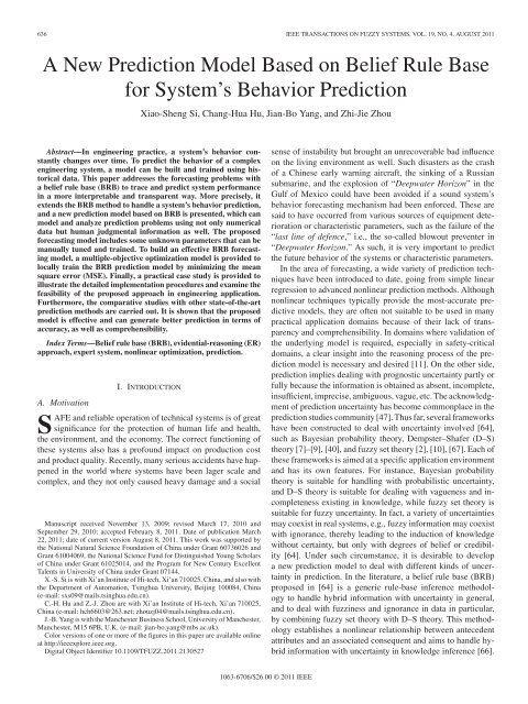
642 IEEE TRANSACTIONS ON FUZZY SYSTEMS, VOL. 19, NO. 4, AUGUST 2011ξ + j − ξ ∗ j > 0, j =1,...,N (17)where Q = {β j,k ,θ k ,δ i } is the training parameter vectorwith j =1,...,N,k =1,...,L,i=1,...,p, and ξ j (Q) is theMSE between the observed belief β j (t m ) and the predicted beliefˆβ j (t m ) by the BRB prediction model for the jth referentialterm. In this case, the optimization problem involves N objectivefunctions, L + L × N + p training parameters given as Qand L × N +2L + p constraints.In (14), φ j is the weighting parameter representing the relativeimportance of the jth objective function constrained with0 ≤ φ j ≤ 1 and ∑ Nj=1 φ j =1. In this paper, for simplicity,φ j is set to be equivalent for all objective functions, i.e.,φ j =(1/N ),j =1,...,N. ξ + j and ξj ∗ are the feasible maximumand minimum values for the jth objective function, asdefined in (15). It can be seen from (14) to (17) that the optimizedobjective is a function of parameter vector Q, while theelements of Q are constrained in the continuous region, as definedin (8)–(11). In this sense, we can see that β j,k ,θ k , and δ iare continuous variables, and there is no discrete variable optimizedin (14). As shown in (6) and (7), ˆβ j (t) is a function ofβ j,k ,θ k , and δ i , and thus, the optimized objective function canbe considered to be continuous. Therefore, such a minimax optimizationmodel can be solved using MATLAB optimizationtoolbox with FMINIMAX function. In addition, we note thatthis function FMINIMAX has been used for a similar purposein [28] and [66]. Once the input–output data become available,the related parameters to the BRB prediction model canbe obtained rationally. Then, the system’s behavior state can bepredicted when the new information becomes available.IV. DEMONSTRATION OF BELIEF-RULE-BASE PREDICTIONMODEL: APRACTICAL CASE STUDYIn this section, a practical case study is examined to validatethe BRB prediction model under the distributed outputs andto show the application potential of BRB prediction model inengineering practice.As a key device of INSs in weapon systems and space equipments,an inertial navigation platform plays an irreplaceableimportant role and its operating state has a direct influence onnavigation precision. In our tested inertial navigation platform,the sensors are fixed in it, which mainly include three DTGsand three accelerometers, measuring angular velocity and linearacceleration, respectively. Statistical analysis shows that almost80% failures of inertial platforms result from gyroscopic drift.In our case, the gyro fixed on an inertial platform is a mechanicalstructure having 2 degrees of freedom from the driver and senseaxis. For a general description of an inertial navigation platformand gyros, see [55]. When the inertial platform is operating,the rotating wheel of DTGs with very high speed can lead torotation axis wear, and finally, result in gyro’s drift. With accumulationof wear, the drift degrades, and finally, results in thefailure of DTGs. Especially, several fails in launching, which areresulted by the abnormality of the DTGs, are strongly drivingforces for building reliable and cost-effective prediction modelthat can provide the complete picture of the DTG by analyzingFig. 1.Entire gyroscopic drift data collected in the trial.the changing trend of the DTG drift. As such, the drift of DTGsis usually used as a performance indicator to evaluate the healthcondition of an inertial platform. Since such DTG is widely usedin aeronautic control system with safety-critical requirement, itis desired that the adopted model is not only comprehensible byhuman expert, but also transparent with inference process, andcan provide some explanations of the predicted results. As analyzedabove, the BRB prediction model can satisfy these desiresin the sense that it can provide a complete picture on the stateof DTG, such as the belief degree on each assessment grade.In our study, we only take the drift-degradation measurementalong the sense axis for an illustration purpose since this variableplays a dominant role in the assessment of gyros degradation.The demonstration of the proposed model is conducted in thefollowing and some comparative studies are provided as well.A. Problem DescriptionIn this study, the system’s drift data are collected in a DTGperformance reliability trial from leaving factory. For the DTGdrift trial, some technical parameters include the sampling intervalT , the acceleration of gravity g, and the geographic latitudeR. In this experiment, T =2.2 h, g = 979.4121 cm/s 2 ,and R =34.6006 ◦ , where a PC-based data-acquisition systemis used to acquire and store the drift data. After the experiment,we can collect all the drift data. The datasets include the timeto-driftdata for 90 suits of gyroscope. The experiment resultsare illustrated in Fig. 1.As shown in Fig. 1, it indicates that the gyroscopic drift isa time series. Therefore, it is reasonable to assume that thecurrent gyroscopic drift value y t is related to the most recenty t−1 , or even extended into the past values y t−2 ,...,y t−p .Thisis because the next gyroscopic drift value is dependent on thecurrent level of gyroscope state to a certain extent. As such, y t−ican be treated as the antecedent attributes of the rule base, wherei =1,...,p. In next section, the BRB prediction model will beestablished to predict the behavior of DTG at time t based ony t−1 ,y t−2 ,...,y t−p .

SI et al.: NEW PREDICTION MODEL BASED ON BELIEF RULE BASE FOR SYSTEM’S BEHAVIOR PREDICTION 643B. <strong>Prediction</strong> <strong>Model</strong> <strong>Based</strong> on the Belief-Rule-Base ApproachThe BRB system is used to capture the relationship amongy t−1 ,y t−2 ,...,y t−p through system state after p steps, whichcaptures the dynamics of DTG. This kind of BRB system canbe considered as the forecasting model and used to predict thefuture behavior of the system. Thus, the prediction BRB systemcan be constructed as follows:R k : IF y t−1 is A k 1 ∧ y t−2 is A k 2 ···∧y t−p is A k p , THENsystem state at next step is {(D 1 ,β 1,k ),...,(D N ,β N,k )}with a rule weight θ k and attribute weight δ 1 ,δ 2 ,...,δ p .For simplicity, this study experimented with a relatively smallernumber p, and then, two antecedent attributes are selected as anexample. Consequently, we can transform 90 observed valuesto 88 sets of input–output patterns according Table I. Then, thebelief rule can be represented as follows:R k : IF y t−1 is A k 1 ∧ y t−2 is A k 2 , THEN system stateat next step is {(D 1 ,β 1,k ),...,(D N ,β N,k )} with arule weight θ k and attribute weight δ 1 ,δ 2 ,...,δ pwhere R k (k =1,...,L) is the belief rules of the BRB. In theBRB, A k 1 and A k 2 are the referential points of y t−1 and y t−2 ,respectively. D l (l =1,...,N) are the assessment grades ofsystem’s behavior.C. Referential Points of the Antecedents and ConsequenceFrom Fig. 1, we can see that the original input data wereall provided as numerical numbers; therefore, there is a needto equivalently transform the numerical value into the beliefstructures. Note that the referential values of an attribute andthe types of input information are problem specific [26], [59].In this case study, the technical requirement of DTG is that thedrift value is not larger than 2.4 ◦ h −1 ; therefore, the linguisticlabels for y t−1 ,y t−2 are defined as “Small”(S), “Medium”(M),and “Large” (L). i.e., A k i ∈{S, M, L} for i =1and 2. Forthesystem’s behavior state, three assessment grades of system’sbehavior for outputs of BRB prediction system are used, andthey are “Good” (G), “Average” (A), and “Poor” (P ); this isto say that D =(D 1 ,D 2 ,D 3 )=(G, A, P ). As such, in ruleR k (k =1,...,L) in above section, L =9and N =3.The referential points of inputs defined above are in linguisticterms and need to be quantified. In [62], a scheme to convertother inputs to belief structure has been developed. In theproposed scheme, there is an important technique, i.e., rulebasedinformation-transformation technique, which is used todeal with the input/output information involving quantitativedata. After data transformation, quantitative data can be transformedto belief structures, and the two are equivalent in thesense that they both represent the same states of the system. Formore details, see [62]. The quantified results in this case studyare listed in Table II.D. Simulation Results Under Belief Distribution OutputTo validate the BRB prediction model, the available data arepartitioned into a training dataset and a testing dataset. The trainingdataset is used to train the BRB-prediction-model parameters.In this case, the output is transformed into the followingdistributed output format:S(output) ={(D 1 ,β 1 ), (D 2 ,β 2 ), (D 3 ,β 3 )}where β i ,i=1, 2, and 3 can be obtained by the rule-basedinformationtransformation. Since the gyroscopic drift is a timeseries and the input–output patterns are constructed by Table I,we use the same referential points as given in Table II for theassessment grades of system’s behavior D i ,i=1, 2, and 3,respectively.As such, according to Table II, one of transformationrules for system-assessment grade D 1 could be read as follows:If gyroscopic drift is 1.0 ◦ h −1 , then system’s behavior state isranked to be “Good” with the matched degree 1.0, i.e., D 1 =1.0.The other two transformation rules can be interpreted in a similarway. For instance, using the defined referential points, the35th data with output value 1.28 ◦ h −1 in our dataset can be transformedinto S(output) = {(D 1 ,0.7),(D 2 ,0.3),(D 3 ,0)} based onrule-based transformation technique. Similar to the example inSection II-C, we have β 1 =(1.4 − 1.28)/(1.4 − 1) = 0.3, andβ 2 =(1.28 − 1)/(1.4 − 1) = 0.7. In fact, this process is similarto fuzzification step used in fuzzy set theory [2], [10]. However,it is worth noting that the referential values used in the aboverules are problem-dependent. In our case study, it is usually requiredthat the drift of the DTG is not larger than 2.4 ◦ h −1 sincethe DTG is used in a safety-critical system.In this case study, three BRB prediction systems are constructedfor this validation analysis. The first BRB is directlyconstructed from expert knowledge about the relationship betweensystem’s behavior and drift, which simulated the uncertaininformation in system’s behavior prediction. The secondBRB is given by an engineering practitioner. Then, it is trainedusing the proposed optimization method and the data are generatedfrom the first BRB, thus leading to the third optimallytrained BRB. Finally, the trained BRB prediction model is usedto predict outputs for the testing input data. In order to make ourfollowing listed steps clear, we select the 35th data used in ourdataset to illustrate and track the changes in each step.1) Step 1: Directly Construct a Benchmark Belief Rule BaseAccording to the Prior Knowledge: In engineering practice, theDTG drift values change over time, as shown in Fig. 1. The inertialsystem presents great requirement to the precision of DTG.In practice, DTG drift as an indication of performance of DTGis the smaller the better, i.e., if the drift value is large, then thebehavior of DTG can be assessed to “Poor” with great possibility.<strong>Based</strong> on this principle, a benchmark BRB is constructedthrough expert intervention, as shown in Table III.In the benchmark BRB, the values of θ k and δ i are all set to1, where k =1,...,9, and i =1,...,2, except θ 3 ,θ 5 , and θ 7 .For example, the value of θ 3 is 0.9, which is less than 1.0, whichrepresents that the rule 3 has a low credibility. To some extent,this reflects the knowledge that we have obtained is not completeand some uncertainties exist in assessment results. This BRBis used as a benchmark to check how closely a BRB, whichis initialized either using historical or using expert knowledge,can be trained using the proposed training algorithm to simulate

644 IEEE TRANSACTIONS ON FUZZY SYSTEMS, VOL. 19, NO. 4, AUGUST 2011TABLE IIIBENCHMARK BRB PREDICTION SYSTEMthe true relationship. Therefore, the BRB shown in Table III isreferred to as benchmark BRB for short.To apply the benchmark BRB to construct the benchmarkdistributed outputs, the input values of y t−1 and y t−2 alsoneed to be transformed and represented in terms of the referentialvalues in the form of A k i ∈{S, M, L}. Then, (6) and(7) are used to generate the distributed outputs of the benchmarkBRB, as defined in Table III. The generated distributedoutputs are then used to be the true behavior state for thebenchmark distributed outputs. Since the inputs data of the 35thdata used in our dataset has been converted into the requiredbelief structure, the output of the benchmark BRB predictionsystem for this data point can be computed by (6) and (7) as{(D 1 , 0.749) , (D 2 , 0.1425) , (D 3 , 0.1085)}. Other data can beobtained in a similar way. The distributed outputs of the benchmarkBRB are shown graphically in Fig. 2(a)–(c).2) Step 2: Set the Parameters of the Initial Belief Rule Base:The belief degrees in the initial BRB are given and listed inTable IV. The initial values of θ k and δ i are all set to 1, where k =1,...,9, and i =1and 2. The initial belief degrees in Table IVare determined by the expert knowledge according to the runningpatterns and historical data of the DTG and the change of thedrift values over time. For example, according to the historicalinformation, if y t−1 is “Small” and y t−2 is “Small,” the expertjudges that the possibility of system in the “Good” state islarger than the other states. Therefore, the expert may assessthat the belief degree to “Good” is 0.95 and the belief degreeto “Average” is 0.05 and to “Poor” is 0, respectively. Thus, theinitial belief rule can be obtained as the second row of Table IV.The other rules can be initialized in a similar way.Once the initial BRB prediction system is constructed, it canbe used to predict the system’s behavior. For illustration purposes,all sets of sampling data are used for testing the performanceof the initial BRB. As shown in Fig. 2(a)–(c), we canobserve that the belief degrees to the consequents calculated by(6) and (7) using the initial BRB do not match well the distributedoutputs generated by the benchmark BRB, as defined inTable III. Similar to step 1, the output of the initial BRB predictionsystem for the 35th data can be computed by (6) and (7) as{(D 1 , 0.8579) , (D 2 , 0.1106) , (D 3 , 0.0314)}. Obviously, thereare significant difference between the output of the benchmarkBRB and the initial BRB. This means that the initial rule baseFig. 2. Predicted results of BRB prediction model being (a) “good,”(b) “average,” and (c) “poor.”provided by the expert is not good enough. Therefore, it is necessaryto use the available information to train the rule base bythe optimization approach.

SI et al.: NEW PREDICTION MODEL BASED ON BELIEF RULE BASE FOR SYSTEM’S BEHAVIOR PREDICTION 645TABLE IVINITIAL BRB PREDICTION SYSTEMTABLE VTRAINED BRB PREDICTION SYSTEM3) Step 3: Train the Belief Rule Base Constructed Initiallyin Step 2: After the input values y t−1 and y t−2 are transformedand represented in terms of referential values, based on the datagenerated for construction of the benchmark BRB, as shown instep 1, and the initial BRB, as given by the expert in step 2, theoptimization models (14)–(17) are used to train the initial BRB.For illustration purposes, the first 50 sets of data are used as thetraining data for parameter estimation. In this simulation, theerror tolerance is set to 0.05 and the maximum iteration is setto 100 to avoid dead loop in the optimal learning process. Thetrained results are listed in Table V.After training, the remaining 38 sets of data are used fortesting the trained BRB prediction model. The test results areillustrated in Fig. 2(a)–(c), where the comparisons are shownbetween the actual output and the predicted output that is generatedusing the trained BRB prediction model and the initial one.It is clear that the distributed outputs generated by the trainedBRB system can match the benchmark BRB more closely thanthe initial BRB. Similar to the previous two steps, the outputof the trained BRB prediction system for the 35th data can beobtained as {(D 1 , 0.7748) , (D 2 , 0.1407) , (D 3 , 0.1145)}. Thisfurther demonstrates that the trained BRB can match the benchmarkBRB accurately and the established optimization methodcan work well.As discussed in Section I, we can see that probabilistic interpretationis possible in our case here since the belief degree isonly assigned to the single grade of the assessment framework inthe BRB model. This result arises from rule-based transformationtechnique and ER algorithm. Therefore, we can considerbelief degree as a generalized probability from either Dempster’slower and upper probability [7]–[9] or Smets’ pignisticprobability [41] viewpoints. In the following, we can give aclear interpretation of the predicted outputs and assessed results.Taking the predicted curve being grade “Good” [see Fig. 2(a)],for example, we can read from probabilistic viewpoint that theprobability of DTG system’s behavior assigned to grade “Good”increases from 0.1998 to 0.724 monotonously and then experiencesa fluctuating process around 0.72. The reason that thebelief degree assigned to grade “Good” is below 0.5 in the firstseven sampling period lies in the fact that this kind of DTG isnot stable at the beginning of its operating time. As shown inFig. 2(a), the belief degree assigned to grade “Good” is around0.72 with the steady operation of DTG system, i.e., the functionof DTG is good almost with the probability value 0.72. Atthe same time, the probability of system’s behavior assignedto grade “Poor” is small. The other cases can be analyzed in asimilar way. From the above analysis, we can conclude that thefunction and behavior of DTG is normal in this case and that theproposed method can give complete picture about the operatingstate of DTG. These results can provide valuable informationfor conducting cost-effective maintenance and avoiding a largecalamity.4) Step 4: Performance Evaluation: In this section, the resultsof predicted results using BRB prediction model will bediscussed. The histograms of the absolute difference betweenthe actual and the predicted by the initial BRB and the trainedBRB are shown in Fig. 3.It can be seen that the absolute errors of most of samplesusing trained BRB are less than 0.01 in terms of assessment“Good,” as shown in Fig. 3(b), when compared with the rangeof the predicted results in Fig. 2(a). For the predicted values interms of assessment “Average” and “Poor,” the histograms ofthe absolute errors are shown in Fig. 3(b). All predicted resultsof trained BRB model are acceptable. In contrast, the absoluteerrors of most of samples using the initial BRB model are closeto 0.1 in terms of assessment “Good,” as shown in Fig. 3(a).In order to further demonstrate the proposed method, fivemeasures of forecasting performance are introduced [34],[45], [46], including mean absolute percentage error (MAPE),root MSE (RMSE), Teil’s inequality coefficient (TIC), Teil’sU-statistics (TUS), and modeling efficiency (ME). These indicatorsare all based on forecast residuals and are widely employedin the realm of forecasting practice. The detailed mathematicalexpressions are summarized in Table VI. The measures MAPEand RMSE have been widely used in prediction field to testthe accuracy of the prediction model [6], [22], [24], [54], [56],where RMSE can, in part, measure the variance character inpredicted results. Here, we report on additional measures TIC,TUS, and ME since they provide some simple performances onrelative scale that can avoid the scaling problem of both MAPEand RMSE. If TIC = 0orTUS= 0, then the model produces

646 IEEE TRANSACTIONS ON FUZZY SYSTEMS, VOL. 19, NO. 4, AUGUST 2011Fig. 3Histogram of absolute difference by (a) initial BRB, (b) trained BRB, (c) BRF neural networks, (d) ARMA/GARCH, (e) FCM-TS model, and (f) LSSVM.perfect predictions. In addition, ME = 1 indicates a perfect fit,ME = 0 reveals that the model is no better than a simple average,and ME < 0 indicates a poor forecasting performance.In this case study, the above measures are used to evaluatethe prediction performance. For example, the MAPE and MEbetween the benchmark BRB and the initial BRB in terms beliefdegrees to the linguistic term “Good” is 0.1923 and 0.0475, respectively.However, after training prediction model, the MAPEand ME in terms of the belief degrees to “Good” are 0.003 and0.9935, respectively. This provides the evidence for the validity

SI et al.: NEW PREDICTION MODEL BASED ON BELIEF RULE BASE FOR SYSTEM’S BEHAVIOR PREDICTION 647TABLE VISTATISTICAL MEASURES OF PREDICTION ACCURACYTABLE VIIPERFORMANCE OF DIFFERENT MODELS USING THE SAME DTG-TESTING DATASETof the developed prediction model and optimization methodsince the MAPE value is smaller and the ME value is very closeto 1. The detailed results are listed in Table VII.<strong>Based</strong> on the above experiment results, it is clear that theinitial belief rules for system’s behavior prediction given by anexpert are not accurate. When the running information of systembecomes available, the proposed optimization model can trainthe BRB effectively.E. Comparative StudiesWith the same dataset, we obtain the predicted results byARMA/GARCH [36], RBFNN [68], LSSVM [44], and FCM-TS models [23] as a comparison of the measure of the learningability of the proposed model. The histograms of the absolutedifference between the actual and the predicted using thesemethods are shown in Fig. 3(c)–(f), and Table VII lists the measuresof forecasting performance. Even though the performanceof ARMA/GARCH, RBFNN, LSSVM, and FCM-TS predictorcould be improved by optimizing the related parameters,it is clear that the proposed BRB predictor performs the best.The predicted results of the DTG behavior on testing datasetby these methods are shown in Fig. 4(a)–(c). It is worth noting,from Fig. 4(a), that both the proposed method and FCM-TSpredictor generate better prediction on grade “Good” than othermethods to some extent. However, under the same condition,our method can perform better on grades “Average” and “Poor”than the FCM-TS predictor, as shown in Fig. 4(b) and (c). Inaddition, the measures presented in Table VII further supportthis point.In experiment, it should be noted that even though the BRBprediction model takes a little longer time (i.e., 6.21 s) in trainingthan other predictors, it is still an effective tool in DTG-behaviorforecasting application. The reasons are twofold. First, the samplinginterval is about 2.2 h in DTG-monitoring process. Accordingly,the average training speed of 6.21 s still means aneffective processing speed in this case study. Moreover, in mostreal-world applications, the time interval between two samplesis usually in terms of hour(s) or day(s); hence, the model developedin this paper can perform well in real-world forecastingpractice. Second, in contrast with real-time requirement in DTGbehaviorprediction, safety and interpretability are more desireddue to its safety-critical requirement in application. To furtherreveal the improvement of the proposed model, we have a lookat the aspect of interpretability of the used models above. Here,the ARMA/GARCH, RBFNN, LSSVM, and FCM-TS predictorare used to show the learning ability of the BRB model.Therefore, the same training and testing datasets are used forARMA/GARCH, RBFNN, LSSVM, FCM-TS, and BRN predictors.However, if we do not use the rule-based transformationtechnique under ER and BRB framework, the dataset cannot beconverted into the belief structures, and thus, ARMA/GARCH,

648 IEEE TRANSACTIONS ON FUZZY SYSTEMS, VOL. 19, NO. 4, AUGUST 2011and the performance of LSSVM is heavily dependent on σ, ε,and C, but they are difficult to select [44]. Unlike these models,the parameters in BRB have clear meaning. For example, in thesecond rule of Table V, the trained rule weight is 0.9475, whichreflects the credibility of this rule, and the estimated results inconsequent part can also reflect a complete picture of the system’sbehavior. The interpretability of such structure has beenillustrated in Sections I and IV-D. This contrasts sharply withARMA/GARCH, RBFNN, LSSVM, and FCM-TS predictors ifwe do not model prediction problem under the ER and BRBframework.Fig. 4. Predicted results on testing dataset being (a) “good,” (b) “average,”and (c) “poor.”RBFNN, LSSVM, and FCM-TS predictors can neither directlydeal with the inputs with belief structures nor generate the outputswith the belief structures as BRB model. However, theoutputs with the belief structures are easy to interpret, as shownin Section IV-D. In addition, the parameters in ARMA/GARCH,RBFNN, LSSVM, and FCM-TS are difficult to interpret. For example,the connection weights of RBFNN are not easy to explainF. Effect of the Number of Linguistic Labelsin Antecedent on the Predicted ResultsThe number of linguistic labels determines granularity of thelinguistic representation with respect to the numerical values. Inforegoing simulation studies, a three-label set in antecedent andconsequence is chosen as an example. Certainly, other choicescan be used as well, but the final judgment will be based onthe goodness-of-fit testing and the specific requirements in engineeringapplications. Therefore, the selection of the labels ofthe antecedent and consequence is problem-dependent. In thefollowing, we give a simulation study to show the effect of thenumber of labels set in antecedent on the prediction results. Theeffect of the consequent partition can be analyzed in a similarway and, thus, is omitted due to limited space.As a matter of fact, more label sets in prediction model meansthat there are more number of belief rules in BRB system sincethe relationship between the label set of antecedent and thenumber of belief rules can be written as L = ∏ pi=1 J i.Ifallantecedent attributes share the same number of referential valueJ, as in this paper, then the numbers of belief rule can be writtenas L = J p . Under such case, the processed problem can berepresented more specifically. However, the increase of beliefrule will cause that more unknown parameters need to be optimizedsince the number of unknown parameters is calculated byL + L × N + p. In addition, the more labels we use, the lowerthe interpretability of the model. In order to show the effect ofthe number of label sets in antecedent on the predicted results,a simulation is given under different numbers of antecedents asin the following. Specifically, four-label, six-label, and ten-labelsets are used to show the impact of the number of the labels on thepredicted result. It corresponds to BRB prediction model having16 rules, 36 rules, and 100 rules, respectively. In the simulation,the initial parameters of BRB are assigned randomly with constraints(8)–(11). In the obtained results, the MAPE fluctuatesalong with increasing number of labels—0.2% for four labels,0.21% for six labels, and 0.18% for ten labels. However, theME increases correspondingly—0.9955 for four labels, 0.9957for six labels, and 0.9959 for ten labels. Table VIII shows theinfluence of the number of linguistic labels on the predictedresults.From Table VIII, we can see that the prediction accuracycan be improved for a greater label set in antecedent, but theimprovement is a bit small in this simulation. A possible explanationfor this is that when increasing the number of labels,

SI et al.: NEW PREDICTION MODEL BASED ON BELIEF RULE BASE FOR SYSTEM’S BEHAVIOR PREDICTION 649TABLE VIIIPERFORMANCE EVALUATION UNDER DIFFERENT NUMBER OF LABEL SETthe number of belief rules increases correspondingly, e.g., 16,36, and 100 for 4, 6, and 10 labels, respectively. However, theincreased belief rules do not influence the predicted value asheavily, since many of belief rules cannot be activated by the inputdata. We also note that more time is needed to train the BRBprediction model for a greater label set and the average trainingtime increases as well. The reason for such an unexpected caseis that the number of belief rules increases as analyzed above.These results show that we cannot choose BRB arbitrarily sincemore time is needed to train the BRB prediction model for agreater label set and the interpretability of the model can belowered for a greater label set. In this case study, a three-labelset is a tradeoff between the prediction accuracy and trainingefficiency. The issues associated with how to select the numberof the label set may be considered in further research.G. Discussion<strong>Based</strong> on the above experiments, it is clear that the initialbelief rules for system’s behavior prediction given by an expertare not accurate. With the accumulation of the new knowledgeor input–output data, the proposed prediction model can beprogressively trained to better simulate a real system. Once theBRB prediction is trained, its knowledge can be used to forecastfuture behavior. However, as known for rule-base system, thereare some typical types of structural errors including conflictrules, missing rules, redundant rules, and circular dependingrules [16], [33]. It is noted that the prediction model, in thispaper, are initially built using expert knowledge or historicaldata, and then tuned by optimization. Hence, they are not yetequipped with the ability to automatically identify and rectifyconflicting rules. If conflicting rules are identified by experts orcertain relationships among rules are required, then additionalconstraints could be added to the optimization models to avoidconflicts and to meet the requirements. On the other side, for acomplex real-world problem, prior knowledge may be limited,which may lead to the construction of an incomplete, or eveninappropriate, initial BRB structure. If there are too many beliefrules in an initial rule base, the training task may become toocomplicated to handle, or it is possible to result in overfitting. Forexample, in this paper, we consider all possible rules, but rules 3and 7 in Table V were not trained at all as the belief degrees andrules weights of these rules remain unchanged after the training,as marked in gray in Section IV-D. However, in practice, whenactivated, such rules that are untouched during training maylead to an irrational conclusion if they were initially assignedrandomly or without care. If there are too few rules in the initialrule base, this may lead to underfitting. To achieve an overalloptimal BRB prediction model, however, the structure of a BRBsystem may need to be adjusted and optimized as well. Thisinvolves parameters identification and structure identificationsimultaneously. In fact, there are some good papers addressingoptimal design of the rule-based system, such as rule-reductionor rule-simplification techniques in fuzzy-rule-base literature[13], [14], [39], as discussed previously. In this paper, we donot consider such issues; however, the above simulation resultsindeed suggest that considering the optimal design of the BRBsystem is necessary and valuable in future work. This can alsoimprove the interpretability of the model since the unknownparameters may be reduced. One thing that is worth noting isthat the measure variance accounted for (VAF) [12], [35] maybe useful for quantifying the improvement of the optimizedmodel in the case when the optimal design of the BRB is takeninto account, since the VAF can measure the predictor variableimportance. This is valuable for further research as well.V. CONCLUSIONThis paper addresses the forecasting problems with BRBto improve the interpretability of the predicted result. Moreprecisely, it extends BRB to handle system’s behavior predictionproblem, and a new prediction model based on BRB ispresented, which can model and analyze prediction problemsusing not only numerical data but human judgmental informationas well. In order to build an effective BRB forecastingmodel, a multiple-objective optimization model is providedto locally train the BRB prediction model by minimizing theMSE criterion. Finally, a practical study is provided to illustratethe detailed implementation procedures of the proposedapproach and examine the feasibility and validity in real-lifebehavior prediction of DTG used in the INS. Compared withARMA/GARCH, RBFNN, LSSVM, and FCM-TS predictors,the proposed method is superior in terms of prediction accuracyand interpretability; hence, it can be regarded as an effectivetool for prediction applications.There are three features in the proposed model that are inheritedfrom BRB system. First, the BRB prediction modelprovides a powerful simulator that can explicitly represent expert’sdomain-specific knowledge as well as common-sensejudgments and, thus, can avoid generating obviously irrationalconclusions. Second, the new model is capable of processing inputand output information that can be numerical or distributed

650 IEEE TRANSACTIONS ON FUZZY SYSTEMS, VOL. 19, NO. 4, AUGUST 2011with an information-transformation technique, thereby providinga flexible way to represent and deal with hybrid informationencountered in forecasting practice. Third, the BRB predictionmodel is designed to allow the direct intervention of experts indeciding the internal structure of a belief rule and is comprehensibleto humans in aspects of model parameter as well asprediction results from a probabilistic point of view. In furtherresearch, we will consider the optimal design of the BRB modeland the online parameter-estimation methods for the proposedmodel.ACKNOWLEDGMENTThe authors would like to sincerely thank and acknowledgethe tremendous work and the inputs performed by the AssociateEditor and the three anonymous reviewers for their valuablesuggestions and thorough review, which have greatly improvedthis paper. Particularly, they would like to thank one anonymousreviewer for his/her insightful comments, which have improvedthe representation significantly.REFERENCES[1] C. Angeli and A. Chatzinikolaou, “<strong>Prediction</strong> and diagnosis of faults inhydraulic systems,” Proc. Inst. Mech. Eng., vol. 216, no. 2, pp. 293–297,2002.[2] R. Babuska, Fuzzy <strong>Model</strong>ing for Control. Boston, MA: Kluwer, 1998.[3] M. Z. Chen, D. H. Zhou, and G. P. Liu, “A new particle predictor for faultprediction of nonlinear time-varying systems,” Developments ChemicalEng. Mineral Process., vol. 13, no. 3/4, pp. 379–388, 2005.[4] W. T. Chen and M. Saif, “A novel fuzzy system with dynamic rule base,”IEEE Trans. Fuzzy Syst., vol. 13, no. 5, pp. 569–582, Oct. 2005.[5] K. Y. Chen, “Forecasting system’s reliability based on support vectorregression with genetic algorithms,” Rel. Eng. Syst. Safety, vol. 92, no. 4,pp. 423–432, 2007.[6] L. H. Chen and C. C. Hsueh, “Fuzzy regression models using the leastsquaresmethod based on the concept of distance,” IEEE Trans. FuzzySyst., vol. 17, no. 6, pp. 1259–1272, Dec. 2009.[7] A. P. Dempster, “Upper and lower probabilities induced by a multivaluedmapping,” Ann. Math. Stat., vol. 38, no. 2, pp. 325–339, 1967.[8] A. P. Dempster, “A generalization of Bayesian inference,” J. Royal Stat.Soc., Series B, vol. 30, no. 2, pp. 205–247, 1968.[9] A. P. Dempster, “The Dempster–Shafer calculus for statisticians,” Int. J.Approx. Reason., vol. 48, no. 2, pp. 365–377, 2008.[10] J. M. de Costa Sousa and U. Kaymak, Fuzzy Decision Making in <strong>Model</strong>ingand Control (World Sci. Series Robotics Intell. Syst., vol. 27). RiverEdge, NJ: World Scientific, 2002.[11] W. Duch, R. Setiono, and J. M. Zurada, “Computational intelligencemethods for rule-based data understanding,” Proc. IEEE, vol. 92, no. 5,pp. 771–805, May 2004.[12] P. E. Green, J. Douglas, and W. S. Desarbo, “A new measure of predictorvariable importance in multiple regression,” J. Market. Res., vol. 15, no. 3,pp. 356–360, 1978.[13] S. Guillaume, “Designing fuzzy inference systems from data: Aninterpretability-oriented review,” IEEE Trans. Fuzzy Syst., vol. 9, no. 3,pp. 426–443, Jun. 2001.[14] S. Guillaume and B. Charnomordic, “Generating an interpretable familyof fuzzy partitions from data,” IEEE Trans. Fuzzy Syst., vol. 12, no. 3,pp. 324–335, Jun. 2004.[15] Y. Halpern and R. Fagin, “Two views of belief: Belief as generalizedprobability and belief as evidence,” Artif. Intell., vol. 54, no. 3, pp. 275–317, 1992.[16] X. D. He, W. L. C. Chu, and H. J. Yang, “A new approach to verifyrule-based systems using Petri nets,” Inf. Software Technol., vol. 45,pp. 663–669, 2003.[17] L. J. Herrera, H. Pomares, I. Rojas, O. Valenzuela, and A. Prieto, “Tase,a Taylor series-based fuzzy system model that combines interpretabilityand accuracy,” Fuzzy Sets Syst., vol. 153, pp. 403–427, 2005.[18] S. L. Ho and M. Xie, “The use of ARIMA models for reliability forecastingand analysis,” Comput. Ind. Eng., vol. 35, no. 1/2, pp. 213–216, 1998.[19] C. H. Hu, X. S. Si, and J. B. Yang, “System reliability prediction modelbased on evidential reasoning algorithm with nonlinear optimization,”Expert Syst. Appl., vol. 37, no. 3, pp. 2550–2562, 2010.[20] C. L. Huang and K. Yong, Multiple Attribute Decision Making Methodsand Applications, a State-of Art Survey. Berlin, Germany: Springer-Verlag, 1981.[21] Y. Q. Jiang, “Applying grey forecasting to predicting the operating energyperformance of air cooled water chillers,” Int. J. Refrigeration, vol. 27,no. 4, pp. 385–392, 2004.[22] C. F. Juang and C. D. Hsieh, “A locally recurrent fuzzy neural networkwith support vector regression for dynamic system modeling,” IEEETrans. Fuzzy Syst., vol. 18, no. 2, pp. 261–273, Apr. 2010.[23] E. Kim, M. Park, S. Ji, and M. Park, “A new approach to fuzzy modeling,”IEEE Trans. Fuzzy Syst., vol. 5, no. 3, pp. 328–337, Aug. 1997.[24] L. W. Lee, L. H. Wang, S. M. Chen, and Y. H. Leu, “Handling forecastingproblems based on two-factors high-order fuzzy time series,” IEEE Trans.Fuzzy Syst., vol. 14, no. 3, pp. 468–477, Jun. 2006.[25] G. D. Li, S. Masuda, D. Yamaguchi, and M. Nagai, “A new reliabilityprediction model in manufacturing systems,” IEEE Trans. Rel., vol. 59,no. 1, pp. 170–177, Mar. 2010.[26] J. Liu, J. B. Yang, H. S. Sii, and Y. M. Wang, “Fuzzy rule-based evidentialreasoning approach for safety analysis,” Int. J. Gen. Syst., vol. 33, no. 2/3,pp. 183–204, 2004.[27] J. Liu, J. B. Yang, and H. S. Sii, “Engineering system safety analysis andsynthesis using fuzzy rule based evidential reasoning approach,” QualityRel. Eng. Int., vol. 21, no. 4, pp. 387–411, 2005.[28] J. Liu, J. B. Yang, D. Ruan, L. Martinez, and J. Wang, “Self-tuning offuzzy belief rule bases for engineering system safety analysis,” Ann.Operational Res., vol. 163, pp. 143–168, 2008.[29] E. D. Lughofer, “FLEXFIS: A robust incremental learning approach forevolving Takagi–Sugeno fuzzy models,” IEEE Trans. Fuzzy Syst., vol. 16,no. 6, pp. 1393–1410, Dec. 2008.[30] R. T. Marler and J. S. Arora, “Survey of multi-objective optimizationmethods for engineering,” Struct. Multidiscip. Optim., vol. 26, pp. 369–395, 2004.[31] K. Miettine, Nonlinear Multiobjective Optimization. Boston, MA:Kluwer, 1999.[32] D. L. Nazareth, “Issues in the verification of knowledge in rule-basedsystems,” Int. J. Man–Mach. Stud., vol. 30, pp. 255–271, 1989.[33] G. Niu and B. S. Yang, “Dempster–Shafer regression for multi-step-aheadtime-series prediction towards data-driven machinery prognosis,” Mech.Syst. Signal Process., vol. 23, pp. 740–751, 2009.[34] N. Ogris and M. Jurc, “Sanitary felling of Norway spruce due to sprucebark beetles in Slovenia: A model and projection for various climatechange scenarios,” Ecol. <strong>Model</strong>., vol. 221, no. 2, pp. 290–302, 2010.[35] R. A. Peterson, “A meta-analysis of variance accounted for and factorloadings in exploratory factor analysis,” Marketing Lett., vol. 11, no. 3,pp. 261–275, 2000.[36] H. T. Pham and B. S. Yang, “Estimation and forecasting of machine healthcondition using ARMA/GARCH model,” Mech. Syst. Signal Process.,vol. 24, pp. 546–558, 2010.[37] E. A. Rietman and M. Beachy, “A study on failure prediction in a plasmareactor,” IEEE Trans. Semicond. Manuf., vol. 11, no. 4, pp. 670–680,Nov. 1998.[38] M. J. Roemer, C. S. Byington, G. J. Kacprzynski, and G. Vachtevanos,“An overview of selected prognostic technologies with reference to anintegrated PHM architecture,” in Proc. IEEE Aerosp. Conf.,BigSky,MT,2005.[39] M. Setnes, R. Babuska, U. Kaymak, and H. R. van Nauta Lemke, “Similaritymeasures in fuzzy rule base simplification,” IEEE Trans. Syst.,Man, Cybern., B, Cybern., vol. 28, no. 3, pp. 376–386, Jun. 1998.[40] G. Shafer, A Mathematical Theory of Evidence. Princeton, NJ: PrincetonUniv. Press, 1976.[41] P. Smets and R. Kennes, “The transferable belief model,” Artif. Intell.,vol. 66, no. 2, pp. 191–243, 1994.[42] W. Stach, L. Kurgan, and W. Pedrycz, “Numerical and linguistic predictionof time series with the use of fuzzy cognitive maps,” IEEE Trans. FuzzySyst., vol. 16, no. 1, pp. 61–72, Feb. 2008.[43] R. Sun, “Robust reasoning: Integrating rule-based and similarity-basedreasoning,” Artif. Intell., vol. 75, no. 2, pp. 241–295, 1995.[44] J. A. K. Suykens, T. van Gestel, J. De Brabanter, B. De Moor, andJ. Vandewalle, Least Support Vector Machines. Singapore: World Scientific,2002.

SI et al.: NEW PREDICTION MODEL BASED ON BELIEF RULE BASE FOR SYSTEM’S BEHAVIOR PREDICTION 651[45] H. Theil, Economic Forecast and Policy. Amsterdam, the Netherlands:North-Holland, 1961, p. 567.[46] L. Trapani and G. Urga, “Optimal forecasting with heterogeneous panels:A Monte Carlo study,” Int. J. Forecasting, vol. 25, pp. 567–586, 2007.[47] M. B. A. van Asselt, J. Mesman, and S. A. van’t Klooster, “Dealing withprognostic uncertainty,” Futures, vol. 39, no. 6, pp. 669–684, 2007.[48] J. van den Berg, U. Kaymak, and W.-M. van den Bergh, “Financial marketsanalysis by using a probabilistic fuzzy modelling approach,” Int. J.Approx. Reason., vol. 35, pp. 291–305, 2004.[49] P. Walley, “Measures of uncertainty in expert system,” Artif. Intell.,vol. 83, no. 1, pp. 1–58, 1996.[50] D. Wang, D. H. Zhou, Y. H. Jin, and S. J. Qin, “A strong tracking predictorfor nonlinear processes with input time delay,” Comput. Chem. Eng.,vol. 28, no. 12, pp. 2523–2540, 2004.[51] Y. M. Wang, J. B. Yang, and D. L. Xu, “Environmental impact assessmentusing the evidential reasoning approach,” Eur. J. Operational Res.,vol. 174, no. 3, pp. 1885–1913, 2006.[52] W. Wang, “An adaptive predictor for dynamic systems forecasting,” Mech.Syst. Signal Process., vol. 21, pp. 809–823, 2007.[53] Y. M. Wang, J. B. Yang, D. L. Xu, and K. S. Chin, “The evidentialreasoning approach for multiple attribute decision analysis using intervalbelief degrees,” Eur. J. Operational Res., vol. 175, no. 1, pp. 35–66, 2008.[54] W. Wang and J. Vrbanek, “An evolving fuzzy predictor for industrialapplications,” IEEE Trans. Fuzzy Syst., vol. 16, no. 6, pp. 1439–1449,Dec. 2008.[55] O. J. Woodman. (2007). An introduction to inertial navigation, Comput.Lab., Univ. Cambridge, Cambridge, MA, Tech. Rep. [Online]. Available:http://www.cl.cam.ac.uk/techreport/[56] D. Wang, X. J. Zeng, and J. A. Keane, “An evolving construction schemefor fuzzy systems,” IEEE Trans. Fuzzy Syst., vol. 18, no. 4, pp. 755–770,Aug. 2010.[57] K. Xu, M. Xie, L. C. Tang, and S. L. Ho, “Application of neural networksin forecasting engine systems reliability,” Appl. Soft Comput., vol.2,no. 4, pp. 255–268, 2003.[58] D. L. Xu, J. Liu, J. B. Yang, G. P. Liu, J. Wang, I. Jenkinson, and J. Ren,“Inference and learning methodology of belief-rule-based expert systemfor pipeline leak detection,” Expert Syst. with Appl., vol. 32, no. 1,pp. 103–113, 2007.[59] J. B. Yang and M. G. Singh, “An evidential reasoning approach for multipleattribute decision making with uncertainty,” IEEE Trans. Syst., Man,Cybern. A, Syst. Humans, vol. 24, no. 1, pp. 1–18, Jan. 1994.[60] S. K. Yang and T. S. Liu, “A Petri net approach to early failure detectionand isolation for preventive maintenance,” Qual. Rel. Eng. Int., vol. 14,no. 5, pp. 319–330, 1998.[61] S. K. Yang and T. S. Liu, “State estimation for predictive maintenanceusing Kalman filter,” Rel. Eng. Syst. Safety, vol. 66, no. 1, pp. 29–39,1999.[62] J. B. Yang, “Rule and utility based evidential reasoning approach formulti-attribute decision analysis under uncertainties,” Eur. J. OperationalRes., vol. 131, no. 1, pp. 31–61, 2001.[63] J. B. Yang and D. L. Xu, “On the evidential reasoning algorithm formultiple attribute decision analysis under uncertainty,” IEEE Trans. Syst.,Man, Cybern. A, Syst. Humans, vol. 32, no. 3, pp. 289–304, May 2002.[64] J. B. Yang, J. Liu, J. Wang, H. S. Sii, and H. W. Wang, “Belief rulebaseinference methodology using the evidential reasoning approach—RIMER,” IEEE Trans. Syst., Man, Cybern. A, Syst. Humans, vol. 36,no. 2, pp. 266–285, Mar. 2006.[65] J. B. Yang, Y. M. Wang, D. L. Xu, and K. S. Chin, “The evidential reasoningapproach for MADA under both probabilistic and fuzzy uncertainties,”Eur. J. Operational Res., vol. 171, no. 1, pp. 309–343, 2006.[66] J. B. Yang, J. Liu, D. L. Xu, J. Wang, and H. W. Wang, “Optimal learningmethod for training belief rule based systems,” IEEE Trans. Syst., Man,Cybern. Part A, Syst. Humans, vol. 37, no. 4, pp. 569–585, Jul. 2007.[67] L. Z. Zadeh, “Fuzzy sets,” Inform. Control, vol. 8, no. 3, pp. 338–353,1965.[68] A. S. Zhang and L. Zhang, “RBF neural networks for the prediction ofbuilding interference effects,” Comput. Struct., vol. 82, pp. 2333–2339,2004.[69] L. B. Zhang, Z. H. Wang, and S. X. Zhao, “Short-term fault prediction ofmechanical rotating parts on the basis of fuzzy-grey optimizing method,”Mech. Syst. Signal Process., vol. 21, pp. 856–865, 2007.[70] J. Zheng, “Predicting software reliability with neural network ensembles,”Expert Syst. Appl., vol. 36, pp. 2116–2122, 2009.[71] P. Zito, H. B. Chen, and M. C. Bell, “Predicting real-time roadside CO andNO2 concentrations using neural networks,” IEEE Trans. Intell. Transp.Syst., vol. 9, no. 3, pp. 514–522, Sep. 2008.Xiao-Sheng Si received the B.Eng. and M.Eng. degrees,all in control engineering, from the High-TechInstitute of Xi’an, Xi’an, China, in 2006 and 2009, respectively.He is currently working toward the Ph.D.degree with Tsinghua University, Beijing, China.He has authored or coauthored about 15 articlesin several journals including the European Journal ofOperational Research, the IEEE TRANSACTIONS ONSYSTEMS, MAN, AND CYBERNETICS PART A, ExpertSystems with Applications, Science China InformationSciences, etc. He has also been the Invited Reviewerfor several international journals. His current research interests includeevidence theory, expert systems, prognositics and health management, reliabilityestimation, predictive maintenance, and lifetime estimation.Chang-Hua Hu received the B.Eng. and M.Eng. degreesfrom the High-Tech Institute of Xi’an, Xi’an,China, in 1987 and 1990, respectively, and the Ph.D.degree from the Northwestern Polytechnic University,Xi’an, in 1996.He is currently a Professor with the High-TechInstitute of Xi’an. During September 2008–December 2008, he was a Visiting Scholar with theUniversity of Duisburg, Duisburg, Germany. His currentresearch was supported by the National ScienceFoundation of China. He has authored or coauthoredtwo books and about 100 articles. His current research interests include faultdiagnosis and prediction, life prognosis, and fault-tolerant control.Jian-Bo Yang received the B.Eng. and M.Eng. degreesfrom the Northwestern Polytechnic University,Xi’an, China, in 1981 and 1984, respectively, andthe Ph.D. degree in decision sciences and systemsengineering from Shanghai Jiao Tong University,Shanghai, China, in 1987.He is currently a Professor of decision and systemsciences and the Director of the Decision SciencesResearch Center, Manchester Business School, Universityof Manchester, Manchester, U.K. He is also aSpecially Appointed Changjian Chair Professor withthe School of Management, Hefei University of Technology, Hefei, China. Hewas a Faculty Member with the University of Manchester Institute of Scienceand Technology, in 1990 and again from 1998 and 2004, the University ofBirmingham, Birmingham, U.K., from 1995 to 1997, the University of <strong>New</strong>castleupon Tyne, <strong>New</strong>castle upon Tyne, U.K., from 1991 to 1995, and ShanghaiJiao Tong University, Shanghai, China, from 1987 to 1989. Over the past twodecades, he has been conducting research in multiple criteria decision analysisunder uncertainty, multiple-objective optimization, intelligent decision-supportsystems, hybrid quantitative and qualitative decision modeling using techniquesfrom operational research, artificial intelligence, and systems engineering, anddynamic system modeling, simulation, and control for engineering and managementsystems. His current research interests include design decision making, riskmodeling and analysis, production planning and scheduling, quality modelingand evaluation, supply-chain modeling and supplier assessment, and the integratedevaluation of products, systems, projects, policies, etc. He has authoredor coauthored three books, more than 140 papers in international journals/bookchapters, and a similar number of papers in conferences. He has developed severalsoftware packages in these areas, including the Windows-based intelligentdecision system via evidential reasoning.Zhi-Jie Zhou received the B.Eng. and M.Eng. degreesfrom the High-Tech Institute of Xi’an, Xi’an,China, in 2001 and 2004, respectively. He is currentlyworking toward the Ph.D. degree with Tsinghua University,Beijing, China.He is currently a Lecturer with the High-Tech Instituteof Xi’an. He was a Visiting Scholar with theUniversity of Manchester, Manchester, U.K., fromMarch to August 2009. He has authored or coauthoredabout 25 articles. His current research interestsinclude belief rule bases, dynamic system modeling,hybrid quantitative and qualitative decision modeling and fault prognosis, andoptimal maintenance of dynamic systems.