dset 1 1 1 stats.sb04.betas+tlrc

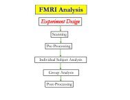
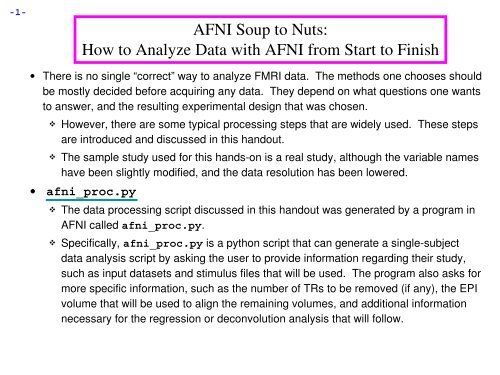
-1-AFNI Soup to Nuts:How to Analyze Data with AFNI from Start to Finish• There is no single “correct” way to analyze FMRI data. The methods one chooses shouldbe mostly decided before acquiring any data. They depend on what questions one wantsto answer, and the resulting experimental design that was chosen. However, there are some typical processing steps that are widely used. These stepsare introduced and discussed in this handout. The sample study used for this hands­on is a real study, although the variable nameshave been slightly modified, and the data resolution has been lowered.• afni_proc.py The data processing script discussed in this handout was generated by a program inAFNI called afni_proc.py. Specifically, afni_proc.py is a python script that can generate a single­subjectdata analysis script by asking the user to provide information regarding their study,such as input datasets and stimulus files that will be used. The program also asks formore specific information, such as the number of TRs to be removed (if any), the EPIvolume that will be used to align the remaining volumes, and additional informationnecessary for the regression or deconvolution analysis that will follow.

-2-At the moment, this information is input via a command­line interface, or with anoptional question/answer session (afni_proc.py -ask_me). Eventually, a GUIwill become available (but not yet). Once afni_proc.py has all the necessary information, it produces a tcsh (T­shell)script that contains all the data processing steps. This script can be easily executedand the end result will be a functional/statistical dataset, as well as numerous datasetsproduced from the intermediary steps.• Before we go any further, start the processing script : we will discuss it more, soon under AFNI_data4, execute the script containing the afni_proc.py commandthis will create the processing script, proc.sb23.blk execute the proc.sb23.blk script, as recommended by afni_proc.pytakes ~4 minutes on my laptopcd AFNI_data4tcsh s1.afni_proc.blocktcsh -x proc.sb23.blk |& tee output.proc.sb23.blk note that one could subsequently run s10.surface.analysis to analyze the data inthe surface domain (which takes ~37 minutes on my laptop)

-3-• The Experiment : Cognitive Task: Subjects see photographs of two people interacting.The mode of communication falls in one of 3 categories: via telephone, email, orface­to­face.The affect portrayed is either negative, positive, or neutral in nature. Experimental Design: 3x3 Factorial design, BLOCKED trialsFactor A: CATEGORY ­ (1) Telephone, (2) E­mail, (3) Face­to­FaceFactor B: AFFECT ­ (1) Negative, (2) Positive, (3) Neutral A random 30­second block of photographs for a task (ON), followed by a 30­second block of the control condition of scrambled photographs (OFF), and so on.Each run has 3 ON blocks, 3 OFF blocks. There are 9 runs in a scanning session.

-4- Illustration of Stimulus Conditions:AFFECTNegative Positive NeutralTelephone“Your project is lame,just like you!”“You are the bestproject leader!”“You work on theproject.”CATE E-mailGORY Face-to-Face"Ugh, your hairis hideous!"“I curse the day I metyou!”"Your newhaircut looksawesome!"“I feel lucky to haveyou in my life.”"You got ahaircut."“I know who youare.”●Data Collected:●1 Anatomical (MPRAGE) dataset for each subject●●124 axial slicesvoxel dimensions = 0.938 x 0.938 x 1.2 mm●9 Time Series (EPI) datasets for each subject●34 axial slices x 67 volumes = 2278 slices per run●TR = 3 sec; voxel dimensions = 3.75 x 3.75 x 3.5 mm●Sample size, n=16 (all right handed)

-5-• Analysis Steps: Part I: Process data for each individual subject (using afni_proc.py)Pre­process subjects’ data ⇒ many steps involved here…Run regression analysis on each subject’s data ­­­ 3dDeconvolve Part II: Run group analysis warp results to standard space3­way Analysis of Variance (ANOVA) ­­­ 3dANOVA3• Category (3) x Affect (3) x Subjects (16) => 3­way ANOVA• Class work for Part I: view the original data by running afni from the subject sb23/ directory then view output data from the sb23.blk.results/ directorycd AFNI_data4/sb23lsafni &

-6-• Back to afni_proc.py : For our class example, we can take a look at the afni_proc.py command we’vewritten up already and saved as an executable script calleds1.afni_proc.block (perhaps viewing in a different terminal window)cd AFNI_data4gedit s1.afni_proc.block• note: gedit is a text editor (can also use nedit, emacs or vi)afni_proc.py \-subj_id sb23.blk \-dsets sb23/epi_r??+orig.HEAD \-copy_anat sb23/sb23_mpra+orig \-tcat_remove_first_trs 3 \-volreg_align_to last \-regress_make_ideal_sum sum_ideal.1D \-regress_stim_times sb23/stim_files/blk_times.*.1D \-regress_stim_labels tneg tpos tneu eneg epos \eneu fneg fpos fneu \-regress_basis 'BLOCK(30,1)' \-regress_opts_3dD \-gltsym 'SYM: +eneg -fneg' \-glt_label 1 eneg_vs_fneg \-gltsym 'SYM: 0.5*fneg 0.5*fpos -1.0*fneu' \-glt_label 2 face_contrast \-gltsym SYM: tpos epos fpos -tneg -eneg -fneg \-glt_label 3 pos_vs_neg

-7- Line­by­Line Explanation of s1.afni_proc.block command:-subj_id: Specify a subject ID name for the processing script that will becreated by executing the s1.afni_proc.block script. The ID inthis example is sb23.blk-dsets : Specify the name of the time series datasets that will be analyzed, aswell as the directory path in which they reside. Here, they are calledepi_r03+orig .. epi_r11+orig, residing in directory sb23/(note that .HEAD is required for wildcard matching)-copy_anat: This option will take the anatomical dataset sb23_mpra+origthat currently resides in sb23/ and copy it into the results directory(the results directory will be created once the processing script hasbeen run)tcat_remove_first_trs: This option removes ‘x’ number of timepointsfrom the beginning of each time series run. Here, we have chosento remove the first 3 timepoints from each run-volreg_align_to: This volume registration option asks the user to choosewhich volume will be the base by which all other volumes in the timeseries runs are aligned. Here we have chosen the last volumefrom the last epi run (run 9)-regress_make_ideal_sum: Sums the ideal response curves from theregressors and saves as a 1D file, e.g., sum_ideal.1D-regress_stim_times: Specifies the name and location of the stimulustiming files for our experiment. In this example, they aresb23/stim_files/blk_times.*.1D

-8- Line­by­Line Explanation of s1.afni_proc.block command (cont…)-regress_stim_labels: Specifies the names of our 9 regressors: tneg,tpos, tneu, eneg, epos, eneu, fneg, fpos, and fneu-regress_basis: Specifies the regression basis function to be used by3dDeconvolve in the regression step. In this example, we have'BLOCK(30,1) , which is a 30­second BLOCK response function(with a peak of 1).-regress_opts_3dD: Allows for additonal 3dDeconvolve options, such asgeneral linear tests (glt’s) We have previously executed the afni_proc.py script, s1.afni_proc.block.(already done)tcsh s1.afni_proc.block The result is an auto­generated processing script called proc.sb23.blk. Use atext editor like gedit, nedit, emacs, or vi to open and view this new script:gedit proc.sb23.blk You will notice that script proc.sb23.blk includes multiple processing steps forthe data, including volume registration, blurring, data scaling, and much more.Each step is run by an AFNI program. The next section (Part I) will go over eachprocessing step in detail.

-9-• PART I ⇒ Process Data for each Individual Subject: Hands­on example: Subject sb23 Data Processing Script created by afni_proc.py program: proc.sb23.blk We will begin with sb23’s anatomical dataset and 9 time­series (3D+time) datasets:sb23_mpra+orig, sb23_mpra+tlrc, epi_r03orig, ED_r04+orig …epi_r11+origBelow is sb23_r03+orig (3D+time) dataset. Notice the first few time points of thetime series have relatively high intensities*. We will need to remove them later:First 2­3timepointshave higherintensityvalues●Images obtained during the first 4­6 seconds of scanning will have much larger intensitiesthan images in the rest of the timeseries, when magnetization (and therefore intensity) hasdecreased to its steady state value

-10-• Pre­processing is done by the proc.sb23.blk script within the directory,AFNI_data4/sb23.blk.results/. open the proc.sb23.blk script in an editor (such as gedit), and follow thescript while viewing the results also, go to the sb23.blk.results directory to start viewing the results starting from the sb23/ directory (from the previous slides)…cd ..gedit proc.sb23.blk &cd sb23.blk.resultslsafni & note that in the script, the count command is used to set the $runs variable asa list of run indices:• set runs = ( `count -digits 2 1 9` )becomes (by the shell quietly executing the count command):• set runs = ( 01 02 03 04 05 06 07 08 09 ) And so:• foreach run ( $runs )becomes (when the shell expands the $runs variable):• foreach run ( 01 02 03 04 05 06 07 08 09 )

-11-• STEP 0 (tcat): Apply 3dTcat to copy datasets into the results directory,while removing the first 3 TRs from each run. The first 3 TRs from each run occurred before the scanner reached a steady state.3dTcat -prefix $output_dir/pb00.$subj.r01.tcat \sb23/sb23_r03+orig'[3..$]' The output datasets are placed into $output_dir, which is the results directory. Using sub­brick selector '[3..$]' sub­bricks 0, 1, and 2 will be skipped.The '$' character denotes the last sub­brick.The single quotes prevent the shell from interpreting the '[' and '$' characters. The output dataset name format is:pb00.$subj.r01.tcat (.HEAD / .BRIK) pb00 : process block 00 $subj : the subject ID (sb23, in this case) r01 : EPI data from run 1 tcat : the name of this processing block (according to afni_proc.py)(other block names are tshift, volreg, blur, mask, scale, regress)

-12-• STEP 1 (tshift): Check for possible “outliers” in each of the 9 time seriesdatasets using 3dToutcount . Then perform temporal alignment using3dTshift. An outlier is usually seen as an isolated spike in the data, which may be due to anumber of factors, such as subject head motion or scanner irregularities. The outlier is not a true signal that results from presentation of a stimulus event, butrather, an artifact from something else ­­ it is noise.foreach run (01 02 03 04 05 06 07 08 09)3dToutcount -automask pb00.$subj.r$run.tcat+orig \> outcount_r$run.1Dend How does this program work? For each time series, the trend and Median AbsoluteDeviation are calculated. Points far away from the trend are considered outliers."far away" is defined as at least 5.219*MAD (for a time series of 64 TRs)• see 3dToutcount -help for specifics -automask: does the outlier check only on voxels within the brain and ignoresbackground voxels (which are detected by the program because of their smallerintensity values) > : redirects output to the text file outcount_r01.1D (for example), instead ofsending it to the terminal window.

-13- Subject sb23’s outlier files:outcount_r01.1Doutcount_r02.1D&outcount_r09.1D Use AFNI 1dplot to display any one of ED’s outlier files. For example:1dplot outcount_r08.1DNote: “1D” is used to identify anumerical text file. In this case, eachfile consists a column of 64 numbers(b/c of 64 time points).Number of‘outlier’ voxels,per TROutliers?Inspect the data.High intensity valuesin the beginning areusually due toscanner attemptingto reach steadystate.Time

-14- in afni, view run 01, time points 38, 39 and 40 while it appears that something happened at time point 39 ­ such as a swallow,sneeze, or similar movement ­ it may not be enough to worry about if there had been a more significant problem, and if it could not be fixed by3dvolreg, then it might be good to censor this time point via the -censor optionin 3dDeconvolveinternal movement canbe seen in this area,using afniBig spike attimepoint 39

-15-• Next, perform temporal alignment using 3dTshift. Slices were acquired in an interleaved manner (slice 0, 2, 4, …, 1, 3, 5, …). Interpolate each voxel's time series onto a new time grid, as if each entirevolume had been acquired at the beginning of the TR (TR=3 seconds in thisexample) For example, slice #0 was acquired at times t = 0, 3, 6, 9, etc., in seconds.However, slice #1 was acquired at times t = 1.5, 4.5, 7.5, 10.5, etc., whichis asynchronous with the TR. After applying 3dTshift, all slices will have offset times of t = 0, 3, 6, etc.3dTshift -tzero 0 -quintic \-prefix pb01.$subj.r$run.tshift \pb00.$subj.r$run.tcat+orig-tzero 0 : the offset for each slice is set to the beginning of the TR-quintic : interpolate using a 5th degree polynomial

-16- Subject sb23’s newly created time shifted datasets:pb01.sb23.blk.r01.tshift+orig (.HEAD/.BRIK)...pb01.sb23.blk.r09.tshift+orig (.HEAD/.BRIK) Below is run 01 of sb23’s time shifted dataset.Slice acquisition nowin synchrony withbeginning of TR

-17-• STEP 2: Register the volumes in each 3D+time dataset using AFNIprogram 3dvolreg. All volumes will be registered to the last volume of the last run (i.e., run 9,volume 63). This volume is closest in proximity to the anatomical dataset.foreach run ( $runs )3dvolreg -verbose -zpad 1 \-base pb01.$subj.r09.tshift+orig'[63]' \-1Dfile dfile.r$run.1D \-prefix pb02.$subj.r$run.volreg \pb01.$subj.r$run.tshift+origendcat dfile.r??.1D > dfile.rall.1D-verbose : prints out progress report onto screen-zpad : add one temporary zero slice on either end of volume-base : align to last volume, since anatomy was scanned after EPI-1Dfile : save motion parameters for each run (roll, pitch, yaw, dS, dL, dP)into a file containing 6 ASCII formatted columns-prefix : output dataset names reflect processing step 2 (volreg)input datasets are from processing step 1 (tshift)concatenate the motion parameters (dfiles) from all 9 runs into one file

-18- Subject sb23’s 9 newly created volume registered datasets:pb02.sb23.blk.r01.volreg+orig (.HEAD/.BRIK)...pb02.sb23.blk.r10.volreg+orig (.HEAD/.BRIK) Below is run 01 of sb23’s volume registered datasets.

-19- view the registration parameters in the text file, dfile.rall.1Dthis is the concatenation of the registration files for all 9 runs1dplot -volreg dfile.rall.1D Slight movements going on here, especially at the “Pitch” angle

-20-• STEP 3: Apply a Gaussian filter to spatially blur the volumes usingprogram 3dmerge. result is somewhat cleaner, more contiguous activation blobs also helps account for subject variability when warping to standard space spatial blurring will be done on sb23’s time shifted, volume registered datasetsforeach run ( $runs )3dmerge -1blur_fwhm 4.0 -doall \-prefix pb03.$subj.r$run.blur \pb02.$subj.r$run.volreg+origend-1blur_fwhm 4: use a full width half max of 4mm for the filter size -doall : apply the editing option (in this case the Gaussianfilter) to all sub­bricks in each dataset

-21-results from 3dmerge:pb02.sb23.blk.r01.volreg+origpb03.sb23.blk.r01.blur+origBefore blurringAfter blurring

-22-• STEP 3.5 : creating a union maskuse 3dAutomask to create a 'brain' mask for each runcreate a mask which is the union of the run masks (since we need only onemain mask; not 9 masks from individual runs)this mask can be applied in various ways:1. During the scaling operation2. In 3dDeconvolve (so that time is not wasted on background voxels)3. To group data, in standard space• may want to use the intersection of all subject masksforeach run ( $runs )3dAutomask -dilate 1 -prefix rm.mask_r$run \pb03.$subj.r$run.blur+origend-dilate 1 : dilate the mask by one voxel (just to ensure that none of thevoxels along the perimeter of the brain get accidently clipped away andexcluded from the mask).

-23- next, take the union of the run masks the mask datasets have values of 0 and 1 can take union by computing the mean and comparing to 0.0• other methods exist, but this is done in just two simple commands3dMean -datum short -prefix rm.mean rm.mask*.HEAD3dcalc -a rm.mean+orig -expr 'ispositive(a-0)' \-prefix full_mask.$subj-datum short : force full_mask to be of type short rm.* files : these files will be removed later in the script-a rm.mean+orig : specify the dataset used for any 'a' in '-expr'-expr 'ispositive(a-0)': evaluates to 1 whenever 'a' is positive• note that the comparison to 0 can be changed0.99 would create an intersection mask0.49 would mean at least half of the masks are set

-24- so the result is dataset, full_mask.sb23.blk+orig view this in afniload pb03.ED.8.glt.r01.blur+orig as the Underlayload the full_mask.sb23.blk+orig dataset as the Overlay set the color overlay opacity to 5• allows the underlay to show through the overlaycolor overlayopacity buttons

-25-• STEP 4: Scaling the Data ­ as percent of the meanFor each run, for each voxel:• compute the mean value of the time series• scale the time series so that the new mean is 100Scaling becomes an important issue when comparing data across subjects:using only one scanner, shimming affects the magnetization differently foreach subject (and therefore affects the data differently for each subject)different scanners might produce vastly different EPI signal valuesWithout scaling, the magnitude of the beta weights may have meaning only whencompared with other beta weights in the datasetExample, what does a beta weight of 4.7 mean? Basically nothing, by itself.• It is a small response, if many voxels have responses in the hundreds.• It is a large response, if it is a percentage of the mean.By converting to percent change, we can compare the activation calibrated withthe relative change of signal, instead of the arbitrary baseline of FMRI signal

-26- Another example:Subject 1 ­ signal in hippocampus has a mean of 1000, and goes froma baseline of 990 to a response at 1040Difference = 50 MRI unitsSubject 2 ­ signal in hippocampus has a mean of 500, and goes from abaseline of 500 to a response at 525Difference = 25 MRI units Conclusion: each shows a 5% change, relative to the mean.these changes are 5% above the baselineBut 5% of what? It is 5% of the mean. Percent of baseline might be a slightly preferable scale (to percent of mean), but itmay not be worth the price.the difference is only a fraction of the result• e.g. a 5% change from the mean would be approximately a 5.1% changefrom the baseline, if the mean is 2% above the baselinecomputing the baseline accurately is confounded by using motion parameters(but using motion parameters may be considered more important)

-27- Scale the Data:foreach run ( $runs )3dTstat -prefix rm.mean_r$run pb03.$subj.r$run.blur+origend3dcalc -a pb03.$subj.r$run.blur_orig -b rm.mean_r$run+orig \-c full_mask.$subj+orig \-expr 'c * min(200, a/b*100)' \-prefix pb04.$subj.r$run.scale dataset a : the blurred EPI time series (for a single run) dataset b : a single sub­brick, where each voxel has the mean value for that run dataset c : the full mask -expr 'c * min(200, a/b*100)' compute a/b*100 (the EPI value 'a', as a percent of the mean 'b') if that value is greater than 200, use 200 multiply by the mask value, which is 1 inside the mask, and 0 outside

-28- Compare EPI graphs from before and after scalingthey look identical, except for the scaling of the valuesthe EPI run 01 mean for the center voxel is 3840.969 in the blur dataset(so, dividing by 38.40969 gives the scaled value for this voxel)Before Scalingpb03.ED.glt.r01.blur+origAfter Scalingpb04.ED.glt.r01.scale+origright­click in thecenter voxel ofthe graph window fordata stats

-29- compare EPI images from before and after scalingthe background voxels are all 0, because of applying the maskthe scaled image looks like a mask, because all values are either 0, orare close to 100Before Scalingpb03.sb23.blk.r01.blur+origAfter Scalingpb04.sb23.blk.r01.scale+orig

-30-• STEP 5: Perform a regression analysis on Subject sb23’s datawith 3dDeconvolve. What is the difference between regular linear regression and deconvolution?With linear regression, the hemodynamic response is assumed.With deconvolution, the hemodynamic response is not assumed. Instead, it iscomputed by 3dDeconvolve from the data.• For this dataset, we will go with the linear regression option in3dDeconvolve. BLOCK(30,1) was the response model chosen for this analysis. Why?BLOCK: The design of this experiment is BLOCK, i.e., there are blockedintervals of stimulus presentations (ON), followed by blocked intervals of thecontrol condition (OFF). This design differs from event­related, whereexperimental stimuli and controls are presented randomly throughout theexperiment.30: Each block lasts 30 seconds 1: The response function will have a peak of 1

-31-• 3dDeconvolve command ­ Part 19 input datasets3dDeconvolve -input pb04.$subj.r??.scale+orig.HEAD \-polort 2 \-mask full_mask.$subj+orig \-num_stimts 15 \Continued on next page… see input dataset list by typing: echo pb04.$subj.r??.scale+orig.HEAD note that there should be 9 such datasets, for the 9 runs the .HEAD suffix is necessary to do the wildcard expansion with '??' -mask: Use mask to avoid computation on zero­valued time series -num_stimts 15: 9 regressors + 6 motion parameters = 15 input stimulus timeseries the 9 regressors of interests are given as timing files, via -stim_times the 9 motion parameters are given as actual regressors, via -stim_file

-32-• 3dDeconvolve command ­ Part 2-stim_times 1 stimuli/blk_times.01.tneg.1D 'BLOCK(30,1)' \-stim_label 1 tneg \-stim_times 2 stimuli/blk_times.02.tpos.1D BLOCK(30,1)' \-stim_label 2 tpos \-stim_times 3 stimuli/blk_times.03.tneu.1D BLOCK(30,1)' \-stim_label 3 tneu \-stim_times 4 stimuli/blk_times.04.eneg.1D BLOCK(30,1)' \-stim_label 4 eneg \-stim_times 5 stimuli/blk_times.05.epos.1D 'BLOCK(30,1)' \-stim_label 5 epos \-stim_times 6 stimuli/blk_times.06.eneu.1D BLOCK(30,1)' \-stim_label 6 eneu \-stim_times 7 stimuli/blk_times.07.fpos.1D BLOCK(30,1)' \-stim_label 7 fpos \-stim_times 8 stimuli/blk_times.08.fneg.1D BLOCK(30,1)' \-stim_label 8 fneg \-stim_times 9 stimuli/blk_times.09.fneu.1D BLOCK(30,1)' \-stim_label 9 fneu \Continued on next page… -stim_times: Our 9 regressors of interest are given using -stim_times option

-33-• 3dDeconvolve command ­ Part 3-stim_file 10 dfile.rall.1D'[0]' -stim_base 10 \-stim_label 10 roll \-stim_file 11 dfile.rall.1D'[1]' -stim_base 11 \-stim_label 11 pitch \-stim_file 12 dfile.rall.1D'[2]' -stim_base 12 \-stim_label 12 yaw \-stim_file 13 dfile.rall.1D'[3]' -stim_base 13 \-stim_label 13 dS \-stim_file 14 dfile.rall.1D'[4]' -stim_base 14 \-stim_label 14 dL \-stim_file 15 dfile.rall.1D'[5]' -stim_base 15 \-stim_label 15 dP \ Recall that dfile.all.1D contains 6 [columns] of registration parameters roll [0], pitch [1], yaw [2], dS [3], dL [4], dP [5]Continued on next page… -stim_base: Our 6 motion parameters are given using -stim_base to indicatethey are part of the baseline model (i.e., regressors of no interest), and will beexclued from the Full­F statistic (which contains only the 9 regressors of interest).

-34-• 3dDeconvolve command ­ Part 4-gltsym 'SYM: +eneg -fneg' \-glt_label 1 eneg_vs_fneg \-gltsym 'SYM: 0.5*fneg 0.5*fpos -1.0*fneu' \-glt_label 2 face_contrast \-gltsym 'SYM: tpos epos fpos -tneg -eneg -fneg' \-glt_label 3 pos_vs_neg \-fout -tout -x1D X.xmat.x1D -xjpeg X.jpg \-fitts fitts.$subj \-bucket stats.$subjEnd of command -gltsym: General linear tests are written out symbolically (and easily!) on thecommand line, e.g., 'SYM: +eneg -fneg , which replaces something like:0 0 0 0 0 0 0 0 & 1 0 0 -1 0 0 0 00 & 0 -fout, -tout: output F and t­stats for each test -x1D: output the X matrix in a 1D text file (with NIML header), X.xmat.1D -xjpeg: also output the X matrix as a JPEG image, X.jpg -fitts: output the time series of the model fit in fitts.sb23.blk+orig -bucket: output all beta weights, glts and statistics on them into on them intoone bucket dataset, stats.sb23.blk+orig

-35-• There are a many reasons why 3dDeconvolve might fail: duplicate regressors missing (incorrectly named) or incorrectly formatted stimulus timing files incorrect usage of extra options, such as ­gltsymsome options are were given “as is” to 3dDeconvolve by afni_proc.py• via ­regress_opts_3dD insufficient memory to process the dataif ( $status != 0 ) thenecho '---------------------------------------'echo '** 3dDeconvolve error, failing...'echo ' (consider the file 3dDeconvolve.err)'exitendif If 3dDeconvolve fails, it sets the $status shell variable to 1. That will allow the script todetect the failure and terminate early, so the user can see the errors.3dDeconvolve stores any errors in 3dDeconvolve.err, for later review. Some errors require user acknowledgment by using the “-GOFORIT NN” option.

-36-• After running 3dDeconvolve, an 'all_runs' dataset is created by concatenating the 9scaled EPI time series datasets, using program 3dTcat.3dTcat -prefix all_runs.$subj pb04.$subj.r??.scale+orig.HEAD Now we can use the Double Plot graph feature to plot the all_runs dataset,along with the fitts dataset, in the same graph windowthis shows how well we have modeled the data, at a given voxel location• the fit time series is the sum of each regressor (X matrix column),multiplied by its corresponding beta weight• the fit time series is the same as the input time series, minus the errornote that different locations in the brain respond better to some stimulusclasses than others, generally, so the fit time series may overlap better afterone type of stimulus than after anotherWe will focus on voxel 22 43 12 (ijk), which has the largest F­stat in thedataset

-37-• Create ideal response files, in case the user wishes to plot them in the graph window alongwith the time­series data. These are the main regressors of interest. The BLOCK(30,1) basis function produces only one regressor. For basis functions thatcreate multiple regressors, this 1dcat operation is skipped.1dcat X.xmat.1D'[27]' > ideal_tneg.1D• As the user requested, create sum_ideal.1D. Supposing a voxel responds equally to all regressors of interest, this shows theexpected shape of that response. This is another good way to check for incorrect regressors.3dTstat -sum -prefix sum_ideal.1D X.xmat.1D'[27..35]'

-38-• Compute estimates for the amount of blur in the data, as requested via afni_proc.pyoption, -regress_est_blur_errts. Blur comes from the scanner and from the 3dmerge operation. 3dFWHMx is used to estimate the amount of blur contained in the data. Masking is essential as the data variance outside the brain will be much smaller. The errts (residual) data provides the more accurate blur estimation. The estimation from the scale data is similar, but generally slightly larger.3dFWHMx -detrend -mask full_mask.$subj+orig \errts.$subj+orig"[0..63]" >> blur.errts.1D• Average the blur values over all runs, appending the results to blur_est.$subj.1D. Using “-prefix -” sends output to the terminal, which can be stored in a variable. The trailing “\'” is used to transpose the 1D file upon input to 3dTstat. Those variable values are then appended to the blur_est file, with descriptive text.set blurs = ( `3dTstat -mean -prefix - blur.errts.1D\'` )echo "$blurs # errts blur estimates" >> blur_est.$subj.1D

-39-• Generate a script that the user can run to review the unprocessed EPI data. Name the output script @epi_review.$subj. Input the pb00 datasets created with 3dTcat at the beginning of the script. That is theoriginal data, except that the first 3 TRs were removed.gen_epi_review.py -script @epi_review.$subj \-dsets pb00.$subj.r??.tcat+orig.HEAD• Run @epi_review.$subj to simply view the data from each run. The script: lanches the afni GUI, and opens image and graph windows puts the graph viewer in 'v'ideo mode (scrolling through time) shows the current dataset name in the terminal window prompts the user to hit “Enter” to switch to the data from the next run• Run the script via either 'tcsh' or by using './' :./@epi_review.$subj

-40-• Let s view some data:Graph:● Axial view, one voxel shown only (m) andautoscaled (a).● Since we have 9 runs concatenated to create onehuge dataset with 576 volumes, let’s fix the grid sothat we can easily distinguish between the runs,Opt --> Grid --> Choose: 64 (576/9=64)UnderLay: all_runs.sb23.blkOverLay: stats.sb23.blk (Full F­stat)Voxel: Jump to (ijk) : 22 43 12

-41-• Now plot the all_runs dataset along with the fitts dataset From the Graph window: Opt --> Tran 1D --> Dataset #N• in the Dataset #N plugin, choose dataset fitts.sb23.blk+orig, andchoose color dk-blue (this will overlay the fitts dataset (in dark blue) over ourall_runs.sb23.blk+orig dataset (in black), and we can see how well thedata fits our model). Note: You can also get to Dataset #N plugin from the main plugins menu, locatedon the AFNI GUI at Define Datamode --> Plugins --> Dataset #NBack to the Graph window, select Opt -> Double Plot -> OverlayIn order to see the fitts overlay even better, let’s make the dark blue line thicker, byselecting Opt --> Colors, Etc. --> Dplot: Use Thick Linesr01 r02 r03 r04 r05 r06 r07 r08 r09Fairly good fit ­ some noise left over but nothing major.

-42-• STEP 6: Use 3dbucket to create a Dataset containing only the 9­betaweights needed for the ANOVA For each subject, we need only the 9beta weights of our stimulusconditions to perform the groupanalysis. For our class example, thebeta­weights are located in the following sub­bricks:Sub­brick 1 ­ tneg Sub­brick 10 ­ eneg Sub­brick 19 ­ fnegSub­brick 4 ­ tpos Sub­brick 13 ­ epos Sub­brick 22 ­ fposSub­brick 7 ­ tneu Sub­brick 16 ­ eneu Sub­brick 25 ­ fneu AFNI 3dbucket will be used to create a beta­weight­only dataset for each of our16 subjects. Example for subject 23:3dbucket -prefix stats.sb23.betas+orig \stats.sb23.blk+orig [1,4,7,10,13,16,19,22,25]

-43- Result: One dataset for each of the 16 subjects, containing only the 9 sub­bricks ofregressors of interest. These regressors will be used for the ANOVA. Datasets for our 16 subjects:stats.sb04.betas+orig stats.sb11.betas+orig stats.sb19.betas+origstats.sb05.betas+orig stats.sb14.betas+orig stats.sb20.betas+origstats.sb07.betas+orig stats.sb15.betas+orig stats.sb21.betas+origstats.sb08.betas+orig stats.sb16.betas+orig stats.sb22.betas+origstats.sb09.betas+orig stats.sb17.betas+orig stats.sb23.betas+origstats.sb10.betas+orig stats.sb18.betas+origstats.sb23.betas+orig

-44-• STEP 7: Warp the beta datasets for each subject to Talairach space, byapplying the transformation in the anatomical datasets with adwarp. For statistical comparisons made across subjects, all datasets ­­ includingfunctional overlays ­­ should be standardized (e.g., Talairach format) to controlfor variability in brain shape and sizeE.g., for subject sb23:adwarp -apar sb23_mpra+tlrc -dxyz 3 \-dpar stats.sb23.betas+orig The output of adwarp will be a Talairach transformed dataset for all 16 subjects.stats.sb04.betas+tlrc, stats.sb05.betas+tlrc …stats.sb23.betas+tlrc• We are now done with Part 1, Process Individual Subjects’ Data, for Subjectsb23 go back and follow the same steps for remaining subjects• We can now move on to Part 2, RUN GROUP ANALYSIS (ANOVA)

-45-• PART 2 ⇒ Run Group Analysis (ANOVA3): In our sample experiment, we have 3 factors (or Independent Variables) for theAnalysis of Variance:IV 1: CATEGORY ⇒ 3 levelstelephone (T)email (E)Face­to­face (F)IV 2: AFFECT ⇒ 3 levelsnegative (neg)positive (pos)Neutral (neu)IV 3: SUBJECTS ⇒ 16 levelsSubjects sb04, sb05, sb07, sb08, sb09, sb10, sb11, sb14 … sb23 The Talairached beta datasets from each subject will be needed for the ANOVA:stats.sb04.betas+tlrc … stats.sb23.betas+tlrc

-46-• 3dANOVA3 Command ­ Part 1IV’s A & B are fixed, C is randomSee 3dANOVA3 -help3dANOVA3 -type 4 \-alevels 3 \-blevels 3 \-clevels 16 \-dset 1 1 1 stats.sb04.betas+tlrc'[0]' \-dset 1 2 1 stats.sb04.betas+tlrc'[1]' \-dset 1 3 1 stats.sb04.betas+tlrc'[2]' \-dset 2 1 1 stats.sb04.betas+tlrc'[3]' \-dset 2 2 1 stats.sb04.betas+tlrc'[4]' \-dset 2 3 1 stats.sb04.betas+tlrc'[5]' \-dset 3 1 1 stats.sb04.betas+tlrc'[6]' \-dset 3 2 1 stats.sb04.betas+tlrc'[7]' \-dset 3 3 1 stats.sb04.betas+tlrc'[8]' \-dset 1 1 2 stats.sb05.betas+tlrc'[0]' \-dset 1 2 2 stats.sb05.betas+tlrc'[1]' \-dset 1 3 2 stats.sb05.betas+tlrc'[2]' \IV A: CategoryIV B: AffectIV C: Subjectsbeta datasets,created foreach subject(3dDeconvolveoutput)Continued onnext page…

-47-• 3dANOVA3 Command ­ Part 2-dset 2 1 2 stats.sb05.betas+tlrc'[3]' \-dset 2 2 2 stats.sb05.betas+tlrc'[4]' \-dset 2 3 2 stats.sb05.betas+tlrc'[5]' \-dset 3 1 2 stats.sb05.betas+tlrc'[6]' \-dset 3 2 2 stats.sb05.betas+tlrc'[7]' \-dset 3 2 2 stats.sb05.betas+tlrc'[8]' \. . .-dset 1 1 16 stats.sb23.betas+tlrc'[0]' \-dset 1 2 16 stats.sb23.betas+tlrc'[1]' \-dset 1 3 16 stats.sb23.betas+tlrc'[2]' \-dset 2 1 16 stats.sb23.betas+tlrc'[3]' \-dset 2 2 16 stats.sb23.betas+tlrc'[4]' \-dset 2 3 16 stats.sb23.betas+tlrc'[5]' \-dset 3 1 16 stats.sb23.betas+tlrc'[6]' \-dset 3 2 16 stats.sb23.betas+tlrc'[7]' \-dset 3 3 16 stats.sb23.betas+tlrc'[8]' \morebetadatasetsContinued onnext page…

-48-• 3dANOVA3 Command ­ Part 3Produces main effect for factor‘a’ (Category), i.e., which voxelsshow increases in % signal change-fa Category that is significantly \ different fromzero?Main effect for factor -fb Affect \‘b’, (Affect)-adiff 1 2 TvsE \-bdiff 1 3 TvsF \-bcontr 0.5 0.5 -1 non-neu \-aBcontr 1 -1 0 : 1 TvsE-neg \-aBcontr 1 -1 0 : 2 TvsE-pos \-bucket anova33All F­tests, t­tests,etc will go into thisdataset bucketThese arecontrasts(t­tests).Explained onpp 44­45End of ANOVAcommand

-49- -adiff: Performs contrasts between levels of factor ‘a’ (or -bdiff for factor ‘b’,-cdiff for factor ‘c’, etc), with no collapsing across levels of factor ‘a’. E.g.1, Factor ‘a’ Category ­­> 3 levels: (1)Telephone, (2)Email, (3) Face­to­Face-adiff 1 2 TvsE-adiff 1 3 TvsF-adiff 2 3 EvsFSimple paired t­tests, nocollapsing across levels, likeTelephone/Email vs. Face­to­Face -acontr: Estimates contrasts among levels of factor ‘a’ (or -bcontr for factor‘b’, -ccontr for factor ‘c’, etc). Allows for collapsing across levels of factor ‘a’E.g.1, Factor ‘a’ Category ­­> 3 levels: (1)Telephone, (2)Email, (3) Face­to­Face-acontr -1 .5 .5EFvsT-acontr .5 .5 -1 TEvsF-acontr .5 -1 .5 TFvsEEmail/Face­to­Face vs. TelephoneTelephone/Email vs. Face­to­FaceTelephone/Face­to­Face vs. Email

-50- -aBcontr: 2nd order contrast. Performs comparison between 2 levels of factor ‘a’at a Fixed level of factor ‘B’ E.g. factor ‘a’ ­­> Telephone(1), Email(­1), Face­to­Face (0)factor ‘B’ ­­> Negative(1), Positive(2), Neutral (3)• We want to compare ‘Negative Telephone’ vs. ‘Negative Email’. Ignore‘Positive’ and ‘Neutral’-aBcontr 1 -1 0 : 1 TvsE_neg• We want to compare “Positive Telephone’ vs. ‘Positive Email’. Ignore ‘Negative’and ‘Neutral’-aBcontr 1 -1 0: 2 TvsE_pos -Abcontr: 2nd order contrast. Performs comparison between 2 levels of factor ‘b’at a Fixed level of factor ‘A’ E.g., factor ‘A’ ­­> Telephone(1), Email(2), Face­to­Face (3)factor ‘b’ ­­> Negative(1), Positive(­1), Neutral (0)• We want to compare ‘Negative Telephone’ vs. ‘Positive Telephone’. Ignore‘Email’ and ‘Face­to­Face’-Abcontr 1 : 1 -1 0 Tneg_vs_Tpos• We want to compare “Negative Email’ vs. ‘Positive Email’. Ignore ‘Telephone’and ‘Face­to­Face’-Abcontr 2 : 1 -1 0 Eneg_vs_Epos

-51- In class -- Let s run the ANOVA together: cd AFNI_data4• This directory contains a script called s2.anova that will run3dANOVA3• This script can be viewed with a text editor, like emacs or gedit tcsh s2.anova• execute the ANOVA script from the command line cd group_results ; ls• result from ANOVA script is a bucket dataset anova33+tlrc,stored in the group_results/ directory afni &• launch AFNI to view the results●The output from 3dANOVA3 is bucket dataset anova33+tlrc, whichcontains 35 sub­bricks of data:●i.e., main effect F­tests for factors A and B, 1st order contrasts, and2nd order contrasts

-52--fa: Produces a main effect for factor ‘a’• In this example, -fa determines which voxels show a percent signalchange that is significantly different from zero when any level of factor“Category” is presented• -fa Category:ULay: sb23_mpra+tlrcOLay: anova33+tlrcActivated areas respondto CATEGORY ingeneral (i.e., telephone,email, and/or face­toface)

-53- Brain areas corresponding to “Telephone” (reds) vs. “Face­to­Face” (blues) -diff 1 2 TvsFULay: sb23_mpra+tlrcOLay: anova33+tlrcRed blobs showstatistically significantpercent signal changesin response to“Telephone.” Blue blobsshow significant percentsignal changes inresponse to “Face­to­Face” displays

-54- Brain areas corresponding to “Positive Telephone” (reds) vs. “Positive Email” (blues) -aBcontr 1 -1 0: 2 TvsE-posULay: sb23_mpra+tlrcOLay: anova33+tlrcRed blobs showstatistically significantpercent signal changesin response to “PositiveTelephone.” Blue blobsshow significant percentsignal changes inresponse to “PositiveEmail” displays

-55-• Many thanks to NIMH LBC for donating the data used in this lecture• For more information on AFNI ANOVA programs, visit the web page ofGang Chen, our wise and infinitely patient statistician:http//afni.nimh.gov/sscc/gangc