Distributed Fair Transmit Power Adjustment for Vehicular Ad Hoc ...
Distributed Fair Transmit Power Adjustment for Vehicular Ad Hoc ...
Distributed Fair Transmit Power Adjustment for Vehicular Ad Hoc ...

You also want an ePaper? Increase the reach of your titles
YUMPU automatically turns print PDFs into web optimized ePapers that Google loves.
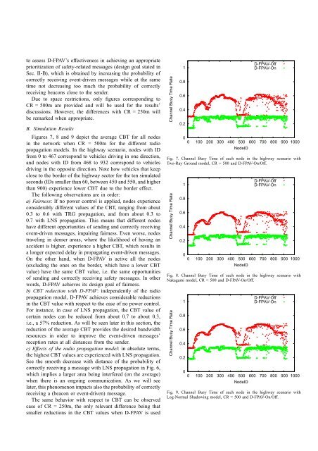
to assess D-FPAV’s effectiveness in achieving an appropriateprioritization of safety-related messages (design goal stated inSec. II-B), which is obtained by increasing the probability ofcorrectly receiving event-driven messages while at the sametime not decreasing too much the probability of correctlyreceiving beacons close to the sender.Due to space restrictions, only figures corresponding toCR = 500m are provided and will be used <strong>for</strong> the results’discussions. However, the differences with CR = 250m willbe remarked when appropriate.B. Simulation ResultsFigures 7, 8 and 9 depict the average CBT <strong>for</strong> all nodesin the network when CR = 500m <strong>for</strong> the different radiopropagation models. In the highway scenario, nodes with IDfrom 0 to 467 correspond to vehicles driving in one direction,and nodes with ID from 468 to 932 correspond to vehiclesdriving in the opposite direction. Note how vehicles that keepclose to the border of the highway sector <strong>for</strong> the ten simulatedseconds (IDs smaller than 60, between 450 and 550, and higherthan 900) experience lower CBT due to the border effect.The following observations are in order:a) <strong>Fair</strong>ness: If no power control is applied, nodes experienceconsiderably different values of the CBT, ranging from about0.3 to 0.6 with TRG propagation, and from about 0.3 to0.7 with LNS propagation. This means that different nodeshave different opportunities of sending and correctly receivingevent-driven messages, impairing fairness. Even worse, nodestraveling in denser areas, where the likelihood of having anaccident is higher, experience a higher CBT, which results ina longer expected delay in propagating event-driven messages.On the other hand, when D-FPAV is active all the nodes(excluding the ones on the border, which have a lower CBTvalue) have the same CBT value, i.e. the same opportunitiesof sending and correctly receiving safety messages. In otherwords, D-FPAV achieves its design goal of fairness.b) CBT reduction with D-FPAV: independently of the radiopropagation model, D-FPAV achieves considerable reductionsin the CBT value with respect to the case of no power control.For instance, in case of LNS propagation, the CBT value ofcertain nodes can be reduced from about 0.7 to about 0.3,i.e., a 57% reduction. As will be seen later in this section, thereduction of the average CBT provides the desired bandwidthresources in order to improve the event-driven messages’reception rates at all distances from the sender.c) Effects of the radio propagation model: in absolute terms,the highest CBT values are experienced with LNS propagation.See the smooth decrease with distance of the probability ofcorrectly receiving a message with LNS propagation in Fig. 6,which implies a larger area being interfered (on the average)when there is an ongoing communication. As we will seelater, this phenomenon impacts also the probability of correctlyreceiving a (beacon or event-driven) message.The same behavior with respect to CBT can be observedcase of CR = 250m, the only relevant difference being thatsmaller reductions in the CBT values when D-FPAV is usedChannel Busy Time Rate10.80.60.40.200 100 200 300 400 500 600 700 800 900 1000NodeIDD-FPAV-OffD-FPAV-OnFig. 7. Channel Busy Time of each node in the highway scenario withTwo-Ray Ground model, CR = 500 and D-FPAV-On/Off.Channel Busy Time Rate10.80.60.40.200 100 200 300 400 500 600 700 800 900 1000NodeIDD-FPAV-OffD-FPAV-OnFig. 8. Channel Busy Time of each node in the highway scenario withNakagami model, CR = 500 and D-FPAV-On/Off.Channel Busy Time Rate10.80.60.40.200 100 200 300 400 500 600 700 800 900 1000NodeIDD-FPAV-OffD-FPAV-OnFig. 9. Channel Busy Time of each node in the highway scenario withLog-Normal Shadowing model, CR = 500 and D-FPAV-On/Off.