InSitu Analysis of Pipeline Metallurgy - dnV

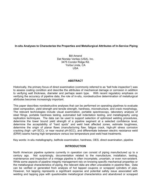
In-situ Analyses to Characterize the Properties and Metallurgical Attributes of In-Service PipingBill AmendDet Norske Veritas (USA), Inc.3475 Condor Ridge Rd.Yorba Linda, CAUSAABSTRACTHistorically, the primary focus of direct examination (commonly referred to as “bell hole inspection”) wasto assess coating condition and describe the attributes of mechanical damage or corrosion in additionto verifying wall thickness, diameter and perhaps seam type. With recent regulatory emphasis onverifying the accuracy of pipeline data, the role of in-situ, nondestructive determination of metallurgicalattributes becomes increasingly important.This paper describes nondestructive analyses that can be performed on operating pipelines to evaluatesteel composition, yield strength and tensile strength, hardness, microstructure, and crack morphology.The relevant technologies include visual examination, portable spectroscopy, laboratory analysis ofsteel filings, portable hardness testing, automated ball indentation testing, and metallography usingreplication techniques. The data can be used to support selection of optimized welding procedures,determine the lower bound yield strength of a pipeline segment at a selected confidence level,determine the acceptability of “hard spots” and weld heat affected zones, estimate toughness,determine the origin of planar flaws (manufacturing flaw, fatigue crack, high-pH stress corrosioncracking (high –pH SCC), or near neutral pH-SCC), and differentiate between electric resistance weld(ERW) seams having high temperature versus low temperature post weld heat treatments.Key words: in-situ metallography, bellhole examination, hardness, OES, direct examination, pipelineINTRODUCTIONNorth American pipeline systems currently in operation can consist of piping manufactured up to acentury ago. Not surprisingly, documentation related to the manufacture, installation, testing,maintenance and inspection of a vintage pipeline is often incomplete, uncertain, or even non-existent.While some aspects of pipeline integrity management rely on knowing specific mechanical properties orthe metallurgical characteristics of piping, the relevant data are often unavailable in pipeline files. Datacan be verified or generated from analysis of hot tapped coupons or scrapped cylinders of pipe.However, hot tapping represents a significant expense and potential safety issue associated withwelding and tapping pipe with questionable metallurgical characteristics and abandoned or scrapped

pipe related to the pipeline segment of interest is not always available. Further, while a single tappedcoupon or pipe cylinder may not be representative of the range of metallurgical characteristics orproperties in a long pipeline segment, obtaining multiple pipe samples for destructive testing can beimpractical. Fortunately, visual examination and interpretation of specific surface featuressupplemented by nondestructive metallurgical analyses can provide a wealth of information tosupplement and/or validate pipeline records.THE VALUE OF VISUAL EXAMINATIONTo a trained inspector, visible features on a pipe surface can reveal details about manufacturingmethods, installation and inspection - details easily overlooked if the focus is merely on characterizingin-service degradation. For example, fillet welded plugs or small patches at the 12:00 position within afew inches of girth welds made in the late 1940s through early 1950s typically indicate that aradiographic isotope was lowered into the pipe to enable single wall exposure radiographic inspectionof the girth weld. 1 The plug or patch was used to seal hole after the inspection was complete.Inspection by radiography has been identified as the leading indicator of girth weld quality.Flush rectangular patches welded across girth welds are indicative of mobile tensile testing units thatwere used on the right of way to spot check girth weld quality before reliable nondestructive testing(NDT) methods were developed. If the test result failed the acceptance criteria the weld would havebeen removed and replaced with a new weld. “Good” welds were patched. While the patch indicatesthat the weld met the specifications for mechanical properties the practice of inserting the welded patchto replace the test specimen was abandoned after it was discovered that the pipelines often leaked atthe patch. 2As another example, specific types of surface textures (“spellerizing”) are uniquely associated with lapseam pipe. The surface pattern was embossed onto the pipe surface by the patterns engraved on therollers that gripped the pipe during processing. The patterns typically occur in two bands with the lapseam located in one of the two bands. Furthermore, since the specific pattern of the spellerizing wasunique to each lap seam pipe manufacturer characterizing the spellerizing pattern can help confirmrecords indicating the pipe manufacturer. 3Surface features are also useful in differentiating furnace butt weld seams from ERW seams. The abilityto differentiate these two types of seams from each other is important mainly because of the lowerseam efficiency factor assigned to butt welded seams by United States federal pipeline safetyregulations (see for example, Reference 4). In addition, butt weld seams are less likely than earlyvintage ERW seams to have very high hardness microstructures in the seam heat affected zone. Thehigh hardness microstructures increase susceptibility to sulfide stress cracking and to brittle fractureinitiation.A few characteristics enable butt seams to be differentiated from ERW seams. First, butt weld seamswere and are only manufactured in pipe no larger than 4.5 inch outside diameter (OD). Second, duringmanufacturing the ERW seam is characterized by flash being expelled to the inside diameter(ID) andoutside diameter of the pipe. It is subsequently machined off nearly flush with the pipe surface. Incomparison, furnace butt welding, or the more modern variant of continuous butt welding, often leavesa perceptible groove along the OD where the seam fusion line is located. Third, the butt weld processoften leaves a characteristic band of scratch marks alongside the seam (Figure 1).Other important surface features are even more subtle than the features on butt weld seam pipe. From1940 to 1951 manufacturers of API Specification 5L pipe were required to stamp the pipe with a markidentifying the manufacturer within 305 mm (12 in.) of the end of the pipe, After the twelfth edition ofAPI 5L painted stencil marks were an acceptable alternative to stamped marks. The stamp marks areshallow and each character is normally only about 6-10 mm (1/4-3/8 in.) across (Figure 2). However,

careful removal of coating and close visual examination of the area near girth welds will sometimesreveal the stamp marks.Girth weld joint designs and weld metal appearance are not frequently characterized during directexamination but they can be significant from the standpoint of assessing likely resistance to large axialstrains such as those associated with ground deformation. Reference 5 describes the evolution ofseveral different types of girth weld joint designs. For example, fillet welded bell+spigot joint designswere largely abandoned in the early 1930s in part because of the relatively low axial strain capacity ofthe fillet welds. In comparison, the bell-bell-chill ring (BBCR) joint design that followed was found tohave much better strain capacity, even when workmanship was imperfect.Oxyacetylene weld deposits are notorious for having workmanship flaws in the weld root and oftenhave a uniquely high and wide cap on the OD surface. While the dimensions of the weld cap areseldom measured in the course of routine bellhole inspection, it has been demonstrated that very widecaps (width at least five time the wall thickness) having a height greater than 50% of the wall thicknessreduce the applied stress intensity factor by a minimum of 25%. Smaller caps have smaller influencewith the effect being related to cap height to width ratio and dimensions relative to the pipe wallthickness. As a result, the strain capacity of the welds can be somewhat larger than what is expectedbased on conventional fracture mechanics evaluations that disregard the cap effects. 6 Therefore,recording the dimensions of weld caps can support fitness for service assessments of welds.One typically overlooked feature of early girth welds is the consistency of the weld metal ripple patternthat indicates the direction of weld progression. Early pipeline construction techniques included thepractice of making several girth welds above ground while pipe was rolled underneath the welding arcor torch. Segments of welded pipe were then placed into the ditch and welded together in the morechallenging fixed position. Sometimes different welding processes were used for the two different typesof welds. The rolled position and fixed position welds result in different weld ripple patterns that areeasily distinguishable from each other. In more modern pipe similar weld to weld variations inworkmanship and properties exist when pipe segments are made using pipe that is “double jointed”,typically using submerged arc welding, at the mill prior to being delivered to the construction site. As aresult of the two different welding positions and/or use of different welding processes for different girthwelds the long pipeline segments can have two (or more) distinctly different populations of girth welds.Each weld population can have different workmanship quality and mechanical properties that occurrepeated sequences. Identifying the presence of multiple populations of girth welds can influenceintegrity assessment sampling plans and assessment methodologies.Sometimes visual examination must be supplemented with NDT to differentiate among seam types.For example, single side submerged arc welded (SSAW) and double sided submerged arc welded(DSAW or SAW-L) seams look the same from the OD surface. Only the ID appearance is different.Normally, the differences are apparent in radiographic inspection.In another example, two separate types of seams are commonly mischaracterized as a product of anearly submerged arc welding process when in fact they are both unique types of seams manufacturedfrom about 1928 to 1932 by A.O. Smith Corporation. (1) The external appearance of both types ofseams is the same as a result of both types using a relatively broad, flat cap pass of metal deposited byshielded metal arc welding (Figure 3). In both types of seams weld metal solidification cracks are oftenfound in the cap pass. Until 1930 the seam consisted only of multiple passes of weld metal depositedby shielded metal arc welding process. Incomplete penetration and lack of fusion in the root region iscommonly observed. By 1930 the root portion of the seam was first formed by the flash weld processand the cap pass was used only for additional reinforcement. As a result, the OD of the pipe isindistinguishable from the earlier vintage pipe while the ID looks like a conventional flash welded seam.1 Trade name.

While the mechanical properties of the cap can be similar in both types of seam the properties beneaththe cap can be quite different.Chemical CompositionChemical analysis in the field is used by a variety of industries to verify the composition of incomingcorrosion resistant, heat resistant, or high strength alloys. However, in the pipeline industry, chemicalanalysis is most frequently performed on in-service pipelines to determine carbon equivalent of thesteel to support selection of optimized welding procedures. Therefore, for pipeline applications thechemical analysis methods must be capable of accurately measuring the elements that are included inthe applicable carbon equivalent equations. The most frequently used equations are the CE IIW andPcm equations shown below in Equations 1 and 2.:CE IIW : %C + %Mn/6 + (%Cr+%Mo+%V)/5 + (%Ni+%Cu)/15 (1)Pcm: %C + (%Cr+%Cu+%Cr)/20 + %Ni/60 + %Mo/15 +%V/10 + 5x%B (2)However, of the available field portable PMI (positive metal identification) techniques, only the opticalemission spectrography (OES) method is capable of measuring carbon (atomic number 6) (Figure 4).The x-ray fluorescence (XRF) method will not typically detect and measure elements lighter than atomicnumber 12 (magnesium). Even some portable OES devices are not capable of measuring carbon withsufficient accuracy. Those that use an argon flushed sensor normally provide the best determination oflight elements.In our experience, preparation of steel pipe surfaces for PMI includes first removing at least 0.25 mm(0.01 in.) of the pipe surface to minimize or eliminate the influence of the decarburization that is oftenpresent on the ID and OD surfaces (Figures 5 and 6). Inadvertent inclusion of the decarburized surfacein the analysis results in measurement of an anomalously low carbon content. In view of the ease ofsurface preparation and performance of the measurements, three measurements are normally made,including at least one measurement on either side of the longitudinal seam (for example, about 50-75mm (2-3 in.) from the seam). After the completing the measurements, the metallurgical effects of the“burned” spot caused by the arcing can easily be removed by using a powered sanding disc.Metallographic cross sections through typical spectrographic burn marks show that the related heataffected zone is only about 30 microns (1.2 mils) deep (Figure 7).Note that the results of field portable spectrographs are sensitive to maintenance and calibration. Aninstrument can appear to be functioning properly but produce results that are significantly different fromthose obtained from standard laboratory chemical analysis methods. Sometimes the results for onlyone or a few elements are inaccurate and technicians are not always adequately trained to recognizethe questionable results. Verification of proper instrument maintenance and on-site verification ofcalibration is important.The alternative method of determining the chemical composition of the steel involves removing steelfilings from the steel surface and then analyzing the filings using traditional chemical analysis methodsin a laboratory (Figure 8). As in the case of the PMI measurements, filings should not be collected untilat least 0.25 mm (0.01 in.) of the pipe surface have been removed to minimize the effect ofdecarburization. The procedure for collecting the filings is detailed in Attachment A). While theprocedure references a specific suggested volume of filings, the required amount of filings should beverified with the specific laboratory that is performing the analysis.While removing steel from the pipe surface would seem to be destructive in nature, it is rarelynecessary to remove a total of more than about 0.4-0.5 mm (16-20 mils) of the pipe surface (includingthe initial removal of 0.25 mm (10 mils) to minimize the effects of decarburization) from an area about 6inches in diameter to obtain enough material for analysis. A thickness reduction of 0.5 mm (20 mils)

from a pipe having a nominal original wall thickness of 4.78 mm (0.188) inches represents a localizedthickness reduction of only 10.6% of the wall thickness. The example below illustrates the effect of themetal removal on the integrity of a hypothetical pipeline.Pipe specification: API 5L X42O.D.: 219 mm (8.625 in.)Wall thickness: 4.78 mm (0.188 in.)Diameter of metal loss: 152 mm (6 in.)Depth of metal removal: 0.5 mm (0.02 in.)Calculated failure pressure using the effective area method of RSTRENG: 114% SMYSFor the hypothetical example of removing filings from a thin wall pipe, no repair would be required otherthan recoating the exposed steel since the failure pressure exceeds the SMYS. The same metal losson thicker wall pipe would be even less significant.The surface area and depth of metal removal required to collect the required mass of steel filings foranalysis can be approximated from Equation 3.M req / (16.39 cm 3 /in 3 x 7.86 gm/cm 3 ) = L x W x d (3)Where: M req = milligrams of filings required for analysisL = length of area from which filings are removed (in.)W = Width of area from which filings are removed (in.)d = depth of removal (after removal of 10 mils) (mils)Hardness TestingHardness testing on pipelines can be performed for a variety of purposes, including:Evaluating the acceptability of “hard spots” on pipe surfacesChecking weld heat affected zone hardnessChecking ERW seams and other seams for evidence of effective postweld heat treatmentEstimating tensile strength and lower bound yield strengthHard heat affected zones can be subject to cracking from exposure to fluids containing H 2 S (i.e., “sourservice”) or from the combined presence of sufficient amounts of stress, hydrogen from welding, andhard microstructures (i.e., “hydrogen cracking” or “underbead cracking”).Several types of field-portable hardness testers are available for determining the acceptability of hardspots, weld heat affected zones, or for determining the lower bound expected yield strength. However,each hardness tester has its own strengths and limitations. For example, results from some hardnesstest methods are significantly influenced by technique, material thickness, surface curvature andsurface preparation and may even be affected by residual magnetism, vibration, or temperature. 7One of the most obvious differences among different hardness test methods pertains to the volume ofthe metal that is sampled by the indentation. The indentations produced by a telebrineller have aspherical cap profile that may be a few millimeters across, thus making them suitable for measuring thegeneral hardness of an area, but unsuitable for measuring the maximum hardness of a weld heataffected zone. In contrast, the pyramid shaped indentations associated with the ultrasonic compact(UCI) method may be barely visible to the unaided eye (Figures 9 and 10).

Considerations in the selection of a specific test method for use in the field include: Test material thickness limits and need for thickness-related correction factors. This isparticularly applicable to the Leeb (ball rebound) hardness test method in which correctionfactors for thickness are recommended for substrates less than about 22 mm (0.875 in.) thick,and correction factors can be quite large for wall thicknesses less than about 8 mm (0.3 in.). Influence of residual magnetic fields, particularly for methods that rely on measurement of ballrebound velocity. Ambient temperature limitations, especially for methods that use electronic equipmentEffects of pipeline vibrationSensitivity to technician technique. Results from handheld probes, especially UCI hardness testindentors can be sensitive to impingement angle (Figure 3).The need for more precise surface preparation increases as indentation size decreases. For both theLeeb ball rebound hardness test method and the UCI hardness test method ASME (2) CRTD Vol. 91recommends a surface finish no coarser than 180 grit, obtained after use of a series of abrasivesanding discs having successively finer abrasive grit size. 7 Hardness test results most representativeof the “bulk” hardness of the pipe wall are obtained after removal of at least 0.01 inches of the pipesurface so that the results are not influenced by surface decarburization. (Figure 4).ASME CRTD Vol. 91 contains extensive information about hardness tester selection and use forpipeline applications. However, the majority of the report and an accompanying Checklist fortechnicians 8 describes the process for using field hardness testing on randomly selected pipe joints toestimate the lower bound yield strength of a pipeline segment. The relationship of base metal hardnessto ultimate tensile strength has been long recognized, but the relationship of hardness to yield strengthhas only been more recently studied. Two ASME CRTDs have been issued describing the correlationbetween Rockwell B hardness and predictions of lower bound yield strength for pipes meeting adefined set of boundary conditions related to age, size, and strength. 7,9] The correlations are applicableto determining the lower bound yield strength of individual tested pipeline joints and, when combinedwith a defined statistical analysis procedure and data from multiple pipe joints, the correlation can beused to calculate the lower bound yield strength of a pipeline segment at a selected confidence level.Converting measured hardness into estimates of yield strength is based on empirical data and requiresstrict adherence to boundary conditions (pipe size, age, etc.) to ensure that the established relationshipof hardness to strength is applicable. 9 Those boundary conditions include: Pipe diameter no smaller than 114 mm (4.5 in.) OD D/t no smaller than 20 359 mpa (52 ksi) and lower specified minimum yield strength (SMYS) Pipe manufactured before 1980In addition, when determining the lower bound yield strength for all pipe joints within a pipeline segmentbased on random sampling of pipe joints, all of the joints within the segment must be from a single pipepopulation having characteristics that meet the boundary conditions described above and also have noevidence of being from different pipe lots. Reference 7 defines a pipe population or lot as a set of pipejoints having the same size, age, seam type and source.(2) ASME International, Three Park Ave., New York, NY 10016-5990.

In-situ MetallographyIn-situ metallography is a process of performing a modified version of a laboratory metallographicsample preparation and examination under field conditions. Proper polishing and etching techniquesand interpretation of replicated surfaces is a key to success. One key difference between laboratoryand in-situ metallography is that laboratory procedures usually involve preparation and examination ofcross sectional views of a pipe wall, whereas in the field, the preparation and examination is performedon the plane approximately parallel to and just slightly below the outside surface of the pipe. As aresult, through-thickness variations in the microstructure or crack morphology are not apparent in in-situmetallographic results. For example, stress corrosion cracking can initiate at the base of a mill flaw thatcauses a local stress concentration. However, the transition from mill flaw to SCC may be undetectedby metallographic examination of a prepared area that represents only a single plane parallel to andjust slightly below the pipe surface.The pipe surface is prepared by wet grinding small areas (i.e., a few square inches) of the pipe surfacewith a series of successively finer adhesive-backed abrasive discs mounted in a drill or similar powertool. The grinding typically finishes with 600 grit abrasive. Following the use of the abrasive discs, thesurface is polished with one or more diamond abrasive pastes, typically ending with a particle size nocoarser than about 6 micron. A final polish is obtained using either finer diamond abrasives or aluminaslurry. In all polishing stages the abrasive is normally applied to a small cloth disc that is once againmounted on and powered by a drill or similar power tool. During the grinding and polishing stages, caremust be taken to completely eliminate the scratches caused by the previous abrasive beforetransitioning to the next finer abrasive. Remnants of inadvertent cold working (superficial smearing) ofthe surface can be further minimized by etching the surface with nital or another etchant, followed byrepolishing with the finest abrasive, and then re-etching. Alternatively, surfaces may be electropolishedand then etched, although electropolishing can sometimes have a detrimental effect on some types ofinclusions.After the final etching step, the surface can be viewed directly with a field-portable microscope, or thetopography of the etched surface can be replicated for viewing later at a laboratory (Figures 11 through13). Replication can be performed by a few different methods. Acetate film tape can be softened withacetone and then pressed against the etched surface and then peeled off when it rehardens after a fewminutes. Alternatively, a castable resin (example, Struers “RepliSet” (3) system of fast curing two-partsilicone rubber) or proprietary replica foil consisting of reflecting plastic film with self-adhesive backingcan be used to replicate the etched topography of the prepared surface. The tape or casting can betransported to a laboratory and be viewed directly with a metallurgical microscope or can be coatedwith vaporized carbon and viewed with a scanning electron microscope. Resolution to 0.1 microns isachievable. Details of in-stu metallographic procedures are described in Reference 10.The Question of ToughnessToughness is a key input when determining the failure stress of planar flaws and in predicting leakversus rupture behavior. While toughness is normally measured in various types of destructive fracturetoughness tests or Charpy impact tests, efforts to estimate toughness via in-situ nondestructivemeasurements continues. Toughness is known to have qualitative relationships to pipe characteristicsthat can be measured nondestructively, including chemical composition, microstructure, and grain size.Quantitative relationships between composition and grain size in ferrite-pearlite steels have beenpublished, for example, Equation 4. 11(3) Trade name.TT = -19 +44(Si) + 7000(Nf 0.5 ) + 2.2(P) – 11.5 (d .-0.5 ) . (4)

Where TT = Charpy transition temperature (°C)Si = silicon (%)Nf = free nitrogen content (%)P = phosphorous (%)d = ferrite grain size (mm)DNV (4) staff have observed that the relationship of toughness data to pipeline composition data derivedfrom OES analysis can be relatively consistent for pipes within a single population of pipe joints.However, for other populations of pipe different relationships of toughness to composition appear to fitbetter.Methods based on the automated ball indentation (ABI) test technique have been described andevaluated by various researchers and service providers. 12 The ABI method is nondestructive andcapable of measuring data regarding true stress-true strain characteristics from which tensile propertiescan be derived. More recent work has been aimed at demonstrating the ability to derive fracturetoughness properties as well. We have found no North American or European standard that covers theuse of ABI methods for measurement of tensile or fracture toughness properties.The power generation industry has used small punch test (SPT) specimens to estimate tensile andfracture toughness properties, but the procedures are not yet standardized by ASTM (5) or standardsorganizations in the European Union. The specimens encompass a range of sizes and shapes, agenerally ranging in size from 3 to 10 mm (0.12 to 0.40 in.) in diameter and between 0.1 to 0.75 mm(0.004 to 0.03 in.) thick. 13 Although the specimen thickness is small, a considerable amount of the wallthickness of a typical transmission pipeline could be affected by the machining operation that removesthe required material from which the specimen is made.(4)Det Norske Veritas (USA), Inc., 5777 Frantz Rd. Dublin, OH 43017.(5) ASTM International, 100 Barr Harbor Dr., West Conshohocken, PA 19428-2959.

ScratchesFigure 3:Typical appearance of the outsidesurface of seams made by A.O. Smith fromabout 1928 through about 1932. (Scale ininches)GrooveFigure 1: Surface of continuous butt weldseam pipe showing characteristic grooveand band of subtle scratches. (Scale ininches)Figure 4:Typical in-field use of portable OESchemical analysis equipment.1 in. (25mm)Figure 2: Stamp marks near the end of aseamless pipe identifying the manufactureras Youngstown Steel & Tube Co.

Figure 5: Areas on either side of a girthweld on 16 in. pipe prepared for hardnesstesting and chemical analysis. Coating hasbeen stripped and the steel cleaned to shinymetal and at least 0.01 in. has been removedfrom the surface. Each area isapproximately six to eight inches long.Figure 7: Metallographic cross sectionthrough OES chemical analysis burn markon high carbon equivalent steel. Arrowindicates the approximate extent of the heataffected zoneFigure 6: Metallographic cross sectionshowing alteration of the near-surfacemicrostructure resulting fromdecarburization of the steel duringprocessing at high temperatures.Figure 8: An example of a set-up for thecollection of steel filings used for chemicalanalysis

Figure 10: Magnified view of a normal UCIhardness indentation (at left) and examplesof poor test technique (at right)Figure 9: Pipe surface having small “puddleweld” used to repair external corrosion (attop), and the same area after polishing andetching to show the weld heat affected zoneand being hardness testing using the UCItest method (bottom). Two of the manyhardness indentations are circled.Figure 11: Image of a metallographic replicashowing significant microstructuraldifferences on either side of a linearindication revealed by magnetic particleinspection. The microstructural variationsindicate that the indication is a mill flaw,rather than any form of in-service cracking

Figure 12: A higher magnification exampleof microstructural variations typical of millflaws.Figure 13: Oxide-filled intergranular crackstypical of microstructural replicas of highpHSCC. Note that the microstructure isconsistent on both sides of the cracking.CONCLUSIONSDirect examination offers the opportunity for learning much about the metallurgical characteristics of anexposed pipeline in addition to characterizing in-service damage and coating degradation. Carefulvisual examination by technicians trained to identify and interpret specific features combined with oneor more non-destructive analysis techniques can help pipeline operators validate uncertain pipelinerecords and provide important data in the pipeline integrity management process.REFERENCES1. E. Sterrett, “Pipelines Across the Desert”, Welding Engineer Vol 34, No. 4, April, 19492. Anon., “Report of the Natural Gas Transmission Pipe Lines Committee”, Proceedings of the Thirty-Sixth Annual Convention of the Pacific Coast Gas Association, Del Monte, California, September10-13, 19293. J.F. Kiefner, E.B. Clark, History of Line Pipe Manufacturing in North America, CRTD Vol. 43, ASME19964. Anon. Electronic Code of Federal Regulations, Title 49 Part 192 “Transportation of Natural andOther Gas by Pipeline: Minimum Federal Safety Standards”, § 192.113 Longitudinal joint factor (E)for steel pipe http://ecfr.gpoaccess.gov/cgi/t/text/textidx?c=ecfr&tpl=/ecfrbrowse/Title49/49cfr192_main_02.tplSeptember 27, 20125. W. E. Amend, “Vintage Girth Weld Assessment – Comprehensive Study”, PRCI contract PR-355-094502 final report, March 5, 20106. K. Koppenhoefer “Factors Influencing Girth Weld Reliability in Older Pipelines”, PRCI contract PR-185-9830, final report, October 31, 20037. E.B Clark, W.E. Amend, “Applications Guide for Determining the Yield Strength of In-Service Pipeby Hardness Evaluation, Final Report”, CRTD -Vol. 91, (City, State: ASME) 20098. B. Amend, “Using Hardness to Estimate Pipe Yield Strength; Field Application of ASME CRTD -Vol. 91”, Proceedings of the 2012 9th International Pipeline Conference IPC2012-90262 (City,State: ASME)9. D.A. Burgoon, O.C. Chang, et.al, “Final Report on Determining the Yield Strength of In-servicePipe” CRTD -Vol. 57, (City, State: ASME), December 199910. ASTM E 1351 “Standard Practice for Production and Evaluation of Field Metallographic Replicas”.(West Conshohocken, PA: ASTM)

11. B.L. Bramfitt, “Structure/Property Relationships in Irons and Steels”, Metals Handbook DeskEdition, Second Edition, J.R. Davis, editor, 199812. K. Sharma, P.K. Singh, et al., “Application of Automated Ball Indentation for Property Measurementof Degraded Zr2.5Nb” Journal of Minerals & Materials Characterization & Engineering, Vol. 10,No.7, pp.661-669, 201113. J.R. Foulds, M. Wu, S. Srivastav, and C.W. Jewett, “Fracture and Tensile Properties of ASTMCross Comparison Exercise A 533B Steel by Small Punch Testing”, Small Speciman Testtechniques, ASTM STP 1329, W.R. Corwin, S.T. Rosinski, E. van Walle editiors, ASTM, 1998ATTACHMENT 1COLLECTION OF STEEL FILINGS FOR CHEMICAL ANALYSISMATERIALS / TOOLS NEEDEDSample containerCarbide burrElectric or pnuematic drill with 3/8 inch chuckTools to remove pipe coatingGrinder or drill equipped with coarse to medium grit sanding disks (example: 40-100 grit)File folder or similar stiff paper or cardboard approx. 12x 18 inches or larger (when opened flat)Duct tape or similarSafety glasses / gogglesMagnetPlastic wrap or plastic bagPROCEDURE1. Strip coating from pipe in area approximately 1 ft x 1 ft located at approximately the 1:00 to 3:00position2. Use sanding disks or grinder to remove pipe coating residue and any other contamination from areaapprox. 9 x 9 inches. Metal should be shiny with no specks of dirt, rust, oxide scale, paint, or otherforeign material present. For best results remove about 0.01 inches of thickness before starting thecollection of filings3. Open the file folder and tape one 12-inch side of file folder to bottom of cleaned area on the pipe.Run the tape along the entire edge of the folder. The open file folder should now be hanging downfrom the pipe.4. Fold the file folder in half to form a vee-shaped trough into which steel filings can fall5. Use two pieces of tape (one on each side) to bridge across the two sides of the vee so that whenyou let go of the file folder the “vee” shape still remains. The “loose” or unattached side of the filefolder will stand out from the pipe at about a 30-45 degree angle6. Hold the drill against the cleaned pipe so that the direction of burr rotation will push the steelshavings into the bottom of the vee-shaped file folder trough.7. Use a drill speed which allows you to control the direction and distance that the steel shavings arethrown. A burr RPM that is too fast will cause the chips to be flung past the collection trough.8. Check the burr occasionally for evidence of chipped cutting edges. If the burr is chipped thendiscard the filings, mount a new burr, and continue collecting filings9. Peel the tape off the pipe while being careful not to spill the filings10. Dump the filings into the sample container if no evidence of chipping is seen on the burr teeth.11. Reattach the file folder as in step 3-5 and continue to collect filings.

12. Collect enough shavings to form a volume about as large as a stack of 3 nickels or more13. Before submitting the filings for analysis, dump the filings on paper and drag a magnet wrapped inplastic wrap through the filings to collect the steel and leave any dirt, paint chips, rust, behind. Pullthe magnet out of the plastic wrap. The filings will fall away into a sample vial. Repeat this cleaningprocess until no evidence of nonmagnetic materials are left behind after dragging the magnetthrough the filings and no foreign material is visible in the filings.