Decoherence and the Bloch equations

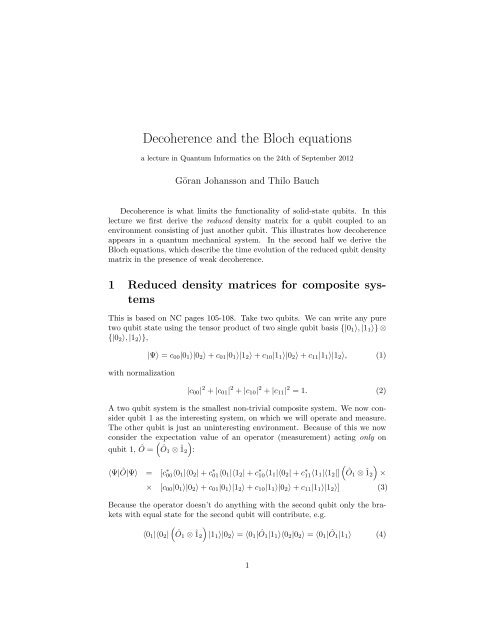
Decoherence and the Bloch equationsa lecture in Quantum Informatics on the 24th of September 2012Göran Johansson and Thilo BauchDecoherence is what limits the functionality of solid-state qubits. In thislecture we first derive the reduced density matrix for a qubit coupled to anenvironment consisting of just another qubit. This illustrates how decoherenceappears in a quantum mechanical system. In the second half we derive theBloch equations, which describe the time evolution of the reduced qubit densitymatrix in the presence of weak decoherence.1 Reduced density matrices for composite systemsThis is based on NC pages 105-108. Take two qubits. We can write any puretwo qubit state using the tensor product of two single qubit basis {|0 1 〉, |1 1 〉} ⊗{|0 2 〉, |1 2 〉},with normalization|Ψ〉 = c 00 |0 1 〉|0 2 〉 + c 01 |0 1 〉|1 2 〉 + c 10 |1 1 〉|0 2 〉 + c 11 |1 1 〉|1 2 〉, (1)|c 00 | 2 + |c 01 | 2 + |c 10 | 2 + |c 11 | 2 = 1. (2)A two qubit system is the smallest non-trivial composite system. We now considerqubit 1 as the interesting system, on which we will operate and measure.The other qubit is just an uninteresting environment. Because of this we nowconsider the expectation ) value of an operator (measurement) acting only onqubit 1, Ô =(Ô1 ⊗ ˆ1 2 :)〈Ψ|Ô|Ψ〉 = [c∗ 00〈0 1 |〈0 2 | + c ∗ 01〈0 1 |〈1 2 | + c ∗ 10〈1 1 |〈0 2 | + c ∗ 11〈1 1 |〈1 2 |](Ô1 ⊗ ˆ1 2 ×× [c 00 |0 1 〉|0 2 〉 + c 01 |0 1 〉|1 2 〉 + c 10 |1 1 〉|0 2 〉 + c 11 |1 1 〉|1 2 〉] (3)Because the operator doesn’t do anything with the second qubit only the braketswith equal state for the second qubit will contribute, e.g.)〈0 1 |〈0 2 |(Ô1 ⊗ ˆ1 2 |1 1 〉|0 2 〉 = 〈0 1 |Ô1|1 1 〉〈0 2 |0 2 〉 = 〈0 1 |Ô1|1 1 〉 (4)1

while)〈0 1 |〈1 2 |(Ô1 ⊗ ˆ1 2 |1 1 〉|0 2 〉 = 〈0 1 |Ô1|1 1 〉〈1 2 |0 2 〉 = 0. (5)Of the original 16 terms we are left with eight〈Ψ|Ô|Ψ〉 = [c∗ 00〈0 1 | + c ∗ 10〈1 1 |] Ô1 [c 00 |0 1 〉 + c 10 |1 1 〉] +which we should regroup+ [c ∗ 11〈1 1 | + c ∗ 01〈0 1 |] Ô1 [c 11 |1 1 〉 + c 01 |0 1 〉] , (6)〈Ψ|Ô|Ψ〉 = 〈0 1|Ô1|0 1 〉 [ |c 00 | 2 + |c 01 | 2] + 〈0 1 |Ô1|1 1 〉 [c ∗ 00c 10 + c ∗ 01c 11 ] ++ 〈1 1 |Ô1|0 1 〉 [c ∗ 10c 00 + c ∗ 11c 01 ] + 〈1 1 |Ô1|1 1 〉 [ |c 10 | 2 + |c 11 | 2] . (7)We can now construct a reduced density matrix, for the first qubit only[ ]|c00 |ρ 1 =2 + |c 01 | 2 c ∗ 10c 00 + c ∗ 11c 01c ∗ 00c 10 + c ∗ 01c 11 |c 10 | 2 + |c 11 | 2 , (8)which reproduce 〈Ψ|Ô|Ψ〉 = T r(ρ 1O 1 ). We can check that T r(ρ) = 1 and thatit is Hermitian, so it is a valid density matrix. The reduced density matrix forqubit 1, ˆρ 1 , can be also obtained from the pure two qubit density matrix |Ψ〉〈Ψ|,with |Ψ〉 given by Eq. 1, by tracing out the second qubitˆρ 1 = T r 2 (|Ψ〉〈Ψ|) =1∑〈j 2 | [|Ψ〉〈Ψ|] |j 2 〉 =j=0= 〈0 2 |Ψ〉〈Ψ|0 2 〉 + 〈1 2 |Ψ〉〈Ψ|1 2 〉 == |0 1 〉〈0 1 | [ |c 00 | 2 + |c 01 | 2] + |0 1 〉〈1 1 | [c ∗ 10c 00 + c ∗ 11c 01 ] ++ |1 1 〉〈0 1 | [c ∗ 00c 10 + c ∗ 01c 11 ] + |1 1 〉〈1 1 | [ |c 10 | 2 + |c 11 | 2] . (9)For a product state |Ψ〉 = |Ψ 1 〉|Ψ 2 〉 = [ c 1 0|0 1 〉 + c 1 1|1 1 〉 ] [ c 2 0|0 2 〉 + c 2 1|1 2 〉 ] we havec 00 = c 1 0c 2 0, c 01 = c 1 0c 2 1, c 10 = c 1 1c 2 0 and c 11 = c 1 1c 2 1. Putting this into Eq. 8,and using the normalization |c 2 0| 2 + |c 2 1| 2 = 1, gives the ordinary pure statedensity matrix for qubit 1, ρ 1 = |Ψ 1 〉〈Ψ 1 |. Instead choosing a Bell state |Ψ〉 =(|0 1 〉|0 2 〉 + |1 1 〉|1 2 〉) / √ 2, i.e. c 00 = c 11 = 1/ √ 2 and c 01 = c 10 = 0 gives[ 1]ρ 1 = 201 , (10)02which we recognize as density matrix of a mixed state with fifty/fifty spin upand down in an arbitrary direction, which maps onto the origin of the Blochsphere r = (0, 0, 0). So even if the two qubits together are in a pure state, qubitnumber 1 will behave like a mixed state.2

2 A two-level atom coupled to a thermal bathof harmonic oscillatorsConsider the Hamiltonian of a two-level atom weakly coupled to a thermal bathof harmonic oscillatorsH = −¯hω 02 σ z + ∑ kH c = (η z σ z + η x σ x ) ∑ k¯hω k â † kâk + H c ,g k(â k + â † k), (11)where the coupling is weak compared to the atom frequency |H c | ≪ ¯hω 0 . Thecoupling constants η z and η z determine how much the bath couples to the zand x directions of the atom. The bath of harmonic oscillators can e.g. bethe electromagnetic field in a transmission line or more abstractly some bosonicdegrees of freedom we didn’t manage to decouple completely.We then consider the combined atom-bath density matrix in the interactionpicture,ρ rf (t) = R(t)ρ(t)R(t) †using the operator (see e.g. section 4 in the Rabi lecture notes)R(t) = e −i ω 02 tσ ze i ∑ k ω kâ † kâkt ,the quick coherent dynamics is rotated away and we’ll get a differential equationfor the bath induced dynamics onlyi¯h ˙ρ rf (t) = [H c,rf (t), ρ rf (t)] , (12)where the coupling hamiltonian in the interaction picture isH c,rf (t) = R(t)H c R(t) †= ( η z σ z + η x[σ− e −iω0t + σ + e iω0t]) ∑kg k(â k e −iω kt + â † k eiω kt )≡ A(t)B(t), (13)where A(t) is an operator operating on the atom only and B(t) is a bath operator.In order to perform a perturbation expansion to the second order in thenoise we first rewrite the Liouville equation on a differential-integral form[i¯h ˙ρ rf (t) = H c,rf (t), ρ rf (0) + 1 ∫ t]dt ′ [H c,rf (t ′ ), ρ rf (t ′ )] . (14)i¯hThe idea is now to trace out the bath from this equation and arrive at adifferential equation for the atom density matrix only. We then assume that thebath density matrix is thermal with temperature T , i.e.( )T r B â † kâk ′ = δ k,k ′n k ,03

wheren k =1exp (¯hω k /k B T ) − 1 ,is the average number of photons in the oscillator with frequency ω k accordingto the Bose distribution. Furthermore, we assume that the bath density matrixdoes not change during the system dynamics, mainly because the bath is largeand the atom is small. Also assuming that the atom and bath are in a productstate before the coupling is switched on at t = 0, there will be no contributionto the dynamics from the first order in H c,rf sinceleaving the second order contributionT r B {H c,rf (t)} = 0,˙ρ rf (t) = − 1 ∫ t¯h 2 dt ′ (H c,rf (t)H c,rf (t ′ )ρ rf (t ′ ) + ρ rf (t ′ )H c,rf (t ′ )H c,rf (t)−0− H c,rf (t)ρ rf (t ′ )H c,rf (t ′ ) − H c,rf (t ′ )ρ rf (t ′ )H c,rf (t)]), (15)which we then trace over the bath, to arrive at an equation of motion for the(reduced) atom density matrix only ρ a . The bath operators then appear in thefollowing bath correlation functionf B (t − t ′ ) = T r B {B(t)B(t ′ )} = ∑ [gk2 (1 + n k )e −iω k(t−t ′) ] + n k e iω k(t−t ′ ),kand for the term with the opposite time-orderning we use f B (t ′ − t),˙ρ a (t) = − 1 ∫ t¯h 2 dt ′ (f B (t − t ′ )A(t)A(t ′ )ρ a (t ′ ) + f B (t ′ − t)ρ a (t ′ )A(t ′ )A(t)−0− f B (t ′ − t)A(t)ρ a (t ′ )A(t ′ ) − f B (t − t ′ )A(t ′ )ρ a (t ′ )A(t)) . (16)The bath correlation function thus depends on the couplings g k and temperature.Typically the function is close to a delta-function in time, and its widthis given by the inverse bandwidth of the coupling to the bath.2.1 Purely longitudinal noiseFor η x = 0 and η z = 1, the bath couples only to the time-independent A(t) = σ z ,and we have purely longitudinal noise, i.e. directed along the axis of coherentprecession. This will make the precession velocity uncertain and dephase thequbit. For the equation of motion for the reduced density matrix we have˙ρ a (t) = − 1 ∫ t¯h 2 dt ′ (f B (t − t ′ )ρ a (t ′ ) + f B (t ′ − t)ρ a (t ′ )−0− f B (t ′ − t)σ z ρ a (t ′ )σ z − f B (t − t ′ )σ z ρ a (t ′ )σ z )= − 1 ∫ t¯h 2 dt ′ (f B (t − t ′ ) + f B (t ′ − t)) (ρ a (t ′ ) − σ z ρ a (t ′ )σ z ) . (17)04

Now, using that the bath correlation function f B (t) is close to a delta-function,we can replace t ′ with t in the argument of the density matrix on the right handside, and also extend the region of integration to infinity, to arrive at˙ρ a (t) = − 1∫ t¯h 2 (ρ a(t) − σ z ρ a (t)σ z ) dt ′ (f B (t − t ′ ) + f B (t ′ − t)) , (18)−∞which is a ordinary differential equation. From the matrix structure,[]0 ρρ(t) − σ z ρ(t)σ z = 201 (t)ρ 10 (t) 0we see that this equation describes exponential decrease of the off-diagonal elementsof the density matrix ρ 01 (t) = ρ 01 (0)e −Γ∗ 2 t , where the pure dephasingrate is given byΓ ∗ 2 = 2¯h 2 ∫ t−∞= 2¯h 2 ∫ ∞dt ′ (f B (t − t ′ ) + f B (t ′ − t)) =−∞dτ ∑ kg 2 k(1 + 2n k )e −iω kτ ≡ 2S B (0), (19)whereS B (ω) = 1¯h 2 ∫ ∞−∞dτe −iωτ ∑ kgk2 [(1 + nk )e iωkτ + n k e −iω kτ ]is (single-sided) noise spectral density of the bath, which is nothing but theFourier transform of the bath correlation function.Remembering the mapping of the density matrix in the Bloch sphereρ = 1 + r xσ x + r y σ y + r z σ z2= 1 2[ ]1 + rz r x − ir y, (20)r x + ir y 1 − r zwe realize that the disappearance of the off-diagonal elements implies that r xand r y approaches zero, i.e. the state approaches its projection on the z-axis.Thus we get a mixed state. The phase of the atom becomes entangled with thestate of the bath, and tracing out the bath we get a mixed state of the atom.2.2 Purely transversal noiseFor η z = 0 and η x = 1we have purely transversal noise, i.e. directed perpendicularto the axis of coherent precession. For simplicity we consider couplingonly to σ x . Again, using the short correlation time of the bath we arrive at thedynamics of the atom density matrix[]Γ˙ρ a (t) = ↓ ρ 11 (t) − Γ ↑ ρ 00 (t) − Γ ↑+Γ ↓2ρ 01 (t)− Γ ↑+Γ ↓2ρ 10 (t) Γ ↑ ρ a 00(t) − Γ ↓ ρ a , (21)11(t)5

where the relaxation rateand excitation rateΓ ↓ = S B (ω 0 ) ≈ 2πg 2 ω 0(1 + n ω0 )Γ ↑ = S B (−ω 0 ) ≈ 2πg 2 ω 0n ω0are given by the bath noise spectral density at the frequency of the atom transition.We see that the ration between the relaxation and excitation is given bythe temperature of the bath onlyΓ ↑Γ ↓= n ω 01 + n ω0= e −¯hω0/k BT .Both off-diagonal elements also decay exponentially due to transverse noise withthe rate (Γ ↑ + Γ ↓ )/2.3 Bloch equationsThe Bloch equations were introduced in 1946 in the context of nuclear magneticresonance (NMR). They describe the motion of a spin-1/2 on the Bloch sphere(r(t)) under the influence of control fields B(t) and dissipation described byphenomenological timescales for relaxation/mixing T 1 and dephasing T 2 :ṙ = −B × r − 1 (rz − r 0 ) 1z ẑ − (r xˆx + r y ŷ) , (22)T 1 T 2where r 0 z is the steady state projection on the z-axis. In the previous section wederived:Γ ↑Γ ↑ = S B (−ω 0 ), Γ ↓ = S B (ω 0 ), = e −¯hω0/k BTΓ ↓1= Γ ↓ + Γ ↑ , rz 0 = Γ ↓ − Γ ↑= tanh ¯hω 0T 1 Γ ↓ + Γ ↑ 2k B T ,11T2∗ = 2S B (0), = 1T 2 T2∗ + 1 , (23)2T 1where we assumed the noise arising from a source at temperature T .4 Driven Bloch equations - describing a driventransmon in a transmission lineWe start from the hamiltonian of a transmon with frequency ω 0 , driven by acoherent flux field of frequency ω dH = −¯hω 02 σ z − A cos (ω d t)σ x ,6

Then, going to a frame rotating with the drive, using the RWAH = − ∆ 2 σ z − A 2 σ x,where we introduced the detuning between the transmon and the drive ∆ =¯h(ω 0 − ω d ). By arranging the elements of the density matrix in a vector form⎡ ⎤ρ 00 (t)ρ vec (t) = ⎢ ρ 01 (t)⎥⎣ ρ 10 (t) ⎦ρ 11 (t)The Liouville equation for the time-evolution of the density matrix is a linearset of differential equations˙ρ vec (t) = L H ρ vec (t),where the Liouvillian matrix corresponding to the hamiltonian is⎡⎤0 A −A 0L H = −i⎢ A −2∆ 0 −A⎥2¯h ⎣ −A 0 2∆ A ⎦ .0 −A A 0Now, we couple the transmon to a zero temperature transmission line inducinga relaxation rate Γ ↓ and a dephasing rate Γ 2 = Γ ∗ 2 + Γ ↓ /2. Above, wefound the master equation for the undriven damped transmon[ ]Γ↓ ρ˙ρ(t) = 11 (t) −Γ 2 ρ 01 (t), (24)−Γ 2 ρ 10 (t) −Γ ↓ ρ 11 (t)and combining with the drive, the corresponding master equation for the drivendamped transmon density matrix is˙ρ vec (t) = (L H + L D ) ρ vec (t),where the damping Liouvillian matrix is⎡L D =⎢⎣⎤0 0 0 Γ ↓0 −Γ 2 0 0⎥0 0 −Γ 2 00 0 0 −Γ ↓By solving (L H + L D )ρ s = 0 (see e.g. the Mathematica file on the homepage),we find the steady-state density-matrix⎦ .ρ 11 =ρ 01 =A 2 Γ 22A 2 Γ 2 + 2Γ ↓ (Γ 2 2 + ∆2 )AΓ ↓ (∆ + iΓ 2 )2A 2 Γ 2 + 2Γ ↓ (Γ 2 2 + ∆2 )ρ 10 = ρ ∗ 01ρ 00 = 1 − ρ 11 (25)7

The field emitted by the transmon into the transmission line is proportional toΦ out ∝ ( ρ 01 e iω dt + ρ 10 e −iω dt )remembering that the density matrix was obtained in the frame rotating withthe drive.In the experiment, it is more appropriate to talk about voltage amplitudethan flux fields. In summary, we send down a voltageV in = V d sin (ω d t),and the average reflected voltage signal is the field emitted by the transmon, i.e()Γ sin (ω d t) + ∆ ↓Γ 2cos (ω d t)V r = −V d .2Γ 2 1 + ∆2 + A2Γ 2 Γ 2 ↓ Γ 2For resonant drive ∆ = 0 the reflection isΓ ↓ sin (ω d t)V r = −V d2Γ 2 1 + A2Γ ↓ Γ 2,with maximum reflectionV rV d= − Γ ↓2Γ 2=Γ ↓Γ ↓ + 2Γ ∗ 21=1 + 2Γ ∗ 2 /Γ ,↓for vanishing drive strength. The transmitted field V t is the sum of the drivefield and the field emitted by the transmon V t = V d + V r .8