Download PDF - Springer

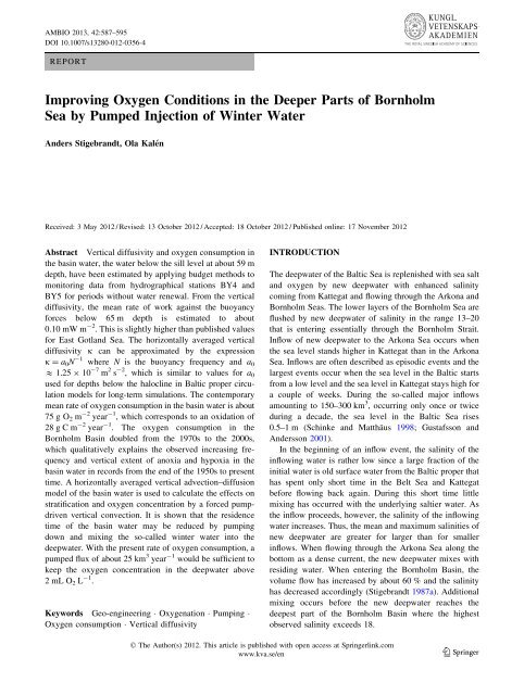
AMBIO 2013, 42:587–595DOI 10.1007/s13280-012-0356-4REPORTImproving Oxygen Conditions in the Deeper Parts of BornholmSea by Pumped Injection of Winter WaterAnders Stigebrandt, Ola KalénReceived: 3 May 2012 / Revised: 13 October 2012 / Accepted: 18 October 2012 / Published online: 17 November 2012Abstract Vertical diffusivity and oxygen consumption inthe basin water, the water below the sill level at about 59 mdepth, have been estimated by applying budget methods tomonitoring data from hydrographical stations BY4 andBY5 for periods without water renewal. From the verticaldiffusivity, the mean rate of work against the buoyancyforces below 65 m depth is estimated to about0.10 mW m -2 . This is slightly higher than published valuesfor East Gotland Sea. The horizontally averaged verticaldiffusivity j can be approximated by the expressionj = a 0 N -1 where N is the buoyancy frequency and a 0& 1.25 9 10 -7 m 2 s -2 , which is similar to values for a 0used for depths below the halocline in Baltic proper circulationmodels for long-term simulations. The contemporarymean rate of oxygen consumption in the basin water is about75 g O 2 m -2 year -1 , which corresponds to an oxidation of28 g C m -2 year -1 . The oxygen consumption in theBornholm Basin doubled from the 1970s to the 2000s,which qualitatively explains the observed increasing frequencyand vertical extent of anoxia and hypoxia in thebasin water in records from the end of the 1950s to presenttime. A horizontally averaged vertical advection–diffusionmodel of the basin water is used to calculate the effects onstratification and oxygen concentration by a forced pumpdrivenvertical convection. It is shown that the residencetime of the basin water may be reduced by pumpingdown and mixing the so-called winter water into thedeepwater. With the present rate of oxygen consumption, apumped flux of about 25 km 3 year -1 would be sufficient tokeep the oxygen concentration in the deepwater above2mLO 2 L -1 .Keywords Geo-engineering Oxygenation Pumping Oxygen consumption Vertical diffusivityINTRODUCTIONThe deepwater of the Baltic Sea is replenished with sea saltand oxygen by new deepwater with enhanced salinitycoming from Kattegat and flowing through the Arkona andBornholm Seas. The lower layers of the Bornholm Sea areflushed by new deepwater of salinity in the range 13–20that is entering essentially through the Bornholm Strait.Inflow of new deepwater to the Arkona Sea occurs whenthe sea level stands higher in Kattegat than in the ArkonaSea. Inflows are often described as episodic events and thelargest events occur when the sea level in the Baltic startsfrom a low level and the sea level in Kattegat stays high fora couple of weeks. During the so-called major inflowsamounting to 150–300 km 3 , occurring only once or twiceduring a decade, the sea level in the Baltic Sea rises0.5–1 m (Schinke and Matthäus 1998; Gustafsson andAndersson 2001).In the beginning of an inflow event, the salinity of theinflowing water is rather low since a large fraction of theinitial water is old surface water from the Baltic proper thathas spent only short time in the Belt Sea and Kattegatbefore flowing back again. During this short time littlemixing has occurred with the underlying saltier water. Asthe inflow proceeds, however, the salinity of the inflowingwater increases. Thus, the mean and maximum salinities ofnew deepwater are greater for larger than for smallerinflows. When flowing through the Arkona Sea along thebottom as a dense current, the new deepwater mixes withresiding water. When entering the Bornholm Basin, thevolume flow has increased by about 60 % and the salinityhas decreased accordingly (Stigebrandt 1987a). Additionalmixing occurs before the new deepwater reaches thedeepest part of the Bornholm Basin where the highestobserved salinity exceeds 18.Ó The Author(s) 2012. This article is published with open access at Springerlink.comwww.kva.se/en 123

588 AMBIO 2013, 42:587–595Only the densest new deepwater may reach down to thegreatest depth in the Bornholm Sea. Less dense inflows areinterleaved in the halocline (pycnocline) usually in the depthrange 50–70 m. High-saline water from large inflows mayreside for several years in the deeper parts of the BornholmSea, which has a maximum depth of about 100 m. The StolpeChannel, with sill depth 59 m, permits halocline water to exitthe Bornholm Basin and flow into the East Gotland Sea.The frequency of exchange of basin water is generallydetermined by the density range of the new deepwater andthe rate of vertical density reduction in the basin due tovertical mixing. A large density range of the new deepwatertends to give long residence times in the deeper partsof the basin water, while large rates of vertical mixing tendto give short residence times as explained in Stigebrandt(2012). The frequency of occurrence as well as the verticalextent of hypoxia and anoxia in the basin water increasewith both the residence time of the basin water and the rateof supply of organic matter.In this paper we show that the rate of density reductionin the basin water may be increased artificially by forcedmixing, e.g., by pumping less dense water from higherstrata into the basin water. This will lead to an increasedfrequency of water exchange and a decreased residencetime of basin water. In addition, pumping will also lead toan increased supply of oxygen to the deepwater. Botheffects will raise the minimum concentration of oxygen inthe basin water as demonstrated by our model simulations.Raising the oxygen content and decreasing the density ofthe Bornholm Sea basin water would imply that the Balticproper east of Bornholm Sea will receive water of higheroxygen concentration and lower salinity during the socalledmajor inflows which would help to improve theoxygen conditions in the Baltic proper. This paper isstructured as follows: we first describe the oceanographicconditions in Bornholm Sea. Then a description of thetheory used for computations in this paper is given andfinally we show the results for our computations of verticaldiffusivity and oxygen consumption in the basin water withthe pumping applied, followed by a discussion.Topography and Hydrography of the Bornholm SeaThe Bornholm Sea, situated east of the island of Bornholm,has a maximum depth of about 100 m. In the east it isconnected to East Gotland Sea by Stolpe Channel, with amaximum depth of about 59 m, see the topographical mapin Fig. 1. There is also a 46 m deep connection to the WestGotland Basin by a trench southeast of Öland. The BornholmChannel, northwest of Bornholm, is the main inlet ofnew deepwater to Bornholm Sea. It is about 40 m deep inthe west with increasing depth towards the east. A submarineridge, with maximum depth of about 29 m, runningtowards southwest from Bornholm provides the westernborder between the Bornholm and Arkona Seas (Fig. 1).Most of the new deepwater from the Arkona Sea enter theBornholm Sea through the Bornholm Channel. Only duringthe so-called major inflows some new deepwater may spillacross the shallower southern ridge (Stigebrandt 1987a;Lass et al. 2001).Fig. 1 Left panel Map of the Baltic Sea. Names mentioned in thepaper are shown in the map; a The Great Belt, b Öresund, c BornholmChannel, d Stolpe Channel, e Öland Channel. Right panel A close-upshowing the bathymetry, using the spherical grid topography of theBaltic Sea by Seifert et al. (2001). The locations of the monitoringstations BY4 and BY5 are indicated by the white circle and cross,respectively. The domain of the advection–diffusion model is givenby the white rectangle123Ó The Author(s) 2012. This article is published with open access at Springerlink.comwww.kva.se/en

AMBIO 2013, 42:587–595 589The spherical grid topography of the Baltic Sea bySeifert et al. (2001) was used to compute the hypsographicfunction, i.e., the horizontal area of the basin at differentdepths. The basin used for the computations is the rectangularregion bound by the coordinates 54.00°N, 14.25°Eand 56.21°N, 16.75°E, shown by the white rectangle inFig. 1. The horizontal surface area of Bornholm Basin isabout 14 150 km 2 at sill level (59 m) and the volume belowthe sill is about 200 km 3 .Hydrographical observations of temperature, salinity,and oxygen concentration from the period 1957 to 2011from the monitoring stations BY4, located at 55.38°N,15.33°E, and BY5 at 55.25°N, 15.98°E, see Fig. 1, wereused for this study. The numbers of unique dates of measurementsused in the series from BY4 and BY5 were 352and 433, respectively.The salinity in the Bornholm Sea is rather constant fromthe surface down to the halocline from where it increasesrapidly with depth (Fig. 2a). The vertical location of thehalocline is influenced by the depth of the Stolpe Channel.This is the reason why the halocline is closer to the seasurface in Bornholm Sea than in the main part of the Balticproper. The top of the halocline stands highest in connectionwith major inflows of new deepwater.The isopleth diagram for salinity at BY5 (Fig. 2a) showsthat the salinity in the deeper part of the basin increasesrapidly in a number of events due to inflow of new densedeepwater. Between these events the salinity decreasesslowly due to vertical diffusion. This suggests that theresidence time of water in the lower part of the basin can beseveral years. This impression is strengthened by the isoplethdiagram of oxygen (Fig. 2b), showing that deepwaterrenewals increase the oxygen concentration in the deepwater,but after a few years the oxygen is exhausted andanoxia occurs.Since the beginning of the 1980s, the oxygen concentrationis often less than 2 mL L -1 (1 mL & 44.6 lmol) below70 m depth. Anoxia seems to have occurred at BY5 for thefirst time about 1980 and since then on several occasions.Oxygen diffusion from above is obviously not sufficient tosupply all the oxygen needed for respiration at the greatestdepths. This suggests that oxygen consumption by respirationhas increased rapidly from the 1960s to the 1980s.MATERIALS AND METHODSVertical Mixing and Buoyancy Fluxes in the BasinWaterThe water of isolated basins may be treated as one-dimensionalif horizontal gradients are much smaller than vertical.We first consider circulation caused by vertical mixing andinflows of new deepwater. The one-dimensional verticaladvection–diffusion equation for salt is then an appropriatestarting point. Consider a horizontal slice (slab) of a basinFig. 2 Isopleth diagram of salinity (a) and oxygen (mL L -1 )(b) at BY5 from 1957 to 2010Ó The Author(s) 2012. This article is published with open access at Springerlink.comwww.kva.se/en 123

590 AMBIO 2013, 42:587–595centered at the depth z (Fig. 3). The slice has thickness dz,horizontal surface area A(z), volume V(z) = A(z)dz, andsalinity S = S(z). Water exchange with neighboring basinsintroduces flows q = q(z) into and out of the basin which inturn introduce vertical advection of velocity w(z). Thesalinity of water flowing into the slab by the flow q(z) isS in (z). For horizontal flow out of the slab (q is negative) S inequals S(z). Salt is also transported through the horizontalboundaries of a slab due to vertical turbulent diffusion.If the vertical z-coordinate is positive upwards, conservationof salt in the slab is described byoSot ¼ 1 AoozAj oS ooz oz ðwASÞþqS inConservation of volume requires that: ð1Þoq ðwAÞ ¼0:oz ð2ÞIf non-conservative substances like dissolved oxygenare considered, there must be a sink term in the equation asdiscussed below. The vertical advection–diffusion modelabove is discussed in, e.g., Stigebrandt (1987b, 1990).Observations in fix points show turbulence as high-frequencyfluctuations of, e.g., velocity, salinity, temperature,and other state variables. The vertical flux of, for instance,sea salt may be estimated as the time average of the productof the fluctuating components w 0 and S 0 of the verticalvelocity and the salinity, respectively. It is common todescribe the turbulent vertical flux of a scalar as a product ofthe vertical turbulent or eddy diffusivity j and the verticalgradient of the scalar. For a given locality, it is reasonable toassume that the same value of j may be used to computevertical turbulent transports of different scalars. Thus, forvertical fluxes of salt S and temperature T one obtainsj oSoz ¼ w0 S 0ð3Þj oToz ¼ w0 T 0ð4ÞSimilar expressions can be formulated for vertical fluxesof other scalars.Vertical fluxes of buoyancy tend to change the stratificationand have crucial dynamical significance. Buoyancyis denoted g 0 = gq 0 /q 0 , where g is the acceleration ofgravity, q 0 the fluctuating part of the density and q 0 areference density. An equation for the turbulent flux ofdensity w 0 q 0 may be obtained using the equation of state forseawaterq ¼ q 0 ð1 aT þ bSÞ ð5ÞHere q is density, a the coefficient of heat expansion,and b the coefficient of salt contraction. By multiplyingEq. (3) and Eq. (4) byq 0 b and q 0 a, respectively, and usingFig. 3 A horizontal slice (slab) of a fjord basin centered at depth zEq. (5), the following equation may be obtained after somealgebraic operationsj oqoz ¼ w0 q 0ð6ÞThe buoyancy flux b ¼ w 0 g 0 is obtained if Eq. (6) ismultiplied by g/q 0 , thusw 0 g 0 ¼ j N 2ð7ÞHere N 2 =-(g/q 0 )(qq/qz) is the buoyancy frequency.The buoyancy flux b also expresses the rate of work againstthe buoyancy forces (per unit mass, i.e., W kg -1 )performed by mixing processes in stratified fluids.During stagnant conditions in closed basins, changes ofsalinity and other conservative substances occur exclusivelydue to vertical diffusion, i.e., q = 0andw = 0. The horizontallyaveraged diffusion equation for salt, Eq. (1), then readsoSot ¼ 1 Ao oSAjoz ozð8ÞHere A(z) is the horizontal area of the basin.In this case horizontally averaged values of j may beestimated from horizontally averaged vertical profilesmeasured at two different occasions. Vertical integration ofEq. (8) from the greatest depth z = d, where there is nodiffusive flux of mass (through the sea bottom), to somelevel z = u, gives the following expression for the verticaldiffusivity at the level z = u:j z¼u ¼ A oS 1ozZ uz¼udoSot Adzð9ÞThis equation may be used to compute j at n - 1 levels ifthere are n levels of measurements of S = S(z,t). To obtainsignificant changes of S(z,t), the time interval between themeasurements usually must be of the order of several weeksin order to get significant changes of the state variables. Thismethod to estimate horizontally averaged j, the so-calledbudget method, is described at length by, e.g., Gargett(1984). Note that estimates of j using the budget method aretrue horizontal averages. They are independent of the valueof the coefficient of mixing efficiency Rf (the fluxRichardson number), which is not the case for estimates ofj using observations of dissipation.123Ó The Author(s) 2012. This article is published with open access at Springerlink.comwww.kva.se/en

AMBIO 2013, 42:587–595 591Application of the budget method to cases where all thesmall-scale turbulence is located in a thin layer near thebottom (boundary mixing) is discussed in Stigebrandt(1976). The budget method to estimate the vertical diffusivityhas been applied to numerous fjord basins, e.g.,Stigebrandt and Aure (1989) and to the Baltic proper by, e.g.,Axell (1998) and Gustafsson and Stigebrandt (2007).The total rate of work against the buoyancy forces, P B ,bymixing processes below the level z = h (h deeper than the silllevel) in a basin is obtained by integrating the buoyancy flux,b = jN 2 , from the greatest depth z = d to the level z = h:P B ¼Z hdq 0 jðzÞN 2 ðzÞAðzÞdzð10ÞThus, P B can be computed from Eq. (10) if the horizontalmean diffusivity j(z) has been determined. To compare thebuoyancy fluxes in various basins, one may divide P B by thearea of the basin at the upper integration limit h. This givesthe normalized power W(h) = P B /A(h) spent to buoyancyfluxes in the basin water beneath the depth h.Oxygen Consumption in the Basin WaterOne may apply the budget method also to biologicallyactive substances like nutrients and oxygen if a sink (orsource) term is added to Eq. (8), e.g. Gustafsson andStigebrandt (2007). If c m is the spatial mean concentrationof the substance in the volume V below z = u and U is thespecific source (or sink), expressed as a flux per unit horizontalsurface area, one obtainsV dc mdt¼jA dcdzþAðz ¼ uÞUz¼uð11ÞIn Eq. (11), changes of the inventory are due to bothsources (sinks) and vertical diffusion through the upperhorizontal surface at z = u. To apply the equation, thevertical diffusivity j at z = u must be estimated by usingEq. (9) on the observed concentrations of sea salt oranother conservative substance.Density Reduction by Pumping Less Dense WinterWater into the Basin WaterIf water flowing into the basin is denser than resident basinwater, it will form a dense plume-like bottom current. Thisentrains ambient water at the rate -q, i.e., there is anoutflow from the slab to the plume, whereby the volumeflow of the plume increases with depth.The combination of Eqs. (1) and (2) gives the followingequation for the rate of change of salinity of a slab in abasin with a dense bottom current:oSot ¼ 1 AoozAj oS ozþ wA oSoz þ qðS inSÞð12ÞThis can also be applied to a basin with a verticalbuoyant plume induced by pumping. Then q is the flow outof/into the slab caused by the entraining plume. At depthswhere the plume entrains ambient water, q is negativewhereas at the depth where the plume is interleaved intothe fjord basin, q is positive.The plume flow is computed as follows. A certain volumeflow Q 0 is pumped from the level z = u down to z = lwhere it is discharged in the form of horizontal jets. Acertain entrainment flow q(l) is initiated by the kineticenergy of the jets:qðlÞ ¼a Q 0ð13ÞThe entrainment coefficient a depends on the kineticenergy of the jets and is typically in the interval (0\a\10).The time step Dt used in the computation is not allowedto be so large that more than half of the water in a layer isentrained, thusDt qz ðÞ\AðÞDz=2zð14ÞHere Dz is the vertical resolution of the computationalgrid so that A(z)Dz is the volume of the slab.The flow of the plume after the initial mixing equalsQ ¼ Q 0 ð1 þ aÞð15ÞThe salinity SP and temperature TP of the plume afterinitial mixing equalsSPðÞ¼ l ðSuð ÞþaSðÞlÞ=ð1 þ aÞ ð16ÞTPðÞ¼ l ðTuð ÞþaTðÞlÞ=ð1 þ aÞ ð17ÞIf the density of the plume qP(l) is less than the densityof the water in the level next above, i.e., qP(l)\q(l - 1),the plume will move upwards under entrainment and theentrained flow equalsqðz 1Þ ¼E Q ð18ÞHere E is the coefficient of entrainment for buoyancyplumes. The new salinity and temperature of the plumewhen reaching the level z - 1 are given bySPðz 1Þ ¼ ðSPðÞþES z ðz 1ÞÞ=ð1 þ EÞ ð19ÞTPðz 1Þ ¼ ðTPðÞþET z ðz 1ÞÞ=ð1 þ EÞ ð20ÞIf the density of the plume is less than the density of theambient water on the next level above (z - 2) convectioncontinues. Otherwise the plume is interleaved at the levelz - 2. Note that the water volume to interleave Q int equalsQ int ¼ Xt lqðzÞþQ 0ð21ÞÓ The Author(s) 2012. This article is published with open access at Springerlink.comwww.kva.se/en 123

592 AMBIO 2013, 42:587–595The value of q(z) is now known and new salinities andtemperatures of the ambient basin water may be computedusing Eq. (12).If the model is used to simulate the evolution of a nonconservativesubstance the appropriate source (sink) has tobe added to Eq. (12), as discussed earlier. In the presentpaper, a simplified description of the jet and plume usingconstant values of a and E is used for simplicity.RESULTSThe budget methods to estimate the vertical diffusivity andthe rate of oxygen consumption described above, requirestagnation periods when vertical advection is negligible. Tomake sure that no inflow of dense water by a bottom currenthas occurred during the time between two consecutivemeasurements, two criteria were used. The first is that thesalinity at the greatest depth must decrease with time, qS/qt\0, owing to vertical diffusion. An inflow of densewater would increase the density and likely also the salinityof the basin water. During times of no inflow, the consumptionof oxygen by biological and geochemical processeswill decrease the content of oxygen in the basinwater. Accordingly, the second criteria for a stagnationperiod with negligible vertical advection is that the oxygenconcentration should decrease with time, qO 2 /qt\0. In ouranalysis of data from Bornholm Sea we require that bothconditions are satisfied.Vertical Diffusivity and Buoyancy FluxesThe vertical diffusivity j was estimated for stagnationperiods as described above. It was determined for thevolume below depths h equal to 65, 75, and 85 m,respectively. Calculations were done using data from BY4and BY5 separately. As expected, the results using datafrom these two stations are quite similar because observationsare from the same water mass, see Fig. 1. Averagevertical diffusivity at the three levels is given in Table 1.From the vertical diffusivity and the actual vertical stratificationwe have computed the total rate of work against thebuoyancy forces by mixing processes, P B , using Eq. (10).In Table 1 we give W = P B /A(h) which is the normalizedwork against the buoyancy forces below the depth h.The variability of all quantities in time is quite largewhich mirrors how the turbulent activity is forced by thewind which varies between different stagnation periods.There is a clear minimum in W(85) in summer, 37 versusabout 57 lWm -2 during the other seasons (not shown),supporting the conclusion by Axell (1998) that the wind isthe major energy source for the turbulence beneath thehalocline. It is not clear by which mechanisms energy istransferred to turbulence in the basin water, c.f. the discussionat the end of this paper.It is common to relate j to N by the following relationship:j ¼ a 0 N 1ð22ÞHere a 0 is an empirical intensity factor (velocity squared)accounting for the mean mixing activity of turbulence. Usinga vertical advection–diffusion filling-box model with anentraining dense bottom current carrying new deepwater intothe basin, Stigebrandt (1987b) estimated a 0 = 2.0 (± 0.7) 910 -7 (m 2 s -2 ) for the Baltic proper. Modern circulationmodels for the Baltic proper use j described by Eq. (22) witha 0 = 1.5 9 10 -7 (m 2 s -2 ) (e.g., Meier 2001; Gustafsson2003; Omstedt 2011).Oxygen ConsumptionOxygen consumption was estimated for stagnation periods,the number of such periods increases with depth and is 11for the volume below 65 m and 85 for the volume below85 m, see Table 1. The average rate of oxygen consumptionis about 75 g O 2 m -2 year -1 , which corresponds tooxidation of about 28 g C m -2 year -1 . However, there arelarge variations between the estimates as shown by thelarge standard deviation. Our analysis for the volumebelow 85 m shows that the oxygen consumption in theperiod 1970–1979 is 27.2 g m -2 year -1 increasing to58.0 g m -2 year -1 in the period 2000–2009. The increasingfrequency of anoxia from the end of the 1950s to thepresent, Fig. 2, qualitatively confirms that there is a trendwith increasing oxygen consumption.Table 1 Averages and standard deviations of vertical diffusivity j(m 2 s -1 ) at depth h (m), work W (W m -2 ) against the buoyancyforces below the depth h, a 0 (m 2 s -2 ) (see Eq. 10) at the depth h andoxygen consumption O 2 Cons (g m -2 year -1 ) below the depth h inthe Bornholm Sea based on hydrographical data from BY4 and BY5.No. j is the number of estimates of vertical diffusivity and No. O 2 isthe number of estimates of oxygen consumptionh j No. j W a 0 O 2 Cons No. O 265 2.5 ± 1.7 9 10 -6 12 1.0 ± 0.5 9 10 -4 1.1 ± 0.8 9 10 -7 74 ± 42 1175 4.5 ± 3.6 9 10 -6 35 0.7 ± 0.5 9 10 -4 1.3 ± 0.9 9 10 -7 77 ± 61 3185 8.0 ± 7.2 9 10 -6 88 0.4 ± 0.4 9 10 -4 1.4 ± 1.3 9 10 -7 50 ± 40 85123Ó The Author(s) 2012. This article is published with open access at Springerlink.comwww.kva.se/en

AMBIO 2013, 42:587–595 593Model Simulation of a Stagnation PeriodThe vertical advection–diffusion model described abovewith the state variables salinity, temperature, and oxygenwas applied to the lower parts of the Bornholm Sea. Verticaldiffusivity was computed using Eq. (22) with a 0changing with depth according to Table 1. The verticalvariation of the oxygen consumption applied in the modelis according to observations given in Table 1. The modelwas run for a stagnation period in the basin water thatstarted with unusually high salinity. Figure 4 (upper panels)shows the development of the salinity as observed (left)and according to the model run (right). The observationsshow a large oscillation in November 2003 but there doesnot seem to be any exchange of water in the lower layers.The salinity in the model develops approximately as in theobservations. Figure 4 (lower panels), shows that the evolutionsof observed and modeled oxygen are rather similar.A simulation with halved oxygen consumption, intended toshow conditions before the 1980s, shows high oxygenconcentrations at the end of the simulation period (Fig. 5).This is qualitatively in accordance with observations fromthat period.Changing Hydrography and Oxygen Conditions byPumpingWe then implemented a pump in the model that takes waterfrom 40 m depth, where there is always cold so-calledwinter water present, and releases it as horizontal jets at90 m depth. The initial entrainment by the jets is ten timeslarger than the pumped flow (a = 10). The value of theentrainment factor E = 0.05 is adopted from a similarpumped flow in Byfjorden (Liljebladh and Stigebrandt,unpubl.). For a pumped flow Q = 800 m 3 s -1 , Fig. 6 showsthat the minimum oxygen concentration equals about2.75 mL O 2 L -1 and the salinity is about 15.25 afterslightly less than 1 year of pumping. The rate of salinityreduction approximately doubles due to the pumping and atthe same time the diffusion of oxygen increases so that therate of change of oxygen is similar to that in the 1960s (c.f.Fig. 5) a time period when the observed oxygen conditionsalways were good. In the model, we have not implementedany inflow of new deepwater due to the reduction of thedensity of the basin water. However, an inflow wouldlikely appear in the later part of the pumping periodbecause the deepwater salinity almost never reaches suchlow values as 15.25 before an inflow occurs, c.f. Fig. 2.Itistherefore suggested that this rate of pumping should keepthe basin water well oxygenized with the contemporaryrate of oxygen consumption.DISCUSSIONThe time-averaged work against the buoyancy forces in thebasin water of the Bornholm Sea, 100 lWm -2 is abouttwice the value for the East Gotland Sea and slightly lessthan half the value for Landsort Deep as determined byAxell (1998). In all three locations the work against thebuoyancy forces has a seasonal cycle with minimum valuesin summer which should be a typical feature of mixingprocesses driven by the wind. Since the mean thickness ofthe basin water below 65 m equals 12 m, the mean rate ofdissipation in the basin water equals (1.2 9 10 -8 )(1 - Rf)/Rf Wkg -1 where Rf is the fraction of the turbulent energythat is used for vertical mixing and (1 - Rf) is the fractionthat dissipates to heat. With Rf = 0.1 the mean dissipationequals 1.08 9 10 -7 Wkg -1 which is about one order ofmagnitude greater than the dissipation by interior mixingobtained by van der Lee and Umlauf (2011) in BornholmSea. This suggests that most of the mixing occurs at theboundaries (boundary mixing). Dominance of boundarymixing over interior mixing in the East Gotland Sea wasdemonstrated by Holtermann et al. (2011) and Holtermannand Umlauf (2012). The latter authors discussed mechanismsthat transfer energy to the turbulence in the basinwater and pointed to the importance of sub-inertial motions(topographic waves). Liljebladh and Stigebrandt (2000)estimated that inertial currents in the surface layer maygenerate super-inertial internal gravity waves that transfersome 0.3 mW m -2 to the deepwater. If the efficiency ofturbulence with respect to creating buoyancy fluxes equals0.1 (i.e., Rf = 0.1), the internal waves should contribute awork against the buoyancy forces amounting to30 lWm -2 , which is about 30 % of the work as estimatedabove. Nohr and Gustafsson (2009) computed the energytransfer from wind-forced barotropic currents to baroclinicwaves at topography by the same mechanism that generatesinternal tides which are known to transfer most of theenergy needed by deepwater turbulence in the ocean and infjords (e.g., Stigebrandt and Aure 1989). This mechanismmay explain the large variations in work against thebuoyancy forces between basins, which depend on thetopography and the amplitudes of fluctuating barotropiccurrents. However, the information in Nohr and Gustafsson(2009) is not sufficiently detailed to allow extraction offigures of energy transfer for the Bornholm Sea.We found that the oxygen consumption below 85 m inthe Bornholm Basin doubled from the 1970s to the period2000–2009 and noted that this is in line with the trend ofincreasing frequency of anoxia from the end of the 1950s tothe present seen in Fig. 2. The trend of increasing oxygenconsumption is most probably not a regional phenomenonbut it seems to have occurred in the whole Baltic proper.Eilola (1998) used oxygen budgets to estimate oxygenÓ The Author(s) 2012. This article is published with open access at Springerlink.comwww.kva.se/en 123

594 AMBIO 2013, 42:587–595Fig. 4 Upper panels show observed (left) and modeled (right) salinity in the basin water of the Bornholm Sea from 7 May 2003 to 21 April2004. Lower panels show observed (left) and modeled (right) evolution of oxygen (mL L -1 ) during the same periodFig. 5 Evolution of oxygen concentration (mL L -1 ) when oxygenconsumption was halved as compared to normal consumption. Thisshould be representative for the 1960s and 1970sconsumption beneath the surface layer in the Baltic proper.He found that the consumption doubled from the 1930s tothe 1980s. Sandén and Håkansson (1996) found that theobserved decrease of the Secchi depth from 1919–1939 to1969–1991, indicates a doubling of both primary productionand net production since the 1930s. An analysis of thereason for these changes is outside the scope of the presentpaper. However, it seems that land-based sources ofnutrients are generally assumed to be the cause of eutrophication,e.g., Conley (2012).The horizontal area of the deepwater in the BornholmBasin is about 1/10 of that of the whole Baltic proper. Onewould then roughly expect that the oxygen supply neededto avoid anoxic bottoms in the Bornholm Basin would beabout 10 % of that in the whole Baltic proper. Stigebrandtand Gustafsson (2007) estimated that the oxygen need forthe whole Baltic proper to avoid anoxic bottoms could becovered by the oxygen in about 10 000 m 3 s -1 of oxygensaturated winter water. The need of winter water,800 m 3 s -1 , to oxygenate the Bornholm Basin estimated inthis paper fits nicely with that estimate.The description of entrainment into jets and buoyantplumes caused by pumping was deliberately simplified inthe present application. It is, however, easy to implementdynamical models for both the jet and plume mixing, e.g.,Fischer et al. (1979).Fig. 6 Computed evolution of salinity (left panel) and oxygen (mL L -1 )(right panel) in the basin water of Bornholm Sea when pumping800 m 3 s -1 from 40 to 90 m depth. E = 0.05 and a = 10123Ó The Author(s) 2012. This article is published with open access at Springerlink.comwww.kva.se/en

AMBIO 2013, 42:587–595 595The so-called reproduction volume for cod in theBornholm Basin, defined by S[11, O 2 [2mLL -1 , andT[1.5 °C, varies strongly between different years (Hinrichsenet al. 2007). The reproduction volume will mostlikely increase when the oxygen conditions and the verticalstratification in the Bornholm Basin are changed bypumping. Oxygenation will also lead to colonization ofbottoms that are presently dead. These and other ecologicalconsequences of pumping will be reported elsewhere.Acknowledgments This work was supported by the Swedish EPAthrough contract number NV 08/307 F-255-08 (the BOX project). TheSwedish Meteorological and Hydrological Institute (SMHI) provideddata from BY4 and BY5.Open Access This article is distributed under the terms of theCreative Commons Attribution License which permits any use, distribution,and reproduction in any medium, provided the originalauthor(s) and the source are credited.REFERENCESAxell, L.B. 1998. On the variability of Baltic Sea deepwater mixing.Journal of Geophysical Research 103: 21667–21682.Conley, D.J. 2012. Save the Baltic Sea. Nature 486: 463–464.Eilola, K. 1998. Oceanographic studies of the dynamics of freshwater,oxygen and nutrients in the Baltic Sea, PhD Thesis. EarthSciences Centre Publ. A30, ISSN 1400-3813, Gothenburg,Sweden: University of Gothenburg.Fischer, H.B., J.E. List, C.R. Koh, J. Imberger, and N.H. Brooks.1979. Mixing in inland and coastal waters, 483 pp. New York:Academic Press.Gargett, A.E. 1984. Vertical eddy diffusivity in the ocean interior.Journal of Marine Research 42: 359–393.Gustafsson, B.G. 2003. A time-dependent coupled-basin model of theBaltic Sea. Report no. C47, Earth Sciences Centre. GöteborgUniversity, Göteborg, 61 pp.Gustafsson, B.G., and H.C. Andersson. 2001. Modeling the exchangeof the Baltic Sea from the meridional atmospheric pressuredifference across the North Sea. Journal of GeophysicalResearch 106: 19731–19744. doi:10.1029/2000JC000593.Gustafsson, B.G., and A. Stigebrandt. 2007. Dynamics of nutrientsand oxygen/hydrogen sulphide in the Baltic Sea deepwater.Journal of Geophysical Research 112: G02023. doi:10.1029/2006JG00030.Hinrichsen, H.-H., R. Voss, K. Wieland, F. Köster, K.H. Andersen,and P. Margonski. 2007. Spatial and temporal heterogeneity ofthe cod spawning environment in the Bornholm Basin, BalticSea. Marine Ecology Progress Series 345: 245–254. doi:10.3354/meps06989.Holtermann, P.L., L. Umlauf, O. Schmale, G. Rehder, T. Tanhua, andJ. Waniek. 2011. The Baltic Sea Tracer Release Experiment. PartI: Mixing rates. Journal of Geophysical Research – Oceans. 117:C01021. ISSN 0148-0227. doi:10.1029/2011JC007439.Holtermann, P.L., and L. Umlauf. 2012. The Baltic Sea TracerRelease Experiment: 2. Mixing processes. Journal of GeophysicalResearch 117: C01022. doi:10.1029/2011JC007445.Lass, H.U., V. Mohrholz, and T. Seifert. 2001. On the dynamics of thePomeranian Bight. Continental Shelf Research 21: 1237–1261.Liljebladh, B., and A. Stigebrandt. 2000. The contribution from thesurface layer via internal waves to the energetic of deepwatermixing in the Baltic. In Experimental studies of some physicaloceanographic processes, ed. B. Liljebladh, PhD Thesis. EarthSciences Centre, Publ. A56, ISSN 1400-3813. Gothenburg,Sweden: University of Gothenburg.Meier, H.E.M. 2001. On the parameterization of mixing in threedimensionalBaltic Sea models. Journal of GeophysicalResearch 106: 30997–31016.Nohr, C., and B.G. Gustafsson. 2009. Computations of energy fordiapycnal mixing in the Baltic Sea due to internal wave dragacting on wind-driven barotropic currents. Oceanologia 51: 461–494.Omstedt, A. 2011. Guide to process based modeling of lakes andcoastal seas, 258 pp. Berlin: Springer. doi:10.1007/978-3-642-17728-6.Sandén, P., and B. Håkansson. 1996. Long-term trends in Secchidepth in the Baltic Sea. Limnology and Oceanography 41: 346–351.Schinke, H., and W. Matthäus. 1998. On the causes of major Balticinflows—an analysis of long time series. Continental ShelfResearch 18: 67–97.Seifert, T., F. Tauber, and B. Kayser. 2001. A high resolutionspherical grid topography of the Baltic Sea, revised version.Paper presented at Baltic Sea Science Congress, November 25–29, Stockholm, Sweden, Leibniz-Inst. für Ostseeforschung,Warnemünde, Germany. www.io-warnemuende.de.Stigebrandt, A. 1976. Vertical diffusion driven by internal waves in asill fjord. Journal of Physical Oceanography 6: 486–495.Stigebrandt, A. 1987a. Computations of the flow of dense water intothe Baltic Sea from hydrographical measurements in the ArkonaBasin. Tellus 39A: 170–177.Stigebrandt, A. 1987b. A model for the vertical circulation of theBaltic deep water. Journal of Physical Oceanography 17: 1772–1785.Stigebrandt, A. 2012. Hydrodynamics and circulation of fjords. InEncyclopedia of lakes and reservoirs, ed. L. Bengtsson, R.W.Herschy, and R.W. Fairbridge. doi:10.1007/978-1-4020-4410-6.Stigebrandt, A., and J. Aure. 1989. Vertical mixing in basin waters offjords. Journal of Physical Oceanography 19: 917–926.Stigebrandt, A., and B.G. Gustafsson. 2007. Improvement of Balticproper water quality using large-scale ecological engineering.AMBIO 36: 280–286.van der Lee, E.M., and L. Umlauf. 2011. Internal wave mixing in theBaltic Sea: Near-inertial waves in the absence of tides. Journal ofGeophysical Research 116: C10016. doi:10.1029/2011JC007072.AUTHOR BIOGRAPHIESAnders Stigebrandt (&) is professor of oceanography at Universityof Gothenburg. His research interests include physical and biogeochemicalocean processes and analysis of coupled physical–biogeochemical–ecologicalmarine systems. He leads the Baltic deepwaterOxygenation project (BOX).Address: Department of Earth Sciences/Oceanography, University ofGothenburg, Box 460, 40530 Gothenburg, Sweden.e-mail: anst@gvc.gu.seOla Kalén is PhD student of oceanography at University of Gothenburg.He is interested in physical oceanographic processes, modeling,and polar oceanography.Address: Department of Earth Sciences/Oceanography, University ofGothenburg, Box 460, 40530 Gothenburg, Sweden.e-mail: ola.kalen@gu.seÓ The Author(s) 2012. This article is published with open access at Springerlink.comwww.kva.se/en 123