Covering Pareto Sets by Multilevel Subdivision Techniques

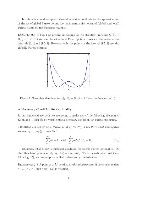
In this article we develop set oriented numerical methods for the approximationof the set of global Pareto points. Let us illustrate the notion of (global and local)Pareto points by the following example.Example 2.3 In Fig. 1 we present an example of two objective functions f j : Ê →Ê, j =1, 2. In this case the set of local Pareto points consists of the union of theintervals [0, 1] and [1.5, 2]. However, only the points in the interval [1.5, 2] are alsoglobally Pareto optimal.6543210−1 −0.5 0 0.5 1 1.5 2 2.5 3xFigure 1: Two objective functions f j : Ê → Ê (j =1, 2) on the interval [−1, 3].A Necessary Condition for OptimalityIn our numerical methods we are going to make use of the following theorem ofKuhn and Tucker ([14]) which states a necessary condition for Pareto optimality.Theorem 2.4 Let x ∗ be a Pareto point of (MOP).Then there exist nonnegativescalars α 1 ,...,α k ≥ 0 such thatk∑α i =1i=1andk∑α i ∇f i (x ∗ )=0. (2.2)i=1Obviously (2.2) is not a sufficient condition for (local) Pareto optimality. Onthe other hand points satisfying (2.2) are certainly “Pareto candidates” and thus,following [15], we now emphasize their relevance by the followingDefinition 2.5 Apointx ∈ Ê n is called a substationary point if there exist scalarsα 1 ,...,α k ≥ 0 such that (2.2) is satisfied.4