Identifying Speculative Bubbles with an Infinite Hidden Markov Model

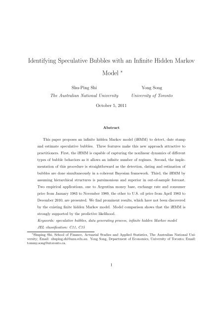
1 IntroductionBubbles, which are recognized as germs of economic and financial instability, have drawnconsiderable attention over the last several decades.specific data generating processes of bubbles has not yet been reached.Nevertheless, a general agreement onEvans (1991), forexample, recommends a periodically collapsing explosive process for bubbles. The explosivebehavior of bubbles prevails throughout the sample period, however faces a probability ofcollapsing (to a non-zero value) when it exceeds a certain threshold. If the bubble survives,it expands at a rate faster than the previous stage. 1 In contrast, Phillips et al. (2011b,PWY hereafter) propose a locally explosive bubble process in which the explosive behavior isa temporary phenomenon. Namely, asset prices transit from a unit root regime to a mildlyexplosive regime when bubbles originate and slide back to the level before origination (witha small perturbation) upon collapsing. 2Although the aforementioned processes have beenfrequently utilized as the data generating processes when comparing different econometric testsor dating algorithms for bubbles 3 , they have not been justified by any data series containingbubble episodes.This paper applies an infinite hidden Markov model (iHMM) to reconcile existing datagenerating processes within a unified and coherent Bayesian framework. This new approach isattractive to practitioners from three perspectives.First of all, the iHMM is generic to the bubble problem, since current literature assumes thatthe data dynamics in the presence of bubbles are associated with regime changes. Heuristically,Figure 1b illustrates the periodically collapsing bubble process of Evans (1991) while Figure 1cshows the locally explosive bubble behavior of PWY. One common feature is that they bothassume a fixed number of regimes a priori, hence the model uncertainty problem is ignored.One contribution of the iHMM is to provide much more flexibility by allowing an unknownnumber of regimes, which is treated as a parameter and estimated endogenously. This model1 Charemza and Deadman (1995) propose a stochastic explosive bubble process based on the periodicallycollapsing process of Evans (1991).2 Shi et al. (2011) modify the locally explosive process by replacing the one-period bubble collapsing processwith a stationary mean-reverting process.3 See Evans (1991) and Phillips et al. (2011b), among others.2

0 20 40 60 80 100(a) The non-bubble scenariotime0 20 40 60 80 100(b) The periodically collapsing explosivebehavior of Evans (1991)time0 20 40 60 80 100time0 20 40 60 80 100time(c) The locally explosive behavior of PWY(d) The hybrid bubble behaviorFigure 1: Illustration of different data generating processes of bubblesincorporates linear dynamic (Figure 1a), existing nonlinear dynamics (Figure 1a-1b), and somemuch richer dynamic with multiple and heterogeneous bubbles (Figure 1d). 4The second contribution is that we propose an easy and coherent dating algorithm for bubblesby estimating the iHMM in the Bayesian framework. One of the prevailing approachesfor date stamping bubbles 5 is the Markov-switching Augmented Dickey-Fuller (MSADF) testproposed by Hall et al. (1999, HPS hereafter). The MSADF test requires to assume or testfor state dimension before estimating the model. However, to the best of our knowledge, theperformance of testing procedures for the state dimension of a Markov-switching model which4 Phillips et al. (2011a) argues that multiples bubbles is a inherent feature of a long-span economic or financialprice series.5 Another prevailing approach is the sup type unit root test of Phillips et al. (2011b) and Phillips et al.(2011a).3

involves nonstationary (especially explosive) behavior has not yet been investigated. A subjectiveor an inaccurate selection of the state dimension may cause significant bias in parameterestimation and regime classification. Moreover, the boostrapping procedure embedded in theMSADF test is computationally burdensome as Psaradakis et al. (2001) pointed out and theasymptotic correctness of such bootstrapping procedure has not yet been established and isfar from obvious. In contrast to existing frequentists’ approaches, the Bayesian methodologyallows us to draw inference with a small sample size. The number of regimes and other modelparameters are estimated simultaneously using Markov Chain Monte Carlo methods. Thedating algorithm is then built on the posterior distributions of the iHMM’s parameters. Theimplementation of this algorithm is much less computational demanding compared with HPS.Lastly, out approach is less subjective than the iHMM of Teh et al. (2006) and Fox et al.(2011) by using two parallel hierarchical structures for the model parameters. Geweke andJiang (2011) emphasize the importance of the prior elicitation for regime change models. Oneprominent approach to dealing this problem is using hierarchical structures as Pesaran et al.(2006) among many. Simply speaking, we estimate the prior for the parameters which characterizeeach regime instead of assuming it as fixed. This methodology produces results robustto the prior choice from an empirical point of view. It is also very convenient from the computationalperspective, since regime switching may be practically infeasible with some wild prior.The hierarchical structure will shrink it to a reasonable one, hence facilitates the mixing of theMarkov chain.The first application of the iHMM is to the money base, exchange rate and consumer pricein Argentina from January 1983 to November 1989 as in HPS. It is designed to investigate ifthere exist any new discoveries after we extend the finite hidden Markov model to the infinitedimension. The two-regime Markov switching model of HPS (MS2 thereafter) is estimated inthe Bayesian framework as a benchmark. On one hand, some similarities exist between theiHMM and the MS2. On the other hand, we find new prominent features implied by the iHMM.First, the iHMM and MS2 have the same results for the money base, which are resembleto the locally explosive behavior of PWY. Second, the iHMM implies that the exchange rate’s4

dynamic is similar to to the periodically collapsing process of Evans (1991), while the MS2finds no sign of bubble collapse. Lastly, the iHMM finds evidence of bubble existence inthe consumer price throughout the whole sample period, whereas the MS2 suggests that theexplosive behaviors only appear for two short periods starting in June 1985 and July 1989,respectively.We use the predictive likelihood as the criterion for model comparison. It is based onprediction and acts as the Ockham’s razor by automatically punishing overparametrization.The results show that the two-regime specification is as good as the iHMM for the money base.However, for the exchange rate and the consumer price, the predictive likelihood stronglysupports the iHMM against the MS2. Hence, the results found by the iHMM is more crediblefrom the statistical point of view. We find the explosive money growth in June 1985 did nottrigger significant change of dynamics for the exchange rate and consumer price. On the otherhand, the explosive growth of the money base in July 1989 is associated with both the exchangerate and the consumer price switching to explosive dynamic regimes.The second application is to U.S. oil price from April 1983 to December 2010. The oilinventory is used as a proxy to the market fundamental. According to the predictive likelihoods,the iHMM fits the oil price better than the MS2. The iHMM suggests that there exist mildbubbles in the oil price during most of the sample period with four major bubble collapsingperiods following the 1985 oil price war, the first Persian Gulf War, the 1998 Asian financialcrisis and the subprime mortgage crisis. On the other hand, no explosive dynamic is discoveredin the oil inventory data.The rest of the paper is organized as follows. Section 2 introduces the infinite hiddenMarkov model. The estimation procedure, along with the dating algorithm of bubbles andthe model comparison method, are described in Section 3. The application to the Argentinahyperinflation period and the U.S oil price are in Section 4 and Section 5. Section 6 concludesthe paper.5

2 Infinite Hidden Markov ModelThe infinite hidden Markov model is expressed asy t | s t = i, Θ, Y 1,t−1 ∼ f(y t | θ i , Y 1,t−1 ), (1)Pr(s t = i | s t−1 = j, S 1,t−2 , P, Y 1,t−1 ) = Pr(s t = i | s t−1 = j, P ) = π ji , (2)where i, j = 1, 2, · · · . y t is the data at time t and Y 1,t−1 = (y 1 , · · · , y t−1 ). s t is the regimeindicator at time t and S 1,t−2 = (s 1 , · · · , s t−2 ). Θ = (θ 1 , θ 2 , · · · ) is the collection of parameterθ i ’s, which characterize each regime. P is an infinite dimensional transition matrix with π ji onits jth row and ith column. 6 (1) shows that the conditional density of y t depends on s t andthe past information Y 1,t−1 . (2) implies that the dynamic of s t only depends on s t−1 .A finite hidden Markov model (HMM) with K regimes, for instance the two-regime Markovswitchingmodel of HPS (K = 2), is nested in the iHMM by assuming K π ji = 1 for j∑=1, · · · , K, and the initial regime s 1 ∈ {1, · · · , K}. In addition, the periodically collapsingprocess of Evans (1991) and the locally explosive process of Phillips et al. (2011b) can becaptured by a three-regime HMM.In order to identify exuberant dynamics, this paper assumes (1) to have a form as of theaugmented Dickey-Fuller (ADF) test:i=1f(∆y t | θ st , Y 1,t−1 ) ∼ N(ϕ st ,0 + β st y t−1 + ϕ st, 1∆y t−1 + · · · + ∆ϕ st, qy t−q , σ 2 s t), (3)where q is the lag order and θ st = (ϕ ′ s t, σ st ) by construction with ϕ st = (ϕ st ,0, β st , ϕ st, 1, · · · , ϕ st ,q).Notice that we model ∆y t instead of y t . The existence of explosive behaviors is determined bythe coefficient of y t−1 , namely β st . A random walk process implies β st = 0 in an ADF test. Inthis paper, a positive β st shows that y t is explosive at time t.The Bayesian approach is applied in estimation to deal with infinite dimensionality. Twoparallel hierarchical priors, one governing Θ and the other governing P , are introduced as6 ∑By definition, π ji ≥ 0 for all j, i = 1, 2, · · · and ∞ π ji = 1 for all j = 1, 2, · · · .i=16

follows.2.1 Prior of ΘWe assume θ i to have the regular normal gamma distribution NG(ϕ, H, χ 2 , ν 2) (see Geweke(2009)), which is conjugate to linear models. In detail,( χσi −2 ∼ G2 , ν )2and ϕ i | σ i ∼ N ( ϕ, σ 2 i H −1) . (4)The inverse of the variance σ −2iis drawn from a gamma distribution with degree of freedom ν 2and multiplier χ 2 . Conditional on σ i, the vector of regression coefficients, ϕ i , has a multivariatenormal distribution with mean ϕ and covariance matrix σ 2 i H−1 . 7Define λ = (ϕ, H, χ, ν) as the collection of the parameters in the normal gamma distribution.A common practice for a finite hidden Markov model is to assume λ as constant. For the iHMM,however, the number of regimes can grow with the sample size, which allows us to learn λ byusing the information across regimes. Hence, we estimate it by giving it the prior as follows:H ∼ W(A 0 , a 0 ), (5)ϕ | H ∼ N(m 0 , τ 0 H −1 ), (6)χ ∼ G( d 02 , c 0),2(7)ν ∼ Exp(ρ ν ). (8)H is a positive definite matrix and drawn from a Wishart distribution. 8 Conditional on H, ϕhas a multivariate normal distribution with mean m 0 and covariance matrix τ 0 H −1 . The priorof χ is a gamma distribution with multiplier d 0 /2 and degree of freedom of c 0 /2. The prior ofν is an exponential distribution with parameter ρ ν .7 χ and ν are positive scalars. The mean and variance of σ −2i are ν 2νand , respectively. The mean of σ 2 χ χ 2 i isχ. ϕ is a (q + 2) × 1 vector and H is a (q + 2) × (q + 2) positive definite matrix.(ν−2) 8 The Wishart distribution is the extension of the gamma distribution to the multivariate setting. ParametersA 0 is a (q + 2) × (q + 2) positive definite matrix and a 0 is a positive scalar. A sample from Wishart distributionW (A 0 , a 0 ) is a positive definite matrix. The prior mean of H is A 0 a 0 . The variance of H ij , the ith row and thejth column element of H, is a 0 (A 2 ij + A ii A ij ), where A ij is the ith row and the jth column element of A 0 .7

This methodology is less subjective than Teh et al. (2006) and Fox et al. (2011) becausethe hierarchical structure is robust to prior elicitation. It also facilitates the mixing of theMarkov chain by shrinking λ to a reasonable region so that a new regime can be easily born ifa structural change is implied by the data.2.2 Prior of PThe infinite-dimensional transition matrix P is comprised of an infinite number of infinitedimensionalrow vector π j ’s, where j = 1, 2, · · · . Each π j = (π j1 , π j2 , · · · ) represents a probabilitymeasure on the natural numbers, namely, Pr(A | π j ) = ∞ π ji 1 i∈A . By definition,∑we∑should have π ji ≥ 0 for each j and i and ∞ π ji = 1 for each j. The prior of P is set asi=1i=1π 0 ∼ SBP(γ), (9)π j | π 0 ∼ DP (c, (1 − ρ)π 0 + ρδ j ) . (10)π 0 is a random probability measure on the natural numbers and drawn from a stick breakingprocess (SBP). 9 It serves as a hierarchical parameter of all π j ’s. Conditional on π 0 , each π jis drawn from a Dirichlet process (DP) with concentration parameter c and shape parameter(1 − ρ)π 0 + ρδ j . 10 The aforementioned constraints on π j ’s are automatically satisfied by thisprior.From (10), the shape parameter, (1 − ρ)π 0 + ρδ j , is an infinite discrete distribution andrepresents the mean of π j by the definition of DP. It is a convex combination of the hierarchicaldistribution π 0 and a degenerate distribution at integer j, δ j 11 , with ρ ∈ [0, 1]. The hierarchical9 The stick breaking process generates a probability measure over natural numbers. Each number is associatedwith a non-zero probability. For a probability measure p ≡ (p 1 , p 2 , · · · ) ∼ SBP(γ), where γ is a positive scalarwhich controls the concentration of a random probability measure, p i is the probability associated with integeri with i = 1, 2, · · · . Appendix A.2 provides detailed explanation of this process.10 A Dirichlet process is a distribution of discrete distributions. It has two parameters: the shape parameterand the concentration parameter. The shape parameter is a probability measure and controls the centre of therandom samples, which is analogous to the mean of a distribution. The concentration parameter is a positivescalar and controls the tightness of a random draw, which is analogous to the inverse of the variance of adistribution. Appendix A.1 provides a detailed{discussion of this process.1 if j ∈ A11 δ j is a probability measure with δ j (A) = .0 o.w.8

distribution π 0 creates a common shape for each π j and δ j reflects the prior belief of regimepersistence. By construction, conditional on π 0 and ρ, the mean of the transition matrix P isa convex combination of two infinite-dimensional matrices, expressed by⎡E(P | π 0 , ρ) = (1 − ρ) ·⎢⎣⎤ ⎡π 01 π 02 π 03 · · ·π 01 π 02 π 03 · · ·+ ρ ·π 01 π 02 π 03 · · · ⎥ ⎢⎦ ⎣.. . . ..⎤1 0 0 · · ·0 1 0 · · ·.0 0 1 · · · ⎥⎦.. . . ..The above conditional mean of P shows that the self-transition probability is larger as ρ goescloser to 1. In the rest of the paper, ρ is referred to as the sticky coefficient. It is introduced tothe iHMM for two reasons. First, empirical evidence shows that regime persistence is a salientfeature of many macroeconomic and finance variables. The sticky coefficient explicitly embedsthis feature into the prior. Second, a finite hidden Markov model usually has a small number ofregimes, which guarantees that each regime can have a reasonable amount of data. The infinitehidden Markov model, however, may assign each data to one distinct regime. This phenomenonis called state saturation, which is obviously not interesting and harmful to forecasting. Thesticky coefficient shrinks the over-dispersed regime allocation towards a coherent one and henceavoids the state saturation problem.In summary, the iHMM is comprised of (1) and (2), in which (1) takes the form of (3) forbubble detection and estimation. (4)-(8) comprise the hierarchical prior for Θ, and (9)-(10)comprise the hierarchical prior for P .3 Estimation, Dating Algorithm and Model Comparison3.1 EstimationThe posterior sampling is based on a Markov Chain Monte Carlo (MCMC) method. Fox et al.(2011) show that the block sampler which approximates the iHMM with truncation is more9

efficient than the individual sampler. 12 We approximate the iHMM by truncation with a finitebut large number of regimes. If the number of regimes is large enough, the finite approximationis equivalent to the iHMM in practice. 13Suppose L is the maximal number of regimes in the approximation, the model is as follows:( γπ 0 ∼ DirL L), · · · , γ , (11)π j | π 0 ∼ Dir ((1 − ρ)cπ 01 , ..., (1 − ρ)cπ 0i + ρc, · · · , (1 − ρ)cπ 0L ) , (12)s t | s t−1 = j ∼ π j , (13)(ϕ, H, χ, ν) ∼ G, (14)θ i ∼ NG(ϕ, H, χ 2 , ν ), (15)2∆y t | Y 1,t−1 ∼ N(ϕ st,0 + β st y t−1 + ϕ st,1∆y t−1 + · · · + ∆ϕ st,qy t−q , σ 2 s t), (16)where j = 1, 2, · · · , L and Dir represents the Dirichlet distribution. Notice that the only approximationis (11), which is from Ishwaran and Zarepour (2000). They show that Dir ( γL , · · · , γ )Lconverges to SBP(γ) as L → ∞. (12) is not an approximation, because a DP is equivalent toa Dirichlet distribution if its shape parameter only has support on a finite set. (11) and (12)comprise the prior of P . The dynamic of the regime indicator (13) is the same as (2). (14)and (15) comprise the prior of Θ, which is the same as (4) - (8) in the iHMM. The conditionaldata density (16) is the same as (1). Different L’s are tried to investigate the robustness of theblock sampler in applications.To sample from the posterior distribution, the MCMC method partitions the parameterspace into four parts: (S, I), (Θ, P, π 0 ), (ϕ, H, χ) and ν, where S and I are the collection ofregime indicators s t ’s and binary auxiliary variables I t ’s respectively. 14 Each part is randomlysampled conditional on the other parts and the data Y = (y 1 , · · · , y T ). The sampling algorithmsare as follows (see Appendix B for more details):12 Consistency proof of the approximation can be found in Ishwaran and Zarepour (2000), Ishwaran andZarepour (2002). Ishwaran and James (2001) compare the individual sampler with the block sampler and findthat the later one is more efficient in terms of mixing.13 For example, the approximation is exact if the number of regimes equals to the number of data T .14 I t is an auxiliary variable to sample π 0 . Details are in the appendix B.10

1. Sample (S, I) | Θ, P, Y(a) Sample S | Θ, P, Y by the forward filtering and backward sampling method of Chib(1996).(b) Sample I | S by a Polya Urn scheme.2. Sample (Θ, P, π 0 ) | S, I, Y(a) Sample π 0 | I from a Dirichlet distribution.(b) Sample P | π 0 , S from Dirichlet distributions.(c) Sample Θ | S, Y by the regular linear model results.3. Sample (ϕ, H, χ) | S, Θ, ν(a) Sample (ϕ, H) | S, Θ by conjugacy of the Normal-Wishart distribution.(b) Sample χ | ν, S, Θ from a gamma distribution.4. Sample ν | χ, S, Θ by a Metropolis-Hastings algorithm.After initiating the parameter values, the algorithm is applied iteratively to obtain a largenumber of samples of the model parameters. We discard the first block of the samples to removedependence on the initial values. The rest of the samples, {S (i) , Θ (i) , P (i) , π (i)0 , ϕ(i) , H (i) , χ (i) , ν (i) } N i=1 ,are used for inferences as if they were drawn from their posterior distributions. Simulation consistentposterior statistics are computed as sample averages. For example, the posterior meanof ϕ is calculated by 1 N∑ Ni=1 ϕ(i) . In order to avoid the label-switching problem in mixturemodels 15 , we use label-invariant statistics suggested by Geweke (2007) so that the posteriorsampling algorithm can be implemented without modification.15 For example, switching the values of (θ j , π j ) and (θ k , π k ), swapping the values of state s t for s t = j, k whilekeeping the other parameters unchanged results in the same likelihood.11

3.2 Dating Algorithm of BubblesThe explosive behavior of bubbles depends on the estimates of (16). The autoregressive coefficientof y t−1 (i.e. β st ) should be positive in the presence of explosive bubbles and negativewhen the data is locally stationary mean-reverting.The Bayesian approach produces the whole posterior distribution of β st instead of a pointestimate, so one can make decisions based on his/her specific loss function. This paper considerstwo intuitive posterior statistics, which are derived from two simple loss functions, to helpidentify bubbles. One is the posterior probability P (β st > 0 | Y ) and the other is the posteriormean E (β st | Y ).For the first statistic, we claim that a bubble exists at time t if the posterior probability ofβ st > 0 is above 0.5 and there is no bubble otherwise. More concisely,bubble exists in period t if P (β st > 0 | Y ) > 0.5 .It is easy to see that this criterion is derived from an absolute value loss function. The cutoffvalue can be different from 0.5 if the loss function is asymmetric.The second statistic is based on a quadratic loss function. We claim that a bubble exists ifthe posterior mean of β stis above zero and there is no bubble otherwise. More concisely,bubble exists in period t if E (β st | Y ) > 0 .This statistic also shows the magnitude of explosiveness. The higher the value is, the fasterthe bubble expanses.3.3 Model ComparisonWe use the predictive likelihood for model comparison as suggested by Geweke and Amisano(2010). Conditional on an initial data set Y 1,t , the predictive likelihood of Y t+1,T = (y t+1 , · · · , y T )12

4 Empirical Application: Argentina HyperinflationIn this section, we apply the iHMM approach to the money base, exchange rate and consumerprice in Argentina from January 1983 to November 1989. The money base is used as a proxyfor market fundamental and the exchange rate data series is to capture fundamentally determinedbubble-like behavior. The purpose is to investigate whether there is evidence of bubblebehaviors in the consumer price.These three data series are also examined in HPS and Shi (2010). Both HPS and Shi (2010)conduct a two-regime Markov-switching ADF (MSADF) test (with different specifications inthe error variance) on these three data series and conclude no evidence of bubbles in theconsumer price. The two-regime Markov-switching (MS2) models of HPS and Shi (2010) areboth estimated by MLE.As a benchmark, we estimate a MS2 model using the Bayesian approach, which is 16∆y t | s t = j, Y 1,t−1 ∼ N(ϕ j0 + β j y t−1 + ϕ j1 ∆y t−1 + · · · + ϕ j4 ∆y t−4 , σ 2 j ) (18)Pr(s t = j | s t−1 = j) = p jj (19)with j = 1, 2. The prior of self-transition probabilities p 11 and p 22 is Beta(9, 1) and the priorof (ϕ j , σ j ) is a normal-gamma distribution, namely σ −2jThe prior mean and variance of precision σ −2j∼ G(1, 1) and ϕ j | σ j ∼ N(0, σ 2 I).are unity. The infinite hidden Markov model,(11)-(16) is estimated by setting L = 5 and with priors ϕ, H ∼ NW(0, 1, 0.2I, 5), χ ∼ G(1, 1)and ν ∼ Exp(1). 17 We set this prior in order to make the prior parameters of the MS2 modelequal to the mean of the hierarchical prior of the iHMM.Figure 2 illustrates the posterior probabilities of β st> 0 (i.e P (β st > 0|Y )) for the logarithmicmoney base, exchange rate and consumer price. From the MS2 model (dotted line),we can see that the posterior probability exceeds the 0.5 in June 1985 and July 1989 for allthree data series, which suggests the existence of explosive behaviors. Meanwhile, since thespikes appear simultaneous in these two periods, the explosive behavior of market fundamentals16 The lag order is the same as that in HPS and Shi (2010).17 Larger Ls produce the same results in bubble detection.14

(money growth) is consistent with the explosive dynamics of the exchange rate and consumerprice. However, we also find bubbles in the exchange rate emerge in April 1987, October 1987and September 1988, which have some locally explosive dynamics that can not be explainedby the money base. This is further supported by the posterior mean of β st (i.e. E(β st |Y ))displayed in Figure 3.0.0 0.2 0.4 0.6 0.8money baseP(βt>0 | Data,IHMM)P(βt>0 | Data,MS2)0.2 0.4 0.6 0.80.0 0.2 0.4 0.6 0.8 1.0 1.20.0 0.2 0.4 0.6 0.8 1.0exchange rateP(βt>0 | Data,IHMM)P(βt>0 | Data,MS2)priceP(βt>0 | Data,IHMM)P(βt>0 | Data,MS2)0.2 0.4 0.6 0.8 1.0 0.5 0.6 0.7 0.8 0.91984−01 1985−01 1986−01 1987−01 1988−01 1989−01Figure 2: The growth rate and the posterior probabilities of β stexchange rate and consumer price> 0 for the money base,The posterior probability and posterior mean of the money base from the iHMM (dashedline) are identical to those from the MS2 model. Therefore, it is reasonable to have a two-regimespecification for the money base. On the other hand, the iHMM shows distinct probability andmean patterns for the exchange rate and consumer price.For the exchange rate, the posterior probability of β st > 0 implied by the iHMM in Figure 2is almost a mirror image of that by the MS2 model except in 1989. Any plunge of P (β st > 0 | Y )of the iHMM is associated with a decrease of the exchange rate, which is consistent with Evans’s(1991) bubble collapse regime. Ironically, for the MS2 model, 4 out of 5 spikes in Figure 2correspond to decreasing of the exchange rate, which is counter intuitive. This is caused by the15

0.0 0.2 0.4 0.6 0.80.0 0.2 0.4 0.6 0.8 1.0 1.20.0 0.2 0.4 0.6 0.8 1.0money baseE(βt | Data,IHMM)E(βt | Data,MS2)exchange rateE(βt | Data,IHMM)E(βt | Data,MS2)priceE(βt | Data,IHMM)E(βt | Data,MS2)0.00 0.02 0.04 0.06 0.08 0.10 −0.005 0.005 0.015 0.0250.00 0.02 0.04 0.06 0.081984−01 1985−01 1986−01 1987−01 1988−01 1989−01Figure 3: The growth rate and posterior mean of β stconsumer pricefor the money base, exchange rate andlimited number of regimes in the MS2 model. The iHMM in Figure 2 and 3 shows that thereare approximately 3 regimes: one is associated with the bubble emerging at July 1989; oneis related to the exchange rate decreasing periods starting at June 1985, April 1987, October1987 and September 1988; and one for the rest of the sample. The MS2 model clearly combinesthe first two regimes into one and produces confusing results.For the consumer price, the iHMM implies that bubbles exist throughout the whole sampleperiod in the bottom panel of Figure 2. The bottom panel of Figure 3 shows the dynamicsof the consumer price is consistent with Evans’s (1991) assumption with time-varying degreesof explosiveness. The expansion rate is relatively higher in the one and a half years spanningfrom June 1987 to August 1988, and a considerable increase occurred over the period fromMarch 1989 to July 1989. The posterior mean of β st at the peak of this episode is 0.08. Therate then dropped rapidly so that by August 1989 it was 0.01 (same as the rate before theincrease occurred). On the other hand, the MS2 is unable to capture the dynamics becauseof assuming a limited number of regimes. Although it identifies two bubble periods staring at16

Raftery’s (1995) criterion.5 Empirical Application: U.S Oil PriceThe second application investigates the existence of speculative bubble behaviors in the U.Soil price. Several papers have studied the evidence for bubbles in the oil price (among others,Phillips and Yu (2011), Sornette et al. (2009) and Shi and Arora (2011)). Although the sampleperiods and methodologies used in these papers are different, most studies have found evidenceof bubble existence.Our data is sampled from April 1983 to December 2010. The price of the nearest-monthWest Texas Intermediate futures contract, obtained from DataStream International, is usedas a proxy for the spot oil price.We deflate the oil price by U.S. Consumer Price Indexobtained from the U.S Bureau of Labour Statistics. The market fundamental is proxied bythe oil inventory, which is the ending stocks excluding Strategic Petroleum Reserve of crudeoil and petroleum products (thousand barrels) and comes from the U.S. Energy InformationAdministration.We apply both the MS2 model and the iHMM to the logarithmic real oil price and thelogarithmic oil inventory. 18 The priors are assumed to be the same as in Section 4. Theposterior probabilities of β st > 0 and the posterior mean of β st5, respectively.are presented in Figure 4 andFor the oil inventory, both models suggest that there is no evidence of explosive behavior.Namely, the posterior probabilities (posterior means) of the inventory from both models arebelow 0.5 (zero). In fact, the posterior mean of β stremains the same throughout the sampleperiod. 19 This supports that regime switching is not a feature of the oil inventory dynamic inthe sample period.For the oil price , the patterns of the posterior probability P (β st > 0|Y ) and the posterior18 For the oil inventory, we have estimated three versions of the data: the raw data, the data that is scaled by10 −5 and the log of the raw data. All results are the same for bubble detection and regime identification. So weonly report the results based on the log of the raw data.19 Notice that the posterior mean of β st from the iHMM is smaller than that from the MS2 model. This isbecause the iHMM uses hierarchical structures but the two-regime MS model does not.18

20 40 60 80 100 120Oil PriceP(β t>0 | Data,IHMM)P(β t>0 | Data,MS2)0.0 0.2 0.4 0.6 0.8 1.013.70 13.75 13.80 13.85 13.90Log oil inventoryP(β t>0 | Data,IHMM)P(β t>0 | Data,MS2)0.0 0.2 0.4 0.6 0.8 1.0198412 198709 199006 199302 199511 199808 200105 200401 200610 200907Figure 4: Posterior probabilities of β st > 0 for the logarithmic oil price and inventory20 40 60 80 100 120Oil PriceE(β t | Data,IHMM)E(β t | Data,MS2)−0.06 −0.04 −0.02 0.0013.70 13.75 13.80 13.85 13.90Log Oil inventoryE(β t | Data,IHMM)E(β t | Data,MS2)−0.3 −0.2 −0.1 0.0 0.1 0.2 0.3198412 198709 199006 199302 199511 199808 200105 200401 200610 200907Figure 5: Posterior mean of β stfor the logarithmic oil price and inventory19

mean E (β st |Y ) from the MS2 model are different from the iHMM. For the MS2 model, theposterior probabilities of β st > 0 are always smaller than 0.5 and the posterior means of β stare negative. Therefore, no evidence of bubble exists based on the MS2 model. However, theiHMM implies that the oil price dynamic is comprised of mild explosive behavior and bubblecollapse phases, which is a prominent feature and different from Evans (1991) and PWY. Formost of the sample period, the posterior mean of β st is slightly positive. There are significantfalls (below zero) in periods following the 1985 oil price war (1985M11-1986M09), the firstPersian Gulf War (1990M04-1991M03), the 1998 Asian financial crisis (1998M12-1999M08)and the subprime mortgage crisis (2008M07-2009M07).The formal model comparison is in Table 2. It reports the log predictive likelihoods forthe oil price and the oil inventory. We can see that the iHMM outperforms the two-regimeMS model for both data series. The differences of the log predictive likelihoods are 72 and 488for the log price and the log inventory respectively. The results strongly support the iHMMagainst the two-regime switching model.Table 2: Log predictive likelihoods2-regime MS modeliHMMOil price 249 321Oil inventory -2397 -1909The last 300 observations (out of 333) are use to calculatethe predictive likelihood.6 ConclusionsThis paper proposes an infinite hidden Markov model to integrate the detection, date-stampingand estimation of bubble behaviors in a coherent Bayesian framework. It reconciles the existingdata generating processes of speculative bubbles and is able to reveal the dynamic patterns ofreal data series. Two parallel hierarchical structures provide a parsimonious methodology forprior elicitation and improve out-of-sample forecasts.20

The iHMM is applied to Argentina money base, exchange rate and consumer price fromJanuary 1983 to November 1989 and U.S. oil price and oil inventory from April 1983 to December2010. The predictive likelihoods strongly support the iHMM against a finite Markovswitching model.The dynamic of the Argentina money base is similar to the locally explosive behavior ofPWY, where the explosive behavior is a transitory phenomenon. The Argentina exchange rateand consumer price, on the other hand, resemble the periodically collapsing explosive behaviorof Evans (1991), where the explosive behavior prevails throughout the sample period and therate of explosiveness is time-varying. Furthermore, we discover that the expansion of the moneysupply in July 1989 is closely related to the simultaneous regime changes of the exchange rateand the consumer price (to a regime with a faster expansion rate).For the U.S. oil price, we find that mild explosive behavior exists for most of the timeexcept 4 major bubble collapsing periods following the 1985 oil price war, the first Persian GulfWar, the 1998 Asian financial crisis and the subprime mortgage crisis. This feature is differentfrom existing data generating processes as Evans (1991) and PWY. On the other hand, regimechange is not a feature of U.S. oil inventory data.ReferencesJ. Berger. The case for objective bayesian analysis. Bayesian Analysis, 1(3):385–402, 2006.Wojciech W. Charemza and Derek F. Deadman. Speculative bubbles with stochastic explosiveroots: The failure of unit root testing. Journal of Empirical Finance, 2:153–163, 1995.S. Chib. Calculating posterior distributions and modal estimates in Markov mixture models.Journal of Econometrics, 75(1):79–97, 1996.George W. Evans. Pitfalls in testing for explosive bubbles in asset prices. The AmericanEconomic Review, 81(4):922–930, Sep. 1991.21

Ferguson. A bayesian analysis of some nonparametric problem. The Annals of Statistics, 1(2):209–230, 1973.E.B. Fox, E.B. Sudderth, M.I. Jordan, and A.S. Willsky. A Sticky HDP-HMM with Applicationto Speaker Diarization. Annals of Applied Statistics, 5(2A):1020–1056, 2011.J. Geweke. Interpretation and inference in mixture models: Simple MCMC works. ComputationalStatistics & Data Analysis, 51(7):3529–3550, 2007.J. Geweke. Complete and Incomplete Econometric Models. Princeton Univ Pr, 2009.J. Geweke and G. Amisano. Comparing and evaluating Bayesian predictive distributions ofasset returns. International Journal of Forecasting, 2010.J. Geweke and Y. Jiang. Inference and prediction in a multiple structural break model. Journalof Econometrics, 2011.Stephen G. Hall, Zacharias Psaradakis, and Martin Sola. Detecting periodically collapsingbubbles: A markov-switching unit root test. Journal of Applied Econometrics, 14:143–154,1999.H. Ishwaran and L.F. James. Gibbs Sampling Methods for Stick-Breaking Priors. Journal ofthe American Statistical Association, 96(453), 2001.H. Ishwaran and M. Zarepour. Markov chain Monte Carlo in approximate Dirichlet and betatwo-parameter process hierarchical models. Biometrika, 87(2):371, 2000.H. Ishwaran and M. Zarepour. Dirichlet prior sieves in finite normal mixtures. Statistica Sinica,12(3):941–963, 2002.R.E. Kass and A.E. Raftery. Bayes factors. Journal of the American Statistical Association,90(430), 1995.P. Müller. A generic approach to posterior integration and Gibbs sampling. Rapport technique,pages 91–09, 1991.22

M.H. Pesaran, D. Pettenuzzo, and A. Timmermann. Forecasting time series subject to multiplestructural breaks. Review of Economic Studies, 73(4):1057–1084, 2006.Peter C. B. Phillips and Jun Yu. Dating the timeline of financial bubbles during the subprimecrisis. Quantitative Economics, forthcoming, 2011.Peter C. B. Phillips, Shu-Ping Shi, and Jun Yu. Testing for multiple bubbles. SingaporeManagement University, Center for Financial Econometrics Working Paper 2010-03, 2011a.Peter C. B. Phillips, Yangru Wu, and Jun Yu. Explosive behavior in the 1990s Nasdaq: Whendid exuberance escalate asset values? International Economic Review, 52:201–226, 2011b.Zacharias Psaradakis, Martin Sola, and Fabio Spagnolo. A simple procedure for detectingperiodically collapsing rationa bubbles. Economics Letters, 24(72):317–323, 2001.GO Roberts, A. Gelman, and WR Gilks. Weak convergence and optimal scaling of randomwalk Metropolis algorithms. The Annals of Applied Probability, 7(1):110–120, 1997.J Sethuraman. A constructive definition of dirichlet priors. Statistica Sinica, 4:639–650, 1994.Shu-Ping Shi. Bubbles or volatility: A markov-switching adf test with regime-varying errorvariance. Australian National University, School of Economics Working Paper 2010-524,2010.Shu-Ping Shi and Vipin Arora. An application of models of speculative behaviour to oil prices.Australian National University, CAMA Working paper 2011-11, 2011.Shu-Ping Shi, Peter C. B. Phillips, and Jun Yu. Specification sensitivities in right-tailed unitroot testing for financial bubbles.Paper 17, 2011.Hong Kong Institute for Monetary Research, WorkingD. Sornette, R. Woodard, and W. Zhou. The 2006-2008 oil bubble and beyond. Physica A,388:1571–1576, 2009.23

Y.W. Teh, M.I. Jordan, M.J. Beal, and D.M. Blei. Hierarchical dirichlet processes. Journal ofthe American Statistical Association, 101(476):1566–1581, 2006.24

ADirichlet Process and Stick Breaking ProcessA.1 Dirichlet ProcessBefore introducing the Dirichlet process, the definition of the Dirichlet distribution is thefollowing:Definition The Dirichlet distribution is denoted by Dir(α), where α is a K-dimensionalvector of positive values. Each sample x from Dir(α) is a K-dimensional vector with x i ∈ (0, 1)∑and K x i = 1. The probability density function isi=1p(x | α) =∑Γ( K α i ) K∏i=1K∏Γ(α i )i=1i=1x α i−1iA special case is the Beta distribution, where K = 2.∑Define α 0 = K α i and X i as the ith element of the random vector X from a Dirichleti=1distribution Dir(α). The random variable X i has mean α iα 0and variance α i(α 0 −α i )α 2 0 (α 0+1) . Hence,we can further decompose α into two parts: a shape parameter G 0 = ( α 1α 0, · · · , α Kα0) and aconcentration parameter α 0 . The shape parameter G 0 represents the center of the randomvector X and the concentration parameter α 0 controls how close X is to G 0 .The Dirichlet distribution is conjugate to the multi-nominal distribution in the followingsense: ifX ∼ Dir(α),β = (n 1 , . . . , n K ) | X ∼ Mult(X),25

∑where n i is the number of occurrences of i in a sample of n = K n i points from the discretedistribution on {1, · · · , K} defined by X. Then,i=1X | β = (n 1 , . . . , n K ) ∼ Dir(α + β).This relationship is used in Bayesian statistics to estimate the hidden parameters X, given acollection of n samples. Intuitively, if the prior is represented as Dir(α), then Dir(α + β) isthe posterior following a sequence of observations with histogram β.The Dirichlet process was introduced by Ferguson (1973) as the extension of the Dirichletdistribution from finite dimensions to infinite dimensions. It is a distribution of distributionsand has two parameters: the shape parameter G 0 is a distribution over a sample space Ω andthe concentration parameter α 0 is a positive scalar. They have similar interpretation as theircounterparts in the Dirichlet distribution. The formal definition is the following:Definition The Dirichlet process over a set Ω is a stochastic process whose sample path is aprobability distribution over Ω. For a random distribution F distributed according to a Dirichletprocess DP(α 0 , G 0 ), given any finite measurable partition A 1 , A 2 , · · · , A K of the samplespace Ω, the random vector (F (A 1 ), · · · , F (A K )) is distributed as a Dirichlet distribution withparameters (α 0 G 0 (A 1 ), · · · , α 0 G 0 (A K )).Use the results form the Dirichlet distribution, for any measurable set A, the randomvariable F (A) has mean G 0 (A) and variance G 0(A)(1−G 0 (A))α 0 +1. The mean implies the shapeparameter G 0 represents the center of a random distribution F drawn from a Dirichlet processDP(α 0 , G 0 ). Define a i ∼ F as an observation drawn from the distribution F . Because bydefinition P (a i ∈ A | F ) = F (A), we can derive P (a i ∈ A | G 0 ) = E(P (a i ∈ A | F ) | G 0 ) =E(F (A) | G 0 ) = G 0 (A). Hence, the shape parameter G 0 is also the marginal distribution ofan observation a i . The variance implies the concentration parameter α 0 controls how close therandom distribution F is to the shape parameter G 0 . The larger α 0 is, the more likely F isclose to G 0 , and vice versa.26

Suppose there are n observations, a = (a 1 , · · · , a n ), drawn from the distribution F . Usen∑δ ai (A j ) toi=1represent the number of a i in set A j , where A 1 , · · · , A K is a measurable partition of thesample space Ω and δ ai (A j ) is the Dirac measure, where⎧⎪⎨ 1 if a i ∈ A jδ ai (A j ) =.⎪⎩ 0 if a i /∈ A j( n∑)n∑Conditional on (F (A 1 ), · · · , F (A K )), the vector δ ai (A 1 ), · · · , δ ai (A K ) has a multinominaldistribution. By the conjugacy of Dirichlet distribution to the multi-nominali=1i=1distribution,the posterior distribution of (F (A 1 ), · · · , F (A K )) is still a Dirichlet distribution(F (A 1 ), · · · , F (A K )) | a ∼ Dir(α 0 G 0 (A 1 ) +n∑δ ai (A 1 ), · · · , α 0 G 0 (A K ) +i=1)n∑δ ai (A K )Because this result is valid for any finite measurable partition, the posterior of F is still Dirichletprocess by definition, with new parameters α ∗ 0 and G∗ 0 , wherei=1α ∗ 0 = α 0 + nG ∗ 0 = α 0α 0 + n G 0 +nα 0 + nThe posterior shape parameter, G ∗ 0 , is the mixture of the prior and the empirical distributionimplied by observations. As n → ∞, the shape parameter of the posterior converges tothe empirical distribution. The concentration parameter α ∗ 0n∑i=1δ ain→ ∞ implies the posterior of Fconverges to the empirical distribution with probability one. Ferguson (1973) showed that arandom distribution drawn from a Dirichlet process is almost sure discrete, although the shapeparameter G 0 can be continuous.27

A.2 Stick breaking processFor a random distribution F ∼ DP(α 0 , G 0 ), because F is almost surely discrete, it can berepresented by two parts: different values θ i ’s and their corresponding probabilities p i ’s, wherei = 1, 2, · · · . Sethuraman (1994) found the stick breaking representation of the Dirichlet processby writing F ≡ (θ, p), where θ ≡ (θ 1 , θ 2 , · · · ) ′ , p ≡ (p 1 , p 2 , · · · ) ′ ∑with p i > 0 and ∞ p i = 1. TheF ∼ DP(α 0 , G 0 ) can be generated byi=1V iiid∼ Beta(1, α 0 ) (20)∏i−1p i = V i (1 − V j ) (21)j=1θ iiid∼ G 0 (22)where i = 1, 2, · · · . In this representation, p and θ are generated independently. The processgenerating p, (20) and (21), is called the stick breaking process and denoted by p ∼ SBP(α 0 ).The name comes after the p i ’s generation. For each i, the remaining probability, 1 − i−1 ∑p j ,is sliced by a proportion of V i and given to p i . It’s like breaking a stick an infinite number oftimes.j=1BBlock samplerB.1 Sample (S, I) | Θ, P, YS | Θ, P, Y is sampled by the forward filter and backward sampler of Chib (1996).I is introduced to facilitate the π 0 sampling. From (11) and (12), the filtered distributionof π j conditional on S 1,t and π 0 is a Dirichlet distribution:()π j | S 1,t , π 0 ∼ Dir c(1 − ρ)π 01 + n (t)j1 , · · · , c(1 − ρ)π 0j + cρ + n (t)jj , · · · , c(1 − ρ)π 0L + n (t)jLwhere n (t)jiis the number of {τ | s τ = i, s τ−1 = j, τ ≤ t}. Integrating out π j , the conditional28

distribution of s t+1 given S 1,t and π 0 is:p(s t+1 = i | s t = j, S 1,t , π 0 ) ∝ c(1 − ρ)π 0i + cρδ j (i) + n (t)jiConstruct a variable I t with a Bernoulli distribution⎧∑ ⎪⎨ cρ + L n (t)jiif I t+1 = 0p(I t+1 | s t = j, S 1,t , π 0 ) ∝j=1⎪⎩c(1 − ρ) if I t+1 = 1and the conditional distribution:p(s t+1 = i | I t+1 = 0, s t = j, S t , β) ∝ n (t)ji+ cρδ j (i)p(s t+1 = i | I t+1 = 1, s t = j, S t , β) ∝ π 0iThis construction preserves the same conditional distribution of s t+1 given S 1,t and π 0 . Tosample I | S, use the Bernoulli distribution:c(1 − ρ)π 0iI t+1 | s t+1 = i, s t = j, π 0 ∼ Ber(n (t)).ji+ cρδ j (i) + c(1 − ρ)π 0iB.2 Sample (Θ, P, π 0 ) | S, I, YAfter sampling I and S, write m i = ∑ I t . By construction, the conditional posterior of π 0s t=igiven S and I only depends on I and is a Dirichlet distribution by conjugacy:π 0 | S, I ∼ Dir( γ L + m 1, · · · , γ L + m L)This approach of sampling π 0 is simpler than Fox et al. (2011).Conditional on π 0 and S, the sampling of π j is straightforward by conjugacy:π j | π 0 , S ∼ Dir(c(1 − ρ)π 01 + n j1 , · · · , c(1 − ρ)π 0j + cρ + n jj , · · · , c(1 − ρ)π 0L + n jL )29

where n ji is the number of {τ | s τ = i, s τ−1 = j}.Sampling Θ | S, Y uses the results of regular linear models. The prior is:(ϕ i , σ −2i) ∼ NG(ϕ, H, χ 2 , ν 2 ).By conjugacy, the posterior is:with(ϕ i , σi−2 ) | S, Y ∼ NG(ϕ i , H i , χ i2 , ν i2 )ϕ i = H −1i (Hϕ + X ′ iY i )H i = H + X ′ iX iχ i = χ + Y ′i Y i + ϕ ′ Hϕ − ϕ ′ Hϕν i = ν + n iwhere Y i is the collection of y t in regime i. x t = (1, y t−1 , · · · , y t−q ). X i and n i are the collectionof x t and the number of observations in regime i, respectively.B.3 Sample (ϕ, H, χ) | S, Θ, νThe conditional posterior is:ϕ, H | {ϕ i , σ i } K i=1 ∼ NW(m 1 , τ 1 , A 1 , a 1 )30

where K is the number of active regimes, with which at least one data point is associated. ϕ iand σ i are the parameters of regime i.m 1 =τ 1 =A 1 =1τ0 −1 ∑+ K σi−2i=11τ −10 + K ∑(i=1A −10 +a 1 = a 0 + K.σ −2iK∑i=1(τ −10 m 0 +K∑i=1)σi −2 ϕ iσi−2 ϕ i ϕ ′ i + τ0 −1 m 0m ′ 0 − τ1 −1 m 1m ′ 1) −1The conditional posterior of χ is:χ | ν, {σ i } K i=1 ∼ G(d 1 /2, c 1 /2)with d 1 = d 0 + K ∑i=1σ −2iand c 1 = c 0 + Kν.B.4 Sample ν | χ, S, ΘThe conditional posterior of ν has no regular density form:p(ν | χ, {σ i } K i=1) ∝() K ((χ/2) ν/2 K) ν/2∏σi−2 exp{− ν }.Γ(ν/2)ρi=1νThe Metropolis-Hastings method is applied to sample ν.distribution:{with acceptance probability minν | ν ′ ∼ G( ζ νν ′ , ζ ν)Draw a new ν from a proposal}, where ν ′ is the value from the pre-1, p(ν|χ,{σ i} K i=1 )f G(ν ′ ; ζ νν ,ζ ν )p(ν ′ |χ,{σ i } K i=1 )f G(ν; ζ νν ′ ,ζ ν )vious sweep. ζ ν is fine tuned to produce a reasonable acceptance rate around 0.5, as suggestedby Roberts et al. (1997) and Müller (1991).31