Identifying Speculative Bubbles with an Infinite Hidden Markov Model

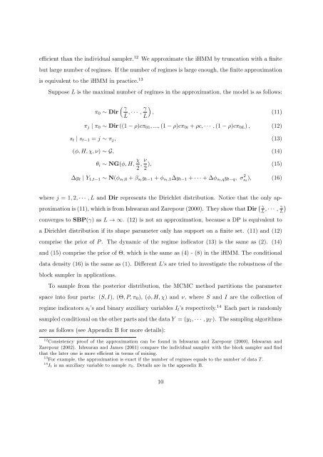
efficient than the individual sampler. 12 We approximate the iHMM by truncation with a finitebut large number of regimes. If the number of regimes is large enough, the finite approximationis equivalent to the iHMM in practice. 13Suppose L is the maximal number of regimes in the approximation, the model is as follows:( γπ 0 ∼ DirL L), · · · , γ , (11)π j | π 0 ∼ Dir ((1 − ρ)cπ 01 , ..., (1 − ρ)cπ 0i + ρc, · · · , (1 − ρ)cπ 0L ) , (12)s t | s t−1 = j ∼ π j , (13)(ϕ, H, χ, ν) ∼ G, (14)θ i ∼ NG(ϕ, H, χ 2 , ν ), (15)2∆y t | Y 1,t−1 ∼ N(ϕ st,0 + β st y t−1 + ϕ st,1∆y t−1 + · · · + ∆ϕ st,qy t−q , σ 2 s t), (16)where j = 1, 2, · · · , L and Dir represents the Dirichlet distribution. Notice that the only approximationis (11), which is from Ishwaran and Zarepour (2000). They show that Dir ( γL , · · · , γ )Lconverges to SBP(γ) as L → ∞. (12) is not an approximation, because a DP is equivalent toa Dirichlet distribution if its shape parameter only has support on a finite set. (11) and (12)comprise the prior of P . The dynamic of the regime indicator (13) is the same as (2). (14)and (15) comprise the prior of Θ, which is the same as (4) - (8) in the iHMM. The conditionaldata density (16) is the same as (1). Different L’s are tried to investigate the robustness of theblock sampler in applications.To sample from the posterior distribution, the MCMC method partitions the parameterspace into four parts: (S, I), (Θ, P, π 0 ), (ϕ, H, χ) and ν, where S and I are the collection ofregime indicators s t ’s and binary auxiliary variables I t ’s respectively. 14 Each part is randomlysampled conditional on the other parts and the data Y = (y 1 , · · · , y T ). The sampling algorithmsare as follows (see Appendix B for more details):12 Consistency proof of the approximation can be found in Ishwaran and Zarepour (2000), Ishwaran andZarepour (2002). Ishwaran and James (2001) compare the individual sampler with the block sampler and findthat the later one is more efficient in terms of mixing.13 For example, the approximation is exact if the number of regimes equals to the number of data T .14 I t is an auxiliary variable to sample π 0 . Details are in the appendix B.10