Tensor Field Visualization Using a Metric Interpretation

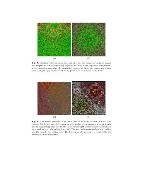
(a)(b)Fig. 7. This figure shows a single-top-load. Spot size and density of the input imagesare adapted to the corresponding eigenvectors. Red shows regions of compression,green expansion according the respective eigenvector field: the images are planarslices along the (a) yz-plane and (b) xy-plane slice orthogonal to the force.(a)(b)Fig. 8. The images represents a yz-plane (a) and xz-plane (b) slice of a two-forcedataset. (a): In the lower-left corner we see a region of compression, a result mainlydue to the pushing force on the left; in the upper-right corner expansion dominatesas a result of the right pulling force. (b): The left circle corresponds to the pushingand the right to the pulling force. The fluctuation of the color is a result of the lowresolution of the simulation.