The Bethe/Gauge Correspondence

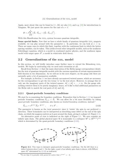
2.2. Generalizations of the xxx s model 27Again, more about this can be found in [11, §8]; see also [44], and e.g. [45] for introductions toYangians. We just quote the answer for the case of s = 1:H = JL∑ [ ⃗Sl · ⃗S l+1 − ( Sl ⃗ · ⃗S) 2 ]l+1 .l=1With this Hamiltonian the xxx 1 system becomes quantum integrable.Some special limits. Now that we have a whole family of quantum integrable xxx s magnetsavailable, we can play around with the parameter s. In particular, we can look at s → ∞.There are many ways in which this limit, together with the continuum limit in which the latticespacing vanishes, can be taken. This yields several other integrable models, such as the nonlinearSchrödinger equation, which is a model in condensed matter physics, and the nonlinear sigmamodel with target space S 2 , a model in relativistic field theory.2.2 Generalizations of the xxx s modelIn this section, we will briefly introduce some further ways to extend the Heisenberg xxx smodels. We begin by motivating why we need such extensions at all.Recall from Section 1.4 that the main observation of the Bethe/gauge correspondence identifiesthe bae of quantum integrable models with the vacuum equations of certain supersymmetricfield theories in two dimensions. As we will see in the next chapter, on the gauge side there arenaturally quite a lot of parameters available.For example, in Section 1.4 we have already encountered twisted masses, which are necessaryfor the correspondence to get the two terms ‘is’ in the bae above. However, to arrange this weonly use the imaginary parts of the twisted masses: ˜m l f= ˜m l¯f = . . . + is. On the gauge side,nothing restricts them to be purely imaginary; hence, we’d like to find additional parameters onthe Bethe side to match the real parts of ˜m l f and ˜ml¯f .2.2.1 Quasi-periodic boundary conditionsWe start by re-examining the boundary conditions. Remember that in Section 1.1.2 we imposedperiodic boundary conditions S ⃗ L+l = S ⃗ l . We can allow for a bit more flexibility by takingquasi-periodic boundary conditions, also known as twisted boundary conditions, instead: 3⃗S L+1 = e i 2 ϑ σz ⃗ S1 e − i 2 ϑ σz , ϑ ∈ S 1 . (2.22)The parameter is known as the twist parameter since it ‘twists’ the spin in our preferred z-direction. These boundaries can be interpreted as describing some defect at the end of the spinchain, on which the magnon scatters as it goes around the chain, giving it a phase (cf. Figure 2.1).An alternative point of view is indicated on the right of Figure 2.1. We now consider aninfinite spin chain. The global physical space H is isomorphic to a subspace H ϑ ⊆ (C 2s+1 ) ⊗∞which is determined by the quasi-periodic boundary conditions (2.22).Figure 2.1: Two ways to interpret quasi-periodic boundary conditions. On the left there is adefect between sites L and 1. On the right, a part of an infinite spin chain is shown, with Hilbertspace H ϑ determined by (2.22) as indicated.3 To see that ϑ is periodic with period 2π notice that e ±πiσz = − 1.