The Bethe/Gauge Correspondence

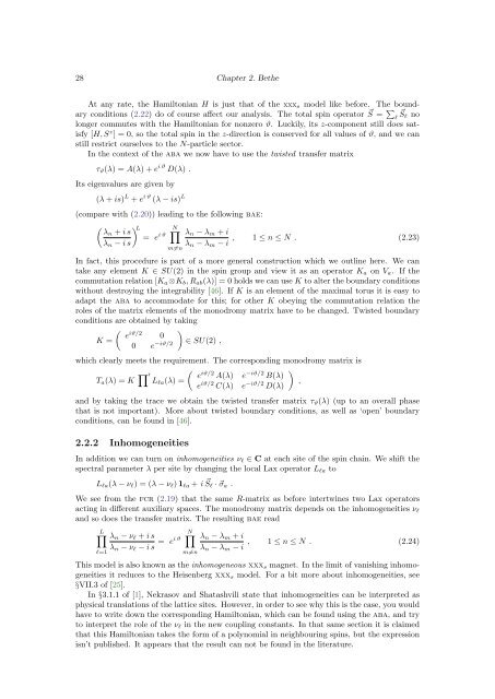
28 Chapter 2. BetheAt any rate, the Hamiltonian H is just that of the xxx s model like before. The boundaryconditions (2.22) do of course affect our analysis. The total spin operator S ⃗ = ∑ ⃗ lS l nolonger commutes with the Hamiltonian for nonzero ϑ. Luckily, its z-component still does satisfy[H, S z ] = 0, so the total spin in the z-direction is conserved for all values of ϑ, and we canstill restrict ourselves to the N-particle sector.In the context of the aba we now have to use the twisted transfer matrixτ ϑ (λ) = A(λ) + e i ϑ D(λ) .Its eigenvalues are given by(λ + is) L + e i ϑ (λ − is) L(compare with (2.20)) leading to the following bae:( ) L λn + i s ∏N= e i ϑ λ n − λ m + iλ n − i sλ n − λ m − i , 1 ≤ n ≤ N . (2.23)m≠nIn fact, this procedure is part of a more general construction which we outline here. We cantake any element K ∈ SU(2) in the spin group and view it as an operator K a on V a . If thecommutation relation [K a ⊗K b , R ab (λ)] = 0 holds we can use K to alter the boundary conditionswithout destroying the integrability [46]. If K is an element of the maximal torus it is easy toadapt the aba to accommodate for this; for other K obeying the commutation relation theroles of the matrix elements of the monodromy matrix have to be changed. Twisted boundaryconditions are obtained by taking( )eiϑ/20K =0 e −iϑ/2 ∈ SU(2) ,which clearly meets the requirement. The corresponding monodromy matrix isT a (λ) = K ∏ ( )′ eLla (λ) =iϑ/2 A(λ) e −iϑ/2 B(λ)e iϑ/2 C(λ) e −iϑ/2 ,D(λ)and by taking the trace we obtain the twisted transfer matrix τ ϑ (λ) (up to an overall phasethat is not important). More about twisted boundary conditions, as well as ‘open’ boundaryconditions, can be found in [46].2.2.2 InhomogeneitiesIn addition we can turn on inhomogeneities ν l ∈ C at each site of the spin chain. We shift thespectral parameter λ per site by changing the local Lax operator L la toL la (λ − ν l ) = (λ − ν l ) 1 la + i ⃗ S l · ⃗σ a .We see from the fcr (2.19) that the same R-matrix as before intertwines two Lax operatorsacting in different auxiliary spaces. The monodromy matrix depends on the inhomogeneities ν land so does the transfer matrix. The resulting bae readL∏l=1λ n − ν l + i sλ n − ν l − i s = ei ϑN ∏m≠nλ n − λ m + iλ n − λ m − i , 1 ≤ n ≤ N . (2.24)This model is also known as the inhomogeneous xxx s magnet. In the limit of vanishing inhomogeneitiesit reduces to the Heisenberg xxx s model. For a bit more about inhomogeneities, see§VII.3 of [25].In §3.1.1 of [1], Nekrasov and Shatashvili state that inhomogeneities can be interpreted asphysical translations of the lattice sites. However, in order to see why this is the case, you wouldhave to write down the corresponding Hamiltonian, which can be found using the aba, and tryto interpret the role of the ν l in the new coupling constants. In that same section it is claimedthat this Hamiltonian takes the form of a polynomial in neighbouring spins, but the expressionisn’t published. It appears that the result can not be found in the literature.