Line source multi tracer test for assessing high groundwater velocity

24Line source multi tracer test for assessing high groundwater velocity68Einat Magal 1, 2 , Noam Weisbrod 1 , Alex Yakirevich 1 , Daniel Kurtzman 3 and Yoseph Yechieli 2101214161 Deptment of Environmental Hydrology & Microbiology, Zuckerberg Institute for WaterResearch, Blaustein Institute for Desert Studies, Ben Gurion University of the Negev,Sede Boqer 849902 Geological Survey of Israel, 30 Malkhe Israel St., Jerusalem 955013 Institute of Soil, Water and Environmental Sciences, Agricultural Research Organization,Volcani Center, Bet Dagan 502501820Corresponding author: einat.magal@gsi.gov.il22

Abstract24A segmented line-source multi-tracer injection is suggested as an effective method forassessing groundwater velocities and flow directions in sub-surfaces characterized by high26water fluxes. Modifying the common techniques of injecting a tracer into a well becamenecessary after natural and forced gradient tracer tests ended with no reliable information on28the local groundwater flow. The tracer’s line-source increases the likelihood of success of thetest and could provide additional information regarding the lateral heterogeneity of the30aquifer.In a field experiment conducted in the northwestern part on the Dead Sea coast, tracers32were injected into an 8-m long line injection system perpendicular to the assumed flowdirection. The injection system was divided into four separate segments with four different34tracers. An array of five boreholes located within a 10x10 m area downstream was used formonitoring the tracers' transport. Two dye tracers (Uranine and Na Naphthionate) were36injected in a long pulse of several hours into two of the injection pipe segments. Two othertracers (Rhenium oxide and Gd-DTPA) were instantaneously injected into the other two38segments. The tracers were detected 0.7 to 2.3 hours after injection in four of the fiveobservation wells, located 2.3 to 10 m apart from the injection system, respectively.40The groundwater velocity was determined to be ~70-120 m/d, based on the recoveries ofthe tracers. The groundwater flow direction was derived based on the arrival of the tracers and42was found to be quite consistent with the apparent direction of the hydraulic gradient.442

Introduction46Understanding groundwater flow is essential for proper management of groundwaterresources and monitoring its quality and quantity. Water-level data is often scarce due to the48limited number of boreholes, resulting sometimes in a simplistic and non-reliable view of thegroundwater flow field. A direct estimate of groundwater flow velocity and direction is50possible by tracing the migration of a conservative tracer that has been injected artificiallyinto the aquifer. The simultaneous injection of more than one tracer into the aquifer can be52beneficial since different transport properties of the different tracers can be revealed.Monitoring the tracer concentration can be done in the injection well (dilution test) and at54observation wells downstream. The tracer test can be conducted either under the naturalhydraulic gradient or under pumping conditions (forced gradient) in order to increase the56recovery of the tracers. Tracer tests were conducted in aquifers ranging from a small scale ofmeters (Halevy et al., 1967; Molz et al., 1988) to hundreds of meters (LeBlanc et al., 1991;58Mackay et al., 1986). Tracers have been injected into aquifers through single or multipleboreholes (3-9 boreholes) at the same location (Dillon et al., 2000; LeBlanc et al., 1991;60Mackay et al., 1986; Maloszewski et al., 2003) as well as through open sinkholes and sinkingstreams (Connair and Murray, 2002; Magal et al., 2008a; Yesertener and Elhatip, 1997).62Depending on the hydraulic properties of the aquifer and the hydraulic gradient, groundwatervelocities in aquifers vary from less than a centimeter a day (Ronen et al., 1991) to a few64centimeters a day (Mackay et al., 1986; Mallants et al., 2000) and up to a few tens of meters aday (Ptak and Teutsch, 1994; Yang et al., 2001). A successful tracer test is based on a careful66and appropriate design, which requires a priori hydrogeologic knowledge of the site andpreliminary transport parameter information (Divine and McDonnell, 2005). Appropriate68selection of the tracers is also important (Magal et al., 2008b). However, this information is3

frequently not available prior to the experiment and may lead to unsuccessful tracer tests in70which there is low or no recovery of the tracer.This paper suggests a modified method of injecting tracers into the groundwater through a72line source that is separated into segments, enabling the injection of different tracers atdifferent locations. The practical benefit of the proposed method is increasing the likelihood74of recovery of tracers without a major loss of spatial information due to the relatively longsource. The arrival of the tracers injected from different locations at different observation76wells enables reconstruction of the groundwater-flow direction and a better understanding oflateral heterogeneity.78Research areaThe study was conducted in the area of the Fashkha (Zuqim) springs nature reserve, which80is located along the northwestern part on the Dead Sea coast (Figure 1a). The springs emergefrom the alluvial aquifer of the Dead Sea Group (Pliocene- Holocene) along a N-S strip of 3-482km on the western coastline of the Dead Sea. The alluvial aquifer, which is build of alterationof coarse and fine sediment, is bounded in the west by the main marginal faults of the Dead84Sea transform (Figure 1b) facing the carbonate formations of the Judea and Mt. Scopusgroups. The Fashkha springs system, together with two other groups of springs (Qane and86Samar), are the main outlets of the eastern side of the Judea Group aquifer (mountain aquifer).The hydrological system of the alluvial aquifer has been influenced by the water-level drop of88the Dead Sea during the last decades (Yechieli, 2006; Yechieli et al., 1995). Field evidenceshows a gradual process of springs drying out in the north and the appearance of new springs90in the south, in new coastal areas that were until recently covered by the Dead Sea water(Burg et al., 2006). Burg et al. (2006) suggested that a facies change in the sediment92composition from high permeability, coarse grain in the west to low-permeable sediment inthe east decreased the groundwater hydraulic connection with the receding Dead Sea and4

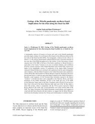
94resulted in migration of the springs southward, where coarse sediments reach very close to thepresent Dead Sea shore. The specific flow velocity and direction of the groundwater in96different parts of this hydrogeological system are questionable due to the lack of data. Kafri(2001) estimated the flow velocity of the groundwater in the Fashkha reserve, based on98radioactive decay of extremely high radon content in groundwater, to be 33-40 m/day. Thetotal discharge of the springs was estimated to be 60-70 MCM/y (Rophe, 2003) and no major100change in the springs' discharge was monitored over the years. Better understanding of thehydrological system is necessary due to the ongoing drop of the Dead Sea level, which might102risk the future of the springs as well as the natural reserve fauna and flora.104106108Figure 1: Location map and schematic cross section of the geology and hydraulic connection in theresearch area (after Burg et al., 2006).5

Material and methods110TracersTwo fluorescent dye tracers were used in the experiments: Uranine and Sodium112Naphthionate (Table 1). Both tracers were found to be of relatively low sorption affinity(Magal et al., 2008b), low toxicity (Behrens et al., 2001; Kass, 1998) and can be detected114easily with no interruptions to a minimum concentration of a few ppb. The Uranine wasmeasured in the monitoring boreholes by the CYCLOPS-7 ®submersible fluorometer of116Turner Design that was connected to the Campbell Scientific, Inc CR800 data logger, andmeasurements were taken every 10 seconds. The concentrations in ppb were computed using118the calibration line of CYCLOPS-7 ® measurements in a beaker (5 cm above the bottom) filledwith 1L of solution of known Uranine concentration (1000, 500, 100, 50, 10, 5, 1 ppb and 0).120The fluorescence intensity of Uranine is highly influenced by the solution pH (Smart andLaidlaw, 1977). Although there is no reason to believe that the groundwater pH changed122during the field experiments, the more precise results from laboratory analysis were used.Two other tracers: Rhenium oxide (Re) and Gd-DTPA (Gd) were found to be relatively124conservative (Byegard et al., 1999) and can be determined in a concentration of 0.1 ppb. Allthe tracers were purchased as dry powders and dissolved in distilled water. The dissolution of126Re 2 O 7 powder in water creates a solution of Re 2 O 4 - ions (Remy, 1956). The density of theinjected tracer-solution was kept lower than local groundwater density by 0.0005 g/cm 3128130(24°C) in order to prevent downward movement of the tracer due to density differences.Table 1: Tracers general informationTracer Commercial Name FormulaUranine Fluorescent sodium C 20 H 10 Na 2 O 5Na Naphthionate 1-Naththylamine-4-sulfonic acid C 10 H 8 NNaO 3 Ssodium salt hydrate-ReO 4 Rhenium(VII) oxide Re 2 O 7Gd-DTPA Diethylenetriaminepentaaceticacid gadolinium(III) dihydrogensalt hydrateC 14 H 20 GdN 3 O 10 xH 2 O6

Field site and experimental setup132Observation wells: five observation wells were drilled at 5-6" diameters to a depth of 10 mfor the tracer test (Figure 2). The perforated PVC pipes (2" diameter) were installed with a134gravel pack between the drilling well and the PVC pipe. The wells were drilled, using casingand without any addition of fluids (drilling mud or water). During the drilling process,136sediment samples were collected and described in the field. The sediments are composed oflayers of gravel and coarse sand alternating to layers composed of higher silt and clay138fraction. The variability in sediment composition is seen in Figure 3. In general, thepercentage of coarse sediment layers (containing more than 96% of gravel sediments) is140significantly higher than that of the fine sediments (with at least 15% of silt and clays). Themineralogical composition of the fine sediment fraction is mainly calcite, aragonite and quartz142with a minor representation of dolomite, phyllosilicates, K-feldspar and plagioclase. Quitesimilar coarse sediments with altering amounts of fines were found to the depth of 50-60 m in144two boreholes located 300 m from the experimental area (Burg et al., 2006).Groundwater samples, which were collected after pumping, had a density of 0.9999 g/cm 3146(27°C) and contained 3.0-3.6 g/l TDS (EC 5.5-6.8 mS/cm). The water level was 3.5-4 mbelow the subsurface and 6-6.5 m of the well was saturated. Based on the water level148measurements in the boreholes, an approximate value of the hydraulic gradient wasestablished to have a magnitude of 1.7% and direction of 160°N.7

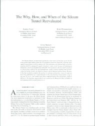
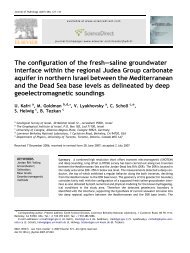
150152154Figure 2: Location map of the line-source injection system with four units (Inj 1 to Inj 4) and themonitoring boreholes (circles with numbers of the boreholes and water levels). The directionof the hydraulic gradient is marked by an arrow.156158160Figure 3: Excavated sediments at the test site channel of 4 m depth. Note the altering of sedimentcomposition from coarse and highly permeable sediment to fine and less permeable sediment.8

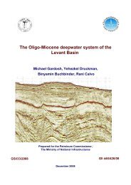
162164Line source: A line-source injection channel was excavated by backhoe to a depth of 0.2 -0.4 m below the water table (~4 m deep, 1.5 m wide and 10 m long). The dimensions of theexcavated channel were chosen because landslides prevented narrower excavation and limited166the penetration of the channel into the saturated zone to less than 0.5 m. Four units of fullyperforated pipes were installed horizontally in the excavated channel just below the water168table (Figure 4). Each horizontal pipe (2.26 m long and 4" in diameter) was connected bythree vertical non perforated PVC pipes (2" in diameter) to the surface (Figure 4). Following170the pipe installation, the channel was refilled with the same local sediments.172174Figure 4: Line-source injection pipe system. The injection pipes were installed just below the watertable. The tracers were injected through the segments as follows: Re in Inj1, Uranine in Inj2,Naphthionate in Inj3 and Gd in Inj4.Tracer test experiments176Point-injection tracer test: Two point-injection tracer tests were conducted, first on 5/3/06under conditions of a natural gradient and the second on 4/9/06 under forced gradient178conditions due to pumping. In the second experiment groundwater was pumpedcontinuously for 80 hours from well FE111 (Figure 2) at a rate of 43 L/min. The tracers9

180were injected two hours after pumping began. It is worth mentioning that during the entirepumping time, the drawdown in the pumping well was less than 3 cm. In both experiments,182two dye tracers (Uranine and Naphthionate) were injected into two boreholes, FE103 andFE110, respectively (Figure 2). Table 2 summarizes the quantities of tracers used in the184field experiments.The injection of the tracers into the wells followed a procedure described by Ward et al.186(1998) for achieving initial homogenous tracer concentration in the injection well whilekeeping steady groundwater flow during the test. In short, the procedure includes injection188of the tracer through a tube that was lowered into the bottom of the borehole. The volumeof the tracer solution was identical to the saturated part of the tube. Therefore, after lifting190the tube, tracer concentration in the ~6 m water column was relatively uniform.Preliminary laboratory investigation of a 3.5 m saturated pipe in similar spreading192conditions of the tracer found that the tracer concentration at three depths (on a 3.5 msealed tube) was similar, with a coefficient of variance of less than 7.5% between the194depths. The rate of tracer concentration dilution in the injection well was continuouslymeasured by an in-hole fluorometer. Groundwater samples of 15 ml volume were taken196using a Masterflex ® E/S TM peristaltic pump connected to 2 mm tubes lowered into thewells to the different depths. During the first five days, water samples were collected198frequently (once in one to four hours) from the observation wells (from depths of 4-4.5, 6-7 and 9-9.5m) and in the following two weeks less frequently (once a day). All200groundwater samples were kept in a dark and cold environment from the time they weresampled until they were analyzed.20210

204206208210212Table 2: Summary of the mass and concentration of the tracers used in the field experimentsTracerInjectedthroughInjectedtracer mass(g)Tracersolutionvolume (l)Injectionduration(h)C 0(ppm)BHPoint injectionUranine FE103 6.49 1.85 impulse 490Naphthionate FE110 10.81 3.09 impulse 848SegmentLine source injectionReO 4 Inj1 11.5 (of Re) 10 impulse 6583Uranine Inj2 720 720 03:29 524Naphthionate Inj3 400 400 04:17 713Gd-DTPA Inj4 15 (of Gd) 15 impulse 215214Line-source tracer test: The line source experiment (20/7/08) started with the injectionof the four different tracers into the four individual segments of the line source (Table 2).216The two fluorescent dye tracers (Uranine and Naphthionate) were injected for a few hours(Table 2) by pumping tracer solution into three 2 mm diameter tubes that were lowered218into the groundwater through the injection system’s vertical pipes (Figure 4). The injectionrate of the solution of the Uranine was 224 ±38 g/hr, whereas the Naphthionate injection220was uneven in time (60-280 g/hr) due to some technical problems. Two other tracers (Gd-DTPA and ReO 4 ) were injected in a short pulse by pouring the solution into the three222vertical pipes of the injection segments. The time of injection and the amounts of tracersused are listed in Table 2. After injecting the tracers, groundwater samples were taken224every hour from the line-source injection system and from the monitoring wells at twodepths (4-4.5 and 5-6 m). The sampling procedure included collecting 15 ml groundwater226samples using the peristaltic pump connected to 2 mm tubes lowered into the wells. Allgroundwater samples were kept in a dark and cold environment from their collection to228their analysis. Sampling was maintained at a high frequency of one sample an hour the firstday, a lower frequency of a sample every 1- 4 hours was kept for the next 8 days and from230day 9 to day 14 samples were taken once a day. In the FE101 observation well, onlinemeasurement of Uranine concentrations continued for another two weeks.11

232Laboratory analysisThe fluorescent dyes were analyzed by fluorescence spectrophotometry (Cary Eclipse234Fluorescence Spectrophotometer, Varian ® , Palo Alto, CA). The concentration of the dyes wasdetermined by using calibration curves prepared by adding known concentrations of dyes to236the natural groundwater of the Fashkha springs. Re and Gd concentrations were determinedby ICP-MS, Elan DRCII (Perkin Elmer Sciex, Canada).238Data interpretationPoint dilution test240The requirements for properly designed point dilution tests are: steady groundwater flowduring the test, homogeneous distribution of the tracer through the diluted volume and lack of242vertical current in the borehole including density driven flow (Halevy et al., 1967, Drost et al.,1968, Gaspar, 1987). The injection procedure was planned to meet these requirements. The244average groundwater velocity (in the borehole, v * ) was calculated based on diluting theconcentration of a non-reactive tracer that was introduced instantaneously into a borehole that246is a function of the groundwater flux, the vertical cross section area through the center of thesaturated borehole segment (m 2 ) and the volume of this segment (Freeze and Cherry, 1979).248The average groundwater velocity in the aquifer (v) is then calculated by dividing v * by theporosity of the aquifer and the distortion factor (α), which takes into consideration the250distortion of the groundwater flow field due to the existence of the well (Drost et al., 1968).For a borehole equipped with gravel pack, the α value can be up to four (Gaspar, 1987),252though a value of 2 is widely accepted (Pitrak et al., 2007) and was adopted in the currentwork.12

254Groundwater velocity assessment from the tracer breakthrough curvesGroundwater velocity during the tracer test was assessed in this study by the following256methods:a. According to the tracer arrival time: The tracer velocity was derived by dividing the258travel distance of the tracer along the approximated groundwater flow lines by thetime of arrival of the center of weight of the tracer breakthrough curve (the recovery of260half of the tracer mass).b. Using a one-dimension transport model: The solution of the convection-dispersion262equation using the CXTFIT code (Toride et al., 1995) for estimating transportparameters was employed for modeling the tracer breakthrough curves, assuming the264distance vector between the injection line and the observation point is in the directionof flow. The initial concentration of the tracers (C 0 ) injected in short pulses (Re and266Gd) was the concentration measured in the injection pipes immediately after theinjection.268c. Using a three-dimension transport model for the tracers that were impulse injected:tracer transport in three dimensions was modeled using the solution of Lenda and270Zuber (1970) for an instantaneous injection.C( x,y,z,t)M 1=θ 8π32( t − t')22⎡ ( y − y')⎤ ⎡ − ⎤⎢⎥ ⋅ ( z z')⋅ exp −exp⎢−⎥⎣ 4Dt( t − t')⎦ ⎣ 4Dt( t − t')⎦1D Dl2t1322⎡ {( x − x')− v(t − t')}⎤⋅ exp⎢−⎥⎣ 4D( t − t')272l ⎦274(1)276Equation (1) was derived for the advection-dispersion equation describing transport of aconservative tracer of mass M (gr) that was released at once at point (x', y', z') at time t'278(hr), θ is the aquifer porosity. D l and D t are longitude and transverse dispersioncoefficients (m 2 /h), x, y and z are the coordinates of the observation well (m). The13

280distances x and y are determined assuming the flow direction is known and is 160° fromthe north. To quantify the accuracy of the model predictions, the modified index of282agreement (MIA) was used as a goodness-of-fit estimator (Legates and McCabe, 1999)together with the R 2 and 95% confidence interval for the parameters determined by284solving inverse problem.Assessment of groundwater flow direction286The possible spectrum of flow directions of groundwater can be estimated simply byconnecting the locations in which the tracers were injected to the monitoring wells where they288were recovered. A representative direction of the groundwater flow was calculated as thedirection of the vector that resulted from the addition of the velocity vectors, which were290calculated according to the arrival time, distance and direction of the line connecting thecenter of the injection interval and the observation well.292Results and discussionTable 3 summarizes the field experiments and their main outcomes. The results and294interpretations are presented below:Point-injection tracer tests296In the natural gradient test, the tracers were not detected in the monitoring wells. Tracerconcentration declines rapidly in the injection wells; loss of 99-99.9% mass during the first298two minutes of the experiment (concentrations of Naphthionate and Uranine decline from 850to 7.4 ppm and from 90 to 0.3 ppm in 2 minutes, respectively, Figure 5). The fast dilution300prevented using the first data points in calculating groundwater flow velocity since it did notfit a linear plot on the semi-log sheet (Figure 5). The last water samples contained quite low302constant concentrations of the tracer and were not used in the calculation. Therefore, thegroundwater velocity was computed with 4-5 data points only. The average groundwater flow14

304velocity was estimated to be 22±3 m/d based on the tracer's dilution curves (Table 4).However, this estimate is questionable due to the problems described above, thus other new306field experiments were conducted to gain reliable information.In the forced gradient test there was no recovery of the tracers in the pumped water or the308observation wells. The low drawdown in the pumping well (3 cm) suggests that due to naturalhigh groundwater flow rate in the study area, the maximal pumping was insufficient to distort310the natural flow regime.312314316318Table 3: Summary of field experiments and resultsField experiment Date Results Assessed groundwatervelocityNatural gradient 5/3/06 No recovery of the tracers -Forced gradient 4/9/06 No recovery of the tracersPoint dilution test 5/3/06 22 m/dLine-source injection 20/7/08 Recovery of the tracers ~100 m/d320322324Table 4: Groundwater velocity assessments based on point dilution tests under natural gradientconditionsObservation Tracer Depth Slope v * vwell(m)(m/day) (m/day)FE103 Uranine 4.5 9.0 8.6 21.57 7.4 7.1 17.7FE110Naphthionate9.5 8.8 8.4 21.07 9.6 9.2 23.09.5 11.3 10.8 27.1*the flux through the borehole influenced by distortion of the flow field into the borehole, which iscorrected for v - estimated groundwater velocity.32632815

330332a.334336338340342344346348350352354Figure 5: Tracer dilution under anatural gradient at differentdepths in the injection wells: a.Uranine (FE103), b. Naphthionate(FE111). Groundwater velocitywas calculated according to theregression lines sketched for eachcurve.356A numerical exercise was carried out in order to check whether the field conditions in the358study area can lead to a situation whereby no detectable tracer concentrations are found in themonitoring wells. The distribution of the tracer plume was evaluated using Equation 1, for360groundwater velocities of 20 and 100 m/d (see below). The longitudinal and transversedispersion coefficients were taken to be 12 and 0.6 m 2 /d (for v = 20 m/d), and 60 and 3 m 2 /d362(for v = 100 m/d), which are reasonable values for this system (as elaborated below). Figure 6demonstrates that, under the assumption of homogenous medium, the point source test may364result in no recovery of the tracers due to high groundwater velocity and low transversedispersion.36616

368370372374376378380382384386388390392394396400402404406408398Figure 6: Numerical experiment testing the possible dimensions of the expected plume and thechances for success of a point-source tracer test. Uranine concentrations calculated with Equation 1,for point injection into the FE103 borehole (contour values in ppb). A snapshot of the Uranine plumeis plotted for: A. Four hours after injection for groundwater velocity of 20 m/day and dispersioncoefficients of 12 and 0.6 m 2 /d, longitude and transverse, respectively and; B. One hour after injectionfor groundwater velocity of 100 m/day and dispersion coefficients of 60 and 3 m 2 /d, longitude andtransverse, respectively. Note that under these conditions the concentrations of Uranine in theobservation wells FE110 and FE101 are too low to be detected.In the given conditions of the high groundwater flow velocity and the existing array ofboreholes there are a few possibilities for increasing the likelihood of gaining direct410information on the groundwater flow field: (1) drilling additional observation wells (betweenFE110 and FE101); (2) drilling a wide pumping well for greater pumping discharge, one that412might distort the natural flow lines towards the well; (3) to inject the tracers through a line17

ather than a point, in order to enhance the probability for tracer recovery in the monitoring414wells. This was found to be a better alternative.Line-source injection tracer test416The results of the line-source injection tracer test were much more conclusive than theprevious point-source injection. After the injection of the tracers, breakthrough curves could418be detected in four out of the five observation wells (Figures 7-10). The early arrival of thetracers at the monitoring wells, after less than one hour in some cases, was even higher than420estimated according to the dilution experiments (20 m/d). The tracers Uranine, Gd andNaphthionate arrived at the FE103 borehole (Figure 7) located close to the injection system422(2 m apart). The irregular shape of the Uranine and Naphthionate breakthrough curves is anoutcome of their uneven injection and the proximity of the observation well to the injection424system. The peak concentrations of Gd arrived at the observation well clearly after less thanone hour (Figure 7). The tracers Naphthionate, Uranine and Gd arrived at the FE110426borehole; Gd peak concentrations arrived after 2.3 hours (Figure 8). Gd was the only tracerthat arrived at the FE111 borehole (Figure 9) after 1.3 hours. The tracers Re, Uranine and428Naphthionate arrived at the FE101 borehole (Figure 10), after 2, 2.2, and 3.4 hours,respectively. No tracer recovery was detected in the FE102 borehole.430Groundwater velocityThe groundwater velocity computed directly from the time of arrival of the tracers’ center432of mass resulted in an arithmetic average of 73 and 83 m/d for a flow direction of 160° and170°, respectively, (Table 5). Groundwater velocity was also estimated by the one- dimension434transport model for impulse and long pulse injection (Table 6). Three-dimension transportmodels were used only for the analysis of the tracers Gd and Re, which were instantaneously436injected (Table 6). The average groundwater velocity, calculated by the one- and three-18

dimension models, is 82 and 120 m/d, respectively (Tables 7). Thus, this estimate is highly438reliable and is four to six times higher than the value obtained by the tracer point dilution test(Table 4).440442444446448450452454456Figure 7: Breakthroughcurves in observation wellFE103 for the line injectionsource (4 m depth).1. Uranine injected at adistance of 2.3 m.2. Naphthionate injected at adistance of 2.9 m.3. Gd injected at a distanceof 4 m.458460462464466468470472474Figure 8: C/C 0 Breakthroughcurves in observation wellFE110 (4.5 m depth):Uranine injected at adistance of 6.8m,Naphthionate injected at adistance of 7.3 m and Gdinjected at a distance of 6.5m.19

476478480482484486488490492Figure 9: The Gd C/C 0breakthrough curve inobservation well FE111,injected at a distance of8.9m.494496498500502504506508510Figure 10: Tracer C/C 0breakthrough curves inobservation well FE101 (5m depth): Uranine injectedat a distance of 9.2 m,Naphthionate injected at adistance of 10 m and Reinjected at a distance of 8m.20

512514516518520522Table 5: Assessment of the groundwater velocity derived from the line-source experiment according tothe arrival time of the tracer's center of mass.Source Observation TracerVelocity along Direction *wellflow-line of (from north)Arrival timeof peakconcentrationArrivaltime ofcenterof massCorrectedtime (forinjectionduration) 160° 170°hr hr hr m/d m/dInj1 FE101 Re 2.0 3.3 3.3 67 65 154°Inj2 FE101 Uranine 2.2 3.2 1.5 30 27 169°FE103 0.6 4 2.3 147 130 134°FE1102.5 0.8 121 87Inj3 FE101 Naph 3.4 5.5 3.4 46 42 181°FE103 0.7 4.1 2 81 75 178°FE1105.6 3.5 43 37Inj4 FE103 Gd 0.8 1.4 1.4 107 105 199°FE110 2.3 4.4 4.4 48 44 182°FE1111.3 1.4 1.4 138 122 169°Arithmetic average 83 73 171°Resultant velocity vector 96 ** 171°* Direction of the line connecting the center of the injection interval and the observation well** Resultant velocity vector length divided by 8Table 6: Groundwater velocity and the dispersivity estimations calculated from the breakthroughcurves and the analytical modelsObservation Depth Tracer Velocity a l (m) * a t (m) * R 2 MIA **well(m)(m/d)a. One dimension modelFE110 4.5 Gd 25 3 0.97FE111 4.5139 0.2 0.98FE101 5 Re 65 3.4 0.97Uranine 100 1.5 0.99b. Three dimension modelFE101 5 Re 167 ± 0.4 0.6 ± 0.03 0.038 ± 0.002 0.92 0.996.5140 ± 28 0.6 ± 0.8 0.1 ± 0.9 0.65 1FE103 4 Gd 48 ± 2 5.0 ± 0.8 0.09 ± 0.06 0.89 0.975.5 120 ± 6 0.3 ± 0.2 1 ± 1 0.94 0.98FE110 4.5 123 ± 2 0.3 ± 0.03 0.6 ± 0.2 0.92 0.916 112 ± 9 0.4 ± 0.3 0.7 ± 0.8 0.91 0.98FE1114.5 153 ± 11 5 ± 5 0.01 ± 0.06 0.96 0.97692 ± 1 0.2 ± 0.04 0.7 ± 0.2 0.79 0.79± - 95% confidence interval values* a l, a t - longitude and transverse dispersivities- D l =α l v and D t =α t v** MIA- Modified index of agreement21

The direction and lateral heterogeneity of groundwater flow524The aerial distribution of the injected tracers and their arrival to the array of boreholesenables evaluation of the general flow direction of the groundwater and the identification of526the lateral heterogeneity of the flow field. The tracers' recoveries were found to be consistentin general with the simplified picture of a hydraulic gradient of 160° towards the south528(Figure 11) as detailed below: (1) the tracer Re that was injected in the western segment(Inj1) was found only in borehole FE101 located on the western side of the field experiment530(Figure 11); (2) no tracer was detected in the FE102 borehole located in the east of theexperiment field, indicating that groundwater flow towards the east was limited; (3) the Gd,532that was injected in the eastern segment (Inj4) was the only tracer found in the easternborehole FE111 (Figure 11); and (4) the Naphthionate, which was injected from Inj3, was534found in the FE103 and FE110 observation wells located in the center of the groundwaterflow direction. The recovery of Gd (Inj4) in the FE103 and FE110 observation wells and536Naphthionate (Inj3) in the FE101 observation well (Figure 11) could have resulted fromsome migration of the tracers along the horizontal injection pipes to the west, as was evident538from the occurrence of tracers in different injection segments (Table 7). A similargroundwater flow direction (171°N) was derived from the direction of the velocity vector540calculated from the arrival times at the observation boreholes (Table 5).542544546Table 7: The concentration of the tracers in all four injection pipes during the injection.SourceRe Uranine Naphthionate GdppmInj-1 (Re) 6583 63 0.5 0.1Inj-2 (Uranine) 0.02 524 4.0 0.001Inj-3 (Naphthionate) 0 58 3500 n. d.Inj-4 (Gd) 0.0 0.01 0.2 215* Gd and Re concentrations were measured 4 and 7 minutes after the injection and Uranine and Naphthionateconcentrations were measured in the middle of the injection time22

548550552Figure 11: Map of arrival of the tracers to the monitoring wells. The dashed lines represent theapparent direction of the hydraulic gradient derived from the water head in the observationwellsThe transport of Uranine suggests a more complicated flow of the tracer, as its554breakthrough curve does not readily fit the general picture of the flow lines described above:(1) Uranine was detected in the FE110 observation well located east of the flow line from the556Inj2 segment; and (2) the concentrations of Uranine recovered in the boreholes (Figure 12a)are inconsistent with their distance from their source, namely, Uranine concentration was558three orders of magnitude higher in the remote borehole (FE101, 9.2 m apart) than in thenearby borehole (FE103, 2.3 m apart). At the same time, the peaks of Gd concentrations were560on the same order of magnitude and consistent with the distance of the observation wells fromthe source (Figure 11 and Figure 12b). This may indicate the existence of a preferential flow562path with higher hydraulic conductivity that results in faster groundwater flow in a somewhatdifferent direction than the general direction implied by the hydraulic gradient.56423

566568570572574576578580582584586588590Figure 12: A comparison of thebreakthrough curves: a. Uranine(FE101, FE103 and FE110observation wells); b. Gd (FE103,FE110 and FE111 observationwells). Note that the vertical scale ofthe breakthrough curves of Uranineis logarithmic while the scale of Gdis linear.592594Dispersivity values596The experimental result analysis can provide estimations for the tracer dispersioncoefficient, although this was not a main goal of the experiment. The longitudinal dispersivity598was evaluated in the range of 0.2 to 3 m by modeling the tracer breakthrough curves with aone-dimension model (Table 6a). The longitude dispersivities derived by three–dimension600model simulations were in a range of 0.2 to 0.6 m with two exceptional high values of 5 m(Table 6b). Yet, the fitted model values for the transverse dispersivity were non-unique and602had a wide interval of confidence (Table 6b). It is possible that the high values of thetransverse dispersivity reflect the migration of the tracer east in the line-source injection604system that was wrongly simulated by the model as high transverse dispersion. A low value of0.03 m for transverse dispersivity was suggested by the "numerical exercise" to simulate the24

606experiment results of no detectable tracer concentration in the monitoring wells after pointinjection. This is almost direct evidence placing a threshold value for the transversal608dispersivity and is therefore highly reliable. It should be noted that in these simulations only aratio of 1:20 could be used for the longitudinal and transverse dispersivity, which is lower610than the ratio of 1:10, which is most frequently used (Gelhar et al., 1992). The current lowestimates for the longitudinal dispersivity (0.2 m) are consistent with the approximate612dispersivity of 0.5 m, calculated using the empirical relation between the dispersivity valueand the experiment scale proposed by Neuman (1990).614Hydraulic conductivityThe aquifer hydraulic conductivity (K s ) was calculated to be about 1200 m/d using Darcy's616law for the measured groundwater velocity (100 m/day), the calculated hydraulic gradientbased on water heads (0.017) and porosity (0.2). The K s in the study area is in the upper618representative values of K s for gravel (2600 m/d, Domenico and Schwartz 1990) and issignificantly higher than the value of 30-150 m/d determined by a pumping test obtained in620somewhat similar alluvial sediment in Wadi Arugot about 30 km from the study area (30-150m/d, Wollman et al., 2003). It should be noted that this K s value is of the specific gravel layer622in the water table region where the tracer experiment was conducted.Conclusions624The segmented multi-tracer line-source injection used in this study increases the likelihoodof recovery of tracers in monitoring wells. This method is especially suitable where a626conventional tracer test of point source under natural or forced gradient tests ends with noreliable information on the local groundwater flow. In the current study, it enabled the628estimation of magnitude and direction of a site-representative groundwater velocity.Furthermore, while traditional tracer tests using wells may provide information about depth-25

630dependent (vertical) heterogeneity, line-source tracer tests may provide additional informationabout lateral heterogeneity.632The high groundwater velocities in the research area (~100 m/d) may be explained by thehydrogeological structure of this area, in which large volumes of water are drained from the634mountain aquifer in the west. The drainage to the east is limited due to the impermeable facieschange of sediment composition. Therefore, the main flow is diverted to the south where636coarse sediment formations reach very close to the present Dead Sea shore and enable betterdrainage of the groundwater (Burg et al., 2006). Flow of groundwater in a relatively narrow638aquifer strip, between the mountain aquifer and the Dead Sea, may lead to high groundwatervelocity. The proximity to the shallow fresh-saline water interface of the Dead Sea may also640lead to convergence of the groundwater flow lines and an increase of groundwater velocity(Yechieli et al., 2001). The K s that was derived from the groundwater velocity is in the range642of 1200 m/d, that is, in the upper range of gravel sediment K s (Domenico and Schwartz 1990).The line-source injection can be used easily in small research areas, possibly as feasibility644tests before large-scale tracer tests. The application of the method is somewhat limited tolocations of relatively shallow groundwater tables due to practical considerations of the646injection system installation. Nevertheless, it is also possible to construct up to a 50 m-deepchannel with a special trencher for installation of a line source (providing a larger budget648exists) and apply the method to a larger field test.Acknowledgment650The authors wish to thank H. Hemo, Y. Mizrachi, S. Ashkenazi, R. Gabay, and Y.Neumeier for their technical support in the field. The support given by the graduate students652of BGU during the intensive field efforts is also appreciated. Many thanks go to O. Yoffe forthe analytical ICP-MS measurements and to U. Malik for technical help. I also thank E.654Krueger from IHF, Freiburg University, for the friendship and collaboration in the forced26

gradient field experiment. The technical help of N. Almog from the Graphic Division of the656Geological Survey is greatly appreciated. The authors wish to thank D. Huntley and theanonymous reviewers for their critical remarks, which helped improving the paper.658ReferencesBehrens, H., Beims, U., Dieter, H., Dietze, G., Eikmann, T., Grummt, T., Hanisch, H.,660Henseling, H., Kass, W., Kerndorff, H., Leibundgut, C., Mueller-Wegener, U.,Roennefahrt, I., Scharenberg, B., Schleyer, R., Schloz, W., and Tilkes, F., 2001,662Toxicological and ecotoxicological assessment of water tracers: HydrogeologyJournal, v. 9, p. 321-325.664Burg, A., Yechieli, Y., Magal, E., and Bein, A., 2006, Potential exploitation of the En Feshha(Enot Zuqim) springs system: Research of the hydrogeological structure controlling666the discharge: Jerusalem, Geological Survey of Israel Report GSI GSI/14/2005, 46p +Tables, Figures and Appendix. (in Hebrew).668Byegard, J., Skarnemark, G., and Skalberg, M., 1999, The stability of some metal EDTA,DTPA and DOTA complexes; application as tracers in groundwater studies: Journal of670Radioanalytical and Nuclear Chemistry, v. 241, p. 281-290.Connair, D.P., and Murray, B.S., 2002, Karst groundwater basin delineation, Fort Knox,672Kentucky: Engineering Geology, v. 65, p. 125-131.Dillon, K.S., Corbett, D.R., Chanton, J.P., Burnett, W.C., and Kump, L., 2000, Bimodal674transport of a waste water plume injected into saline ground water of the Florida Keys:Ground Water, v. 38, p. 624-634.676Divine, C.E., and McDonnell, J.J., 2005, The future of applied tracers in hydrogeology:Hydrogeology Journal, v. 13, p. 255-258.678Domenico, P.A. and Schwartz, F.W., 1990, Physical and Chemical Hydrogeology: New York,John Wiley and Sons. 65 p.27

680Drost, W., Klotz, D., Koch, A., Moser, H., Neumaier, F., and Rauert, W., 1968, Point dilutionmethod of investigating groundwater flow by means of radioisotopes: Water682Resources Research, v. 4, p. 125-146.Freeze, R.A. and Cherry, J.A., 1979, Groundwater: New Jersey, Prentice-Hall Inc., 604 p.684Gaspar, E., 1987, Modern Trends in Tracer Hydrology: Boca Raton, FL, CRC Press., ??xx p.Gelhar, L.W., Welty, C., and Rehfeldt, K.R., 1992, A critical review of data on field-scale686dispersion in aquifers: Water Resources Research, v. 28, p. 1955–1974.Halevy, E., Moser, H., Ellhofer, O., and Zuber, A., 1967, Borehole dilution techniques: a688critical review, Isotopes in Hydrology: Vienna, I.A.E.A., p. 531-564.Kafri, U., 2001, Radon in groundwater as a tracer to assess flow velocities: two test cases690from Israel: Environmental Geology, v. 40, p. 392-398.Kass, W., 1998, Tracing Technique in Geohydrology: Rotterdam, A. A. Balkema, 581 p.692LeBlanc, D.R., Garabedian, S.P., Hess, K.M., Gelhar, L.W., Quadri, R.D., Stollenwerk, K.G.,and Wood, W.W., 1991, Large-scale natural gradient tracer test in sand and gravel,694Cape Cod, Massachusetts 1. Experimental design and observed tracer movement:Water Resources Research, v. 27, p. 895-910.696Legates, D. R. and McCabe, G. J., 1999, Evaluating the use of "goodness-of-fit" measures inhydrologic and hydroclimatic model validation, Water Resources Research 35(1),698233-241.Lenda, A., Zuber, A., 1970, Tracer dispersion in groundwater experiments, Proceedings of a700Symposium on the Use of Isotopes in Hydrology, I.A.E.A., Vienna, pp. 619– 641,March 9–13.702Mackay, D.M., Freyberg, D.L., and Roberts, P.V., 1986, A natural gradient experiment onsolute transport in a sand aquifer 1. Approach and overview of plume movement:704Water Resources Research, v. 22, p. 2017-2029.28

Magal, E., Arbel, Y., Caspi, S., Katz, Y., Glazman, H., Yechieli, Y., and Greenbaum, N.,7062008a, Tracer test in Gaaton and Kabri springs: Jerusalem, Geological Survey ofIsrael, GSI/10/2008, 22 . p. (in Hebrew).708Magal, E., Weisbrod, N., Yakirevich, A., and Yechieli, Y., 2008b, The use of fluorescent dyesas tracers in highly saline groundwater: Journal of Hydrology, v. 358, p. 124-133.710712714Mallants, D., Espino, A., Van Horrick, M., Feyen, J., Vandenberghe, N., and Loy, W., 2000,Dispersivity estimates from a tracer experiment in a sandy aquifer: Ground Water, v.38, p. 304-310.Maloszewski, P., Zuber, A., Bedbur, E., and Matthess, G., 2003, Transport of three herbicidesin ground water at Twin Lake test site, Chalk River, Ontario, Canada: Ground Water,v. 41, p. 376–386716Molz, F.J., Guven, O., Melville, J.G., Nohrstedt, J.S., and Overholtzer, J.K., 1988, Forced-gradient tracer tests and inferred hydraulic conductivity distributions at the mobile718site: Ground Water, v. 26, p. 570-579.Neuman, S., 1990, Universal scaling of hydraulic conductivities and dispersivities in geologic720media: Water Resources Research, v. 26, p. 1749-1758.Pitrak, M., Mares, S., and Kobr, M., 2007, A simple borehole dilution technique in measuring722horizontal groundwater flow: Ground Water, v. 45, p. 89-92.Ptak, T., and Teutsch, G., 1994, Forced and natural gradient tracer tests in a highly724heterogeneous porous aquifer: instrumentation and measurements: Journal ofHydrology, v. 159, p. 79-104.726Remy, H., 1956, Treatise on inorganic chemistry (II): Amsterdam, Elsevier PublishingCompany, p. 237.728Ronen, D., Magaritz, M., and Molz, F.J., 1991, Comparison between natural and forcedgradient tests to determine the vertical distribution of horizontal transport properties of730aquifers: Water Resources Research, v. 27, p. 1309-1314.29

732734736738740742Rophe, B., 2003, The discharge of Zuqim (Fashkha) Springs- Summer 2003, Israel HydrologyService (in Hebrew).Smart, P.L., and Laidlaw, I.M.S., 1977, An evaluation of some fluorescent dyes for watertracing: Water Resources Research, v. 13, p. 15-33.Toride, N., Leij, F.J., and van Genuchten, M.T., 1995, The CXTFIT Code for EstimatingTransport Parameters from Laboratory or Field Tracer Experiments Version 2.0:Riverside, California, U. S. Salinity Laboratory, Agricultural Research Service, U. S.Department of Agriculture, 131 p.Ward, R.S., Williams, A.T., Barker, J.A., Brewerton, L.J., and Gale, I.N., 1998, Groundwatertracer test: a review and guidelines for their use in British aquifers: Nottingham,British Geological Survey, 286 p.Wollman, S., Yechieli, Y., Lyachovsky, V., and Bein, A., 2003, Summary of the results ofpumping tests in Nahal Arugot: Jerusalem, Geological Survey of Israel, Report744GSI10/12/03, 10 p.Yang, Y.S., Lin, X.Y., Elliot, T., and Kalin, R.M., 2001, A natural-gradient field tracer test746for evaluation of pollutant-transport parameter in a porous medium aquifer: HydrologyJournal, v. 9, p. 313-320.748Yechieli, Y., 2006, The response of the groundwater system to changes in the Dead Sea level,in Enzel, Y., Agnon, A., and Stein, M., eds., New Frontiers in Dead Sea750Paleoenvironmental Research, Geological Society of America, Special Paper, p. 113-126.752Yechieli, Y., Kafri, U., Goldman, M., and Voss, C., 2001, Factors controlling theconfiguration of the fresh-saline water interface in the Dead Sea coastal aquifers:754synthesis of TDEM surveys and numerical groundwater modeling: HydrogeologyJournal, v. 9, p. 367-377.30

756Yechieli, Y., Ronen, D., Berkovitz, B., Dershovitz, W.S., and Hadad, A., 1995, Aquifercharacteristics derived from the interaction between water levels of a terminal lake758(Dead Sea) and an adjacent aquifer.: Water Resources Research., v. 31, p. 893-902.760Yesertener, C., and Elhatip, H., 1997, Evaluation of groundwater flow by means of dyetracingtechniques, Pamukkale thermal springs, western Turkey: HydrogeologyJournal, v. 5, p. 51-59.76231