Exercise - Autonomous Systems Lab

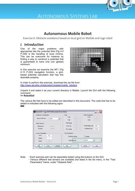
AUTONOMOUS SYSTEMS LABAutonomous Mobile RobotExercise 6: Obstacle avoidance based on local grid on Matlab and Lego robotI. IntroductionOne of the major problems withapproaches like the potential field (Fig 6.5P.258) is the handling of local minima.This can be overcome for instance byfinding a way to construct a potential thatis guaranteed to have only one (global)minimum.In this exercise we examine the NF1 (Fig6.15 P.283) navigation function, a gridbasedpotential calculation that has thisdesirable property.In order to perform this exercise, download the zip file from:http://www.asl.ethz.ch/education/master/mobile_roboticsUnpack it and select it as your current directory in Matlab. Launch the GUI with the followingcommand:>> RobotGUIThe various file that have to be edited are described in this document. The code that has to beadded is indicated with the following signs:###Note:- Each exercise part can be separately tested using the buttons on the GUI.- Various different test terrains are available and listed in the list menu, in the "TestParameters" frame, under "Obstacle field".Autonomous Mobile Robots – Exercise 6 Page 1

Autonomous Mobile Robots – Exercise 2 Page 2II. Wave PropagationThe basic idea of the NF1 is rather simple: Divide the environment of the robot into equallysized grid cells, mark all cells that are occupied by obstacles, and iteratively construct amonotonically increasing potential starting at the cell that contains the goal.In M-File pseudo-code, one possible way to implement the NF1 is:grid = -2 * ones(dimx, dimy); % unvisited cells contain -2for i = 1:n_obstaclesgrid(obstacle(i, 1), obstacle(i, 2)) = -1; % occupied cells contain -1endgrid(goal(1), goal(2)) = 0;% goal cell is global minimumwhile we're not finishedfor all grid(i, j) that are on the wavefrontpropagate wavefront to the 4 direct neighborsby setting their value to grid(i, j) + 1taking care not to:* exceed the grid dimensions* propagate into obstacles* propagate into already visited cellsif any such neighbors were found,then we're not finishedendincrement the wavefrontendExercise 6.1: Implement Wave PropagationComplete the file Calculate_NF1.m (the ### symbol indicates missing code) such that itperforms wavefront propagation. The code for inserting the obstacles is provided.Test your code using the NF1 button of the GUI.You should obtain the following result (with "normal" obstacle):WARNING: Do not push the Run button at this time!

Autonomous Mobile Robots – Exercise 2 Page 3III. Gradient Descent WaveOnce the NF1 has been constructed, the potential can be descended from robot to goal. Thefollowing M-File pseudocode generates the list of grid indices that lead from the robot cell tothe goal cell:% define the neighborhood setneighbor = [+1 +1 0 -1 -1 -1 0 +1;...% row index0 +1 +1 +1 0 -1 -1 -1 ] '; % column index% start the path at the robot positionpath(1, :) = robot_cell;% follow gradient until we're at the goaln = 1;while path(n, :) is not the goalfor all candidate neighbors% HINT: candidate = path(n, :) + neighbor(i, :);check if the candidate is valid,and if it has the smallest value so far,in which case it should become the best candidateendn = n + 1;path(n, :) = best_candidate;endExercise 6.2: Implement Gradient DescentComplete the file Trace_NF1.m (the ### symbol indicates missing code) such that it performsthe gradient descent. The neighborhood is already defined in the parameter nf1 and can beaccessed using the form nf1.neighbor. Converting the resulting path to global coordinates isdone as part of the already existing code. Test your code using the Trace button of the GUI.You should obtain the following result (with "normal" obstacle):WARNING: Do not push the Run button at this time!

Autonomous Mobile Robots – Exercise 2 Page 4IV.Robot Control, ComparisonExercise 6.3: SimulationComplete the function CalculateSpeed.m (the ### symbol indicates missing code) andsimulate the robot trajectory using the Simulate button of the GUI Use the provided functionDirection_NF1.m, which calculates the gradient direction in the global frame of reference forany given point.Additional information can be found in your reference book (p. 83-86).Note that:• The final state does not take into account the orientation; therefore, β can beneglected.• α is a relative angle between the goal and the robot orientation.• ρ is the minimum value between the distance to the goal and the distance needed tocross two cells of the grid. The cells size corresponds to the robot.radius.You should obtain the following result (with "normal" obstacle):WARNING: Do not push the Run button before it actually works!Exercise 6.4: Implementation on Lego-RobotAfter simulating the rover behaviour, test your implementation with a real Lego-Robot usingthe Run button of the GUI. Select the test terrains "lego test 1" or "lego test 2" to test yourimplementation. The test terrain is defined in the file Initialize.m. You can also define yourown map by modifying any of the existing terrains (e.g. "foo") but consider the limited spaceyou have for your experiments.Modify and optimize the control parameters Krho and Kalpha (in the GUI) and identify thecorresponding effects. Do you notice any difference between the simulation and the realtests?Exercise 6.5: Comparison with Potential FieldWhen compared with the potential field method (Fig 6.5 P.258), what advantages anddrawbacks can you identify for the NF1? Are their respective strength and weaknessescomplementary?

Autonomous Mobile Robots – Exercise 2 Page 5V. Annex: Coordinate Transformations and Grid IndicesIn order to be of use for controlling areal robot, the discrete gridrepresentation of the NF1 has to bematched to meaningful coordinatesand vice-versa. The M-Files used inthis exercise perform this task for you.The file Create_Transformer.minitializes a data structure that cansubsequently be used in the functionsFrom_Transformer.mandTo_Transformer.m to transform agiven point either from the globalcoordinate system to a local one, orvice-versa. Once a point has beentransformed from the global frame tothe grid's frame of reference, a simplelinear relation of the form:ix= round(( x + doff) / Δ)can be used to find its correspondingindices.Finding a grid cell's coordinates in the global frame implies inverting that linear relation andthen transforming it to the global frame. The files FLength_NF1.m and FIndex_NF1.mimplement the above mentioned linear equations.Examples of use can be seen in the files Create_NF1.m, Calculate_NF1.m, Trace_NF1.mand Direction_NF1.m.